"Python Programming for Geospatial Data Science." BAKHAT ALI.pdf

2 GEOPYTHON PYTHON PROGRAMMING FOR GEOSPATIAL DATA SCIENCE Introduction to Geospatial Data Science Geospatial Data Science integrates spatial data analysis, Geographic Information Systems (GIS), remote sensing, and advanced data science techniques to interpret and address complex spatial challenges. Its significance spans multiple domains including: Urban Planning: Infrastructure development, zoning Environmental Conservation: Habitat mapping, climate change studies Disaster Management: Risk assessment, emergency response Transportation: Route optimization, traffic analysis Public Health: Disease mapping, resource allocation Primary Data Types: Vector Data: Discrete features such as points (e.g., sensors), lines (e.g., roads), and polygons (e.g., lakes, administrative boundaries) Raster Data: Continuous data including satellite imagery, elevation models, temperature maps, land cover classifications Role of Python Ecosystem: Python offers extensive libraries (GeoPandas, Rasterio, etc.) that enable automation, scalable processing, and efficient analysis of spatial data. Tools like Anaconda and Jupyter Notebooks streamline environment management, fostering interactive, reproducible workflows.

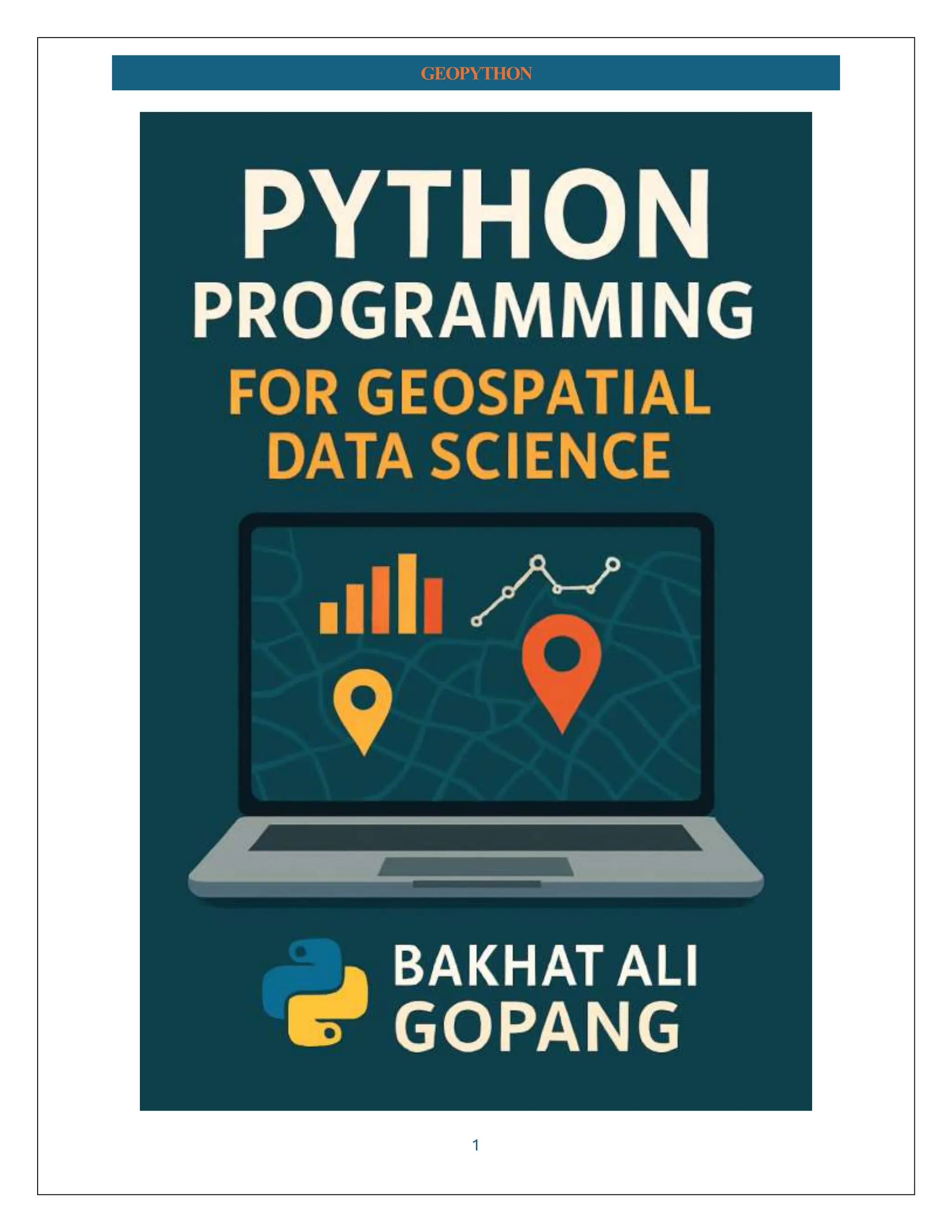
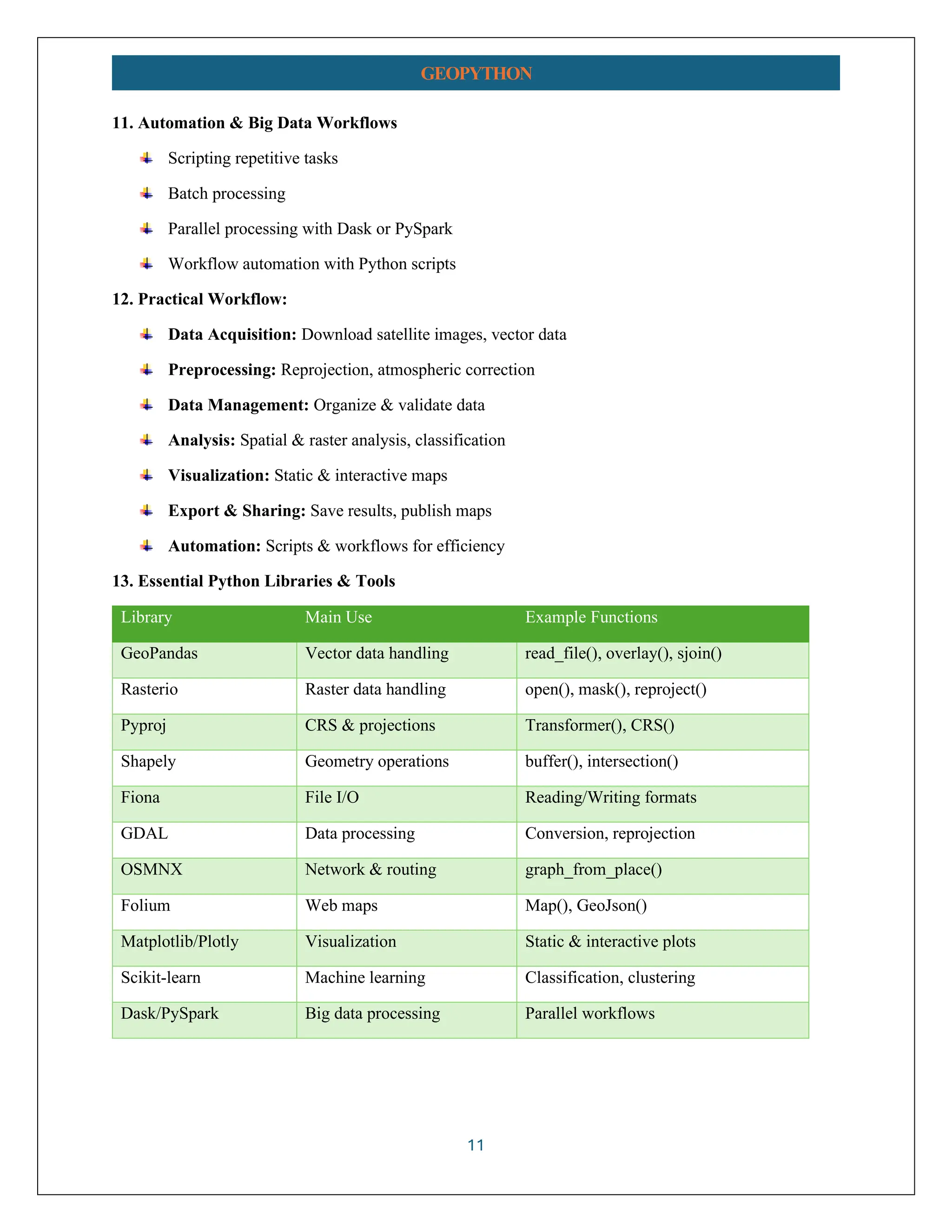
3 GEOPYTHON Lab 1: Setting Up Python for Geospatial Data Step 1: Install Anaconda Step 2: Create and activate a dedicated environment conda create -n geo_env python=3.8 -y conda activate geo_env Step 3: Install essential geospatial libraries conda install geopandas rasterio jupyter -y Step 4: Launch Jupyter Notebook for interactive coding jupyter notebook Start exploring and analyzing geospatial data efficiently with Python! Basic Python for Geospatial Data Science 1. Variables and Data Types • Store data such as coordinates, attributes latitude = 40.7128 longitude = -74.0060 city_name = "New York" population = 8_336_817 2. Lists and Dictionaries • Manage collections of data # List of coordinates coords = [(40.7128, -74.0060), (34.0522, -118.2437)] # Dictionary for attributes city_info = { "name": "New York", "population": 8_336_817, "coordinates": (40.7128, -74.0060) } 3. Functions • Reusable blocks of code

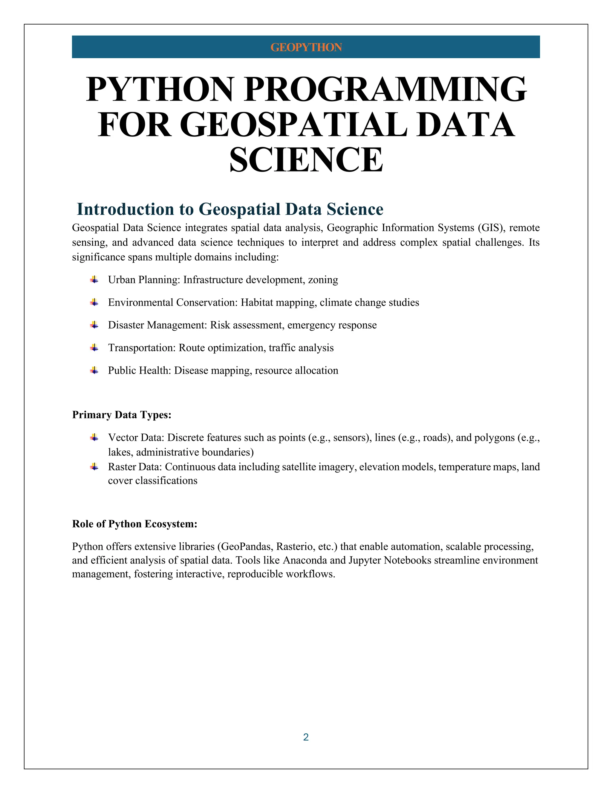
4 GEOPYTHON def get_area(length, width): return length * width area = get_area(10, 5) 4. Conditional Statements • Make decisions if population > 1_000_000: print("Large city") else: print("Small city") 5. Loops • Iterate over data for city in ["NYC", "LA", "Chicago"]:print(city) 6. Importing Libraries • Use specialized tools for geospatial data Runimport geopandas as gpd import rasterio 7. Reading Geospatial Data • Read a shapefile with GeoPandas gdf = gpd.read_file('path_to_shapefile.shp') print(gdf.head()) 8. Plotting Data • Visualize geographic data gdf.plot()

5 GEOPYTHON Python Fundamentals for Geospatial Data Building a strong foundation involves mastering Python syntax, data structures, and control flow. Key points include: Variables & Data Types storing spatial and attribute data Lists & Tuples managing collections of locations or geometries Dictionaries feature attribute storage Conditional Logic (if, elif, else) — decision-making based on data attributes or spatial relations Loops (for, while) batch processing of features or datasets Functions modular code for spatial analysis and data processing Importing Libraries geopandas, shapely, rasterio, folium, matplotlib Reading Geospatial Data shapefiles, GeoJSON, raster data DataFrame Operations filtering, aggregating, and analyzing attribute data Plotting & Visualization static maps, interactive maps with Folium, Matplotlib CRS Management coordinate system transformations and projections Geometric Operations buffering, intersection, union, difference Filtering Data & Spatial Queries selecting features based on location or attributes Raster Data Analysis reading, masking, classification Data Export & Saving shapefiles, GeoJSON, CSV, raster formats Batch Processing & Automation processing multiple files or datasets in loops Error Handling & Debugging :try-except blocks, logging Scripting & Workflow Automation : integrating steps into scripts Interactive Notebooks Jupyter for exploration, visualization, and sharing Web & API Integration fetching data from OpenStreetMap, Mapbox, or other services

6 GEOPYTHON Lab Exercises :2 Exercise 1: Variables & Data Types • Create variables for a city’s latitude, longitude, and population. • Print out a summary statement. Exercise 2: Lists and Tuples • Store multiple city names in a list. • Convert it to a tuple. • Access the second city. Exercise 3: Dictionaries • Create a dictionary with city names as keys and populations as values. • Retrieve and print the population of a specific city. Exercise 4: Conditional Statements • Write a function that checks if a city’s population is over 1 million. Exercise 5: Loops • Loop through a list of cities and print their names. Exercise 6: Functions • Write a function to calculate the distance between two points. Exercise 7: Import Libraries • Import geopandas, shapely.geometry, and matplotlib.pyplot. Exercise 8: Reading Data Files • Load a shapefile of city boundaries using geopandas. Exercise 9: DataFrame Operations • Filter cities with populations over 500,000. Exercise 10: Plotting Data • Plot city boundaries and label each city.

7 GEOPYTHON Exercise 11: CRS Management • Check and change the CRS of a GeoDataFrame. Exercise 12: Geometric Operations • Create a buffer zone around a city point. Exercise 13: Filtering Spatial Data • Select cities within a certain polygon boundary. Exercise 14: Raster Data Handling • Read a raster image (e.g., satellite image) with rasterio. Exercise 15: Export Data • Save filtered cities as a new shapefile. Exercise 16: Batch Processing • Loop through multiple shapefiles in a folder and combine them. Exercise 17: Error Handling • Wrap file reading in try-except to handle missing files. Exercise 18: Automate a Workflow • Create a script that reads data, processes, and exports results. Exercise 19: Jupyter Notebook • Use a notebook to visualize data interactively. Exercise 20: Web API Data Fetching • Use requests to get data from OpenStreetMap API

8 GEOPYTHON Mastering Spatial Data with Python Spatial data manipulation is at the heart of geospatial analysis: GeoPandas: Extends pandas for spatial data, enabling reading of shapefiles, GeoJSON, and performing spatial joins and overlays. Rasterio: Handles raster data reading satellite imagery, performing pixel-wise operations, and exporting processed images. Coordinate Reference Systems (CRS): Ensures datasets align correctly; transformations are performed via Pyproj. Spatial Operations: ❖ Buffer zones around features. ❖ Clipping datasets to specific study areas. ❖ Merging datasets for comprehensive analysis. Understanding coordinate systems and projections is essential for accurate spatial analysis. Master GIS & RS with Python: 1. Fundamental Concepts of GIS & RS GIS (Geographic Information Systems) Spatial data representation (vector & raster) Coordinate Reference Systems (CRS) Spatial relationships & topology Map projections & transformations Spatial analysis (buffer, overlay, proximity) Cartography & visualization RS (Remote Sensing) Satellite & aerial imagery Spectral bands & indices (NDVI, SAVI) Image preprocessing (atmospheric correction, ortho-rectification) Image classification (supervised & unsupervised) Change detection DEM & terrain analysis

9 GEOPYTHON 2. Core Data Types & Formats Data Type Formats Python Libraries Description Vector Shapefile (.shp), GeoJSON, GPKG, KML GeoPandas, Fiona Points, Lines, Polygons Raster GeoTIFF, IMG Rasterio, GDAL Satellite images, DEMs 3. Spatial Data Handling & Management Reading/writing vector & raster data Managing CRS & projections Data cleaning & validation Creating & editing geometries Spatial joins & overlays Data optimization & indexing 4. Coordinate Reference Systems & Transformations Understanding EPSG codes Reproject datasets Transform coordinate systems Ensuring spatial alignment 5. Spatial Data Operations & Analysis Vector Analysis Buffering: Creating zones around features Clipping: Extracting features within boundaries Overlay: Union, intersection, difference Spatial Join: Attribute transfer based on location Dissolve: Merge polygons based on attributes Nearest neighbor & proximity analysis Raster Analysis Clipping & masking Raster calculation: NDVI, slope, aspect Reprojection & resampling Terrain analysis: Hillshade, aspect, slope Change detection

10 GEOPYTHON 6. Remote Sensing Image Processing Image preprocessing (orthorectification, atmospheric correction) Spectral indices calculation (NDVI, NDWI) Image classification: ▪ Supervised (training samples) ▪ Unsupervised (clustering) Accuracy assessment Change detection methods Feature extraction & segmentation 7. Spatial Indexing & Optimization R-tree for fast querying Spatial indexing with Rtree library Handling large datasets efficiently 8. Visualization & Web Mapping Static maps with GeoPandas & Matplotlib Interactive maps with Folium & Plotly Map design principles Publishing maps & dashboards (Streamlit, Dash 9. Advanced GIS & RS Techniques Network analysis (routing, shortest path) 3D Analysis (terrain modeling, line-of-sight) Geostatistics (kriging, interpolation) Terrain analysis & watershed modeling Machine learning for classification & regression 10. Data Storage & Sharing Spatial databases (PostGIS, SpatiaLite) Data formats & standards Metadata management Cloud storage & processing (AWS, Google Earth Engine)

11 GEOPYTHON 11. Automation & Big Data Workflows Scripting repetitive tasks Batch processing Parallel processing with Dask or PySpark Workflow automation with Python scripts 12. Practical Workflow: Data Acquisition: Download satellite images, vector data Preprocessing: Reprojection, atmospheric correction Data Management: Organize & validate data Analysis: Spatial & raster analysis, classification Visualization: Static & interactive maps Export & Sharing: Save results, publish maps Automation: Scripts & workflows for efficiency 13. Essential Python Libraries & Tools Library Main Use Example Functions GeoPandas Vector data handling read_file(), overlay(), sjoin() Rasterio Raster data handling open(), mask(), reproject() Pyproj CRS & projections Transformer(), CRS() Shapely Geometry operations buffer(), intersection() Fiona File I/O Reading/Writing formats GDAL Data processing Conversion, reprojection OSMNX Network & routing graph_from_place() Folium Web maps Map(), GeoJson() Matplotlib/Plotly Visualization Static & interactive plots Scikit-learn Machine learning Classification, clustering Dask/PySpark Big data processing Parallel workflows

12 GEOPYTHON 14.Resources and tools : GeoPandas documentation Rasterio tutorials QGIS and ArcGIS for GIS fundamentals Google Earth Engine for large-scale RS OpenStreetMap & OSMnx for network analysi GIS & Remote Sensing with Python: Labs & Exercises Lab 1: Loading and Visualizing Vector Data Objective: Load a shapefile and visualize it. Tasks: • Load a city boundary shapefile. • Plot the boundary using GeoPandas. import geopandas as gpd import matplotlib.pyplot as plt # Load vector data gdf = gpd.read_file('city_boundary.shp') # Plot gdf.plot() plt.title('City Boundary') plt.show() Lab 2: Coordinate Reference System (CRS) Transformation Objective: Reproject data to a different CRS. Tasks: • Check the current CRS. • Reproject to EPSG:3857 (Web Mercator). • Visualize both original and reprojected data. # Check CRS print(gdf.crs)

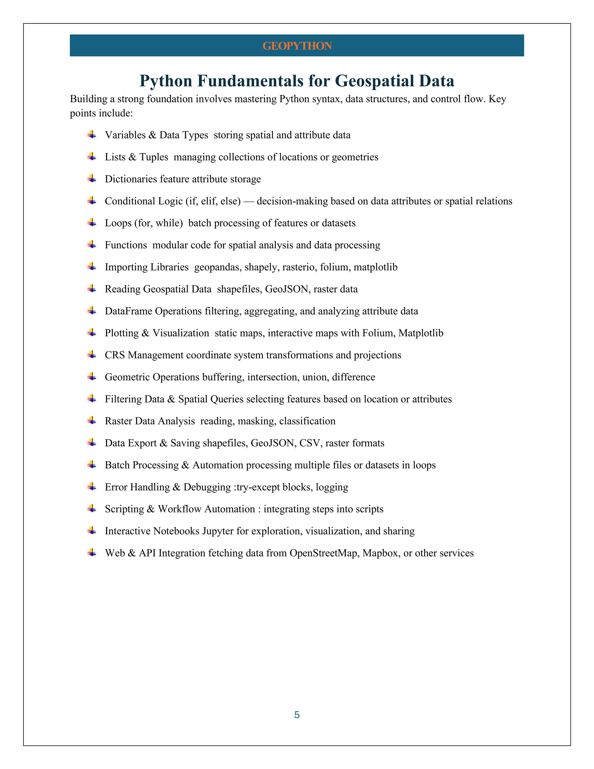
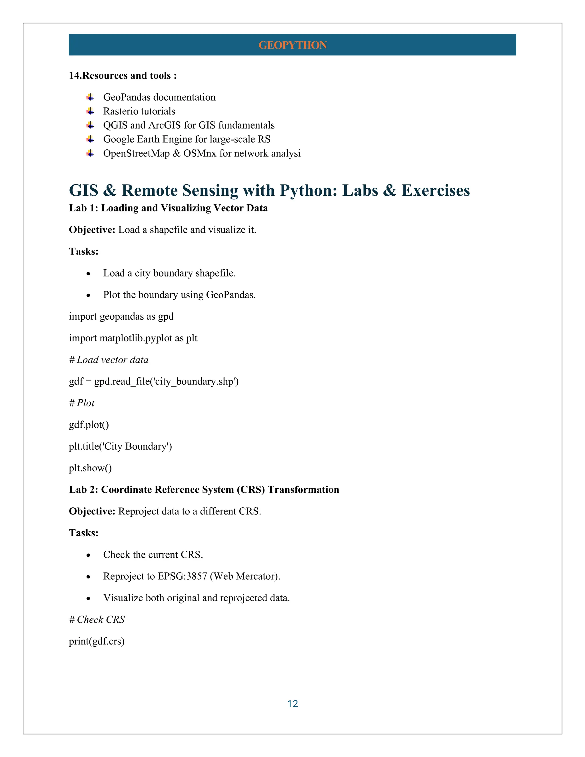
13 GEOPYTHON # Reproject gdf_webmercator = gdf.to_crs(epsg=3857) # Plot original and reprojected fig, axes = plt.subplots(1, 2, figsize=(12, 6)) gdf.plot(ax=axes[0], title='Original CRS') gdf_webmercator.plot(ax=axes[1], title='Reprojected CRS (EPSG:3857)') plt.show() Lab 3: Spatial Clipping Objective: Clip a raster to the boundary of a vector polygon. Tasks: • Load a raster (satellite image). • Clip the raster to the city boundary. import rasterio from rasterio.mask import mask # Load vector boundary boundary = gdf.geometry.unary_union # Load raster with rasterio.open('satellite_image.tif') as src: out_image, out_transform = mask(src, [boundary], crop=True) out_meta = src.meta.copy() # Save clipped raster out_meta.update({"height": out_image.shape[1], "width": out_image.shape[2], "transform": out_transform}) with rasterio.open('clipped_satellite.tif', 'w', **out_meta) as dest: dest.write(out_image)

14 GEOPYTHON Lab 4: Calculating NDVI (Normalized Difference Vegetation Index) Objective: Compute NDVI from multispectral satellite imagery. Tasks: • Load multispectral raster bands. • Calculate NDVI. • Visualize NDVI. import numpy as np import matplotlib.pyplot as plt # Load bands (assuming band 4 = NIR, band 3 = Red) with rasterio.open('satellite_b4.tif') as src: nir = src.read(1).astype('float32') with rasterio.open('satellite_b3.tif') as src: red = src.read(1).astype('float32') # Calculate NDVI ndvi = (nir - red) / (nir + red) ndvi = np.clip(ndvi, -1, 1) # Plot NDVI plt.imshow(ndvi, cmap='RdYlGn') plt.colorbar(label='NDVI') plt.title('NDVI Map') plt.show Lab 5: Point-in-Polygon Analysis Objective: Find which points fall within a given polygon. Tasks: • Load point data (city facilities). • Spatial join with city boundary. • Plot points inside and outside boundary.

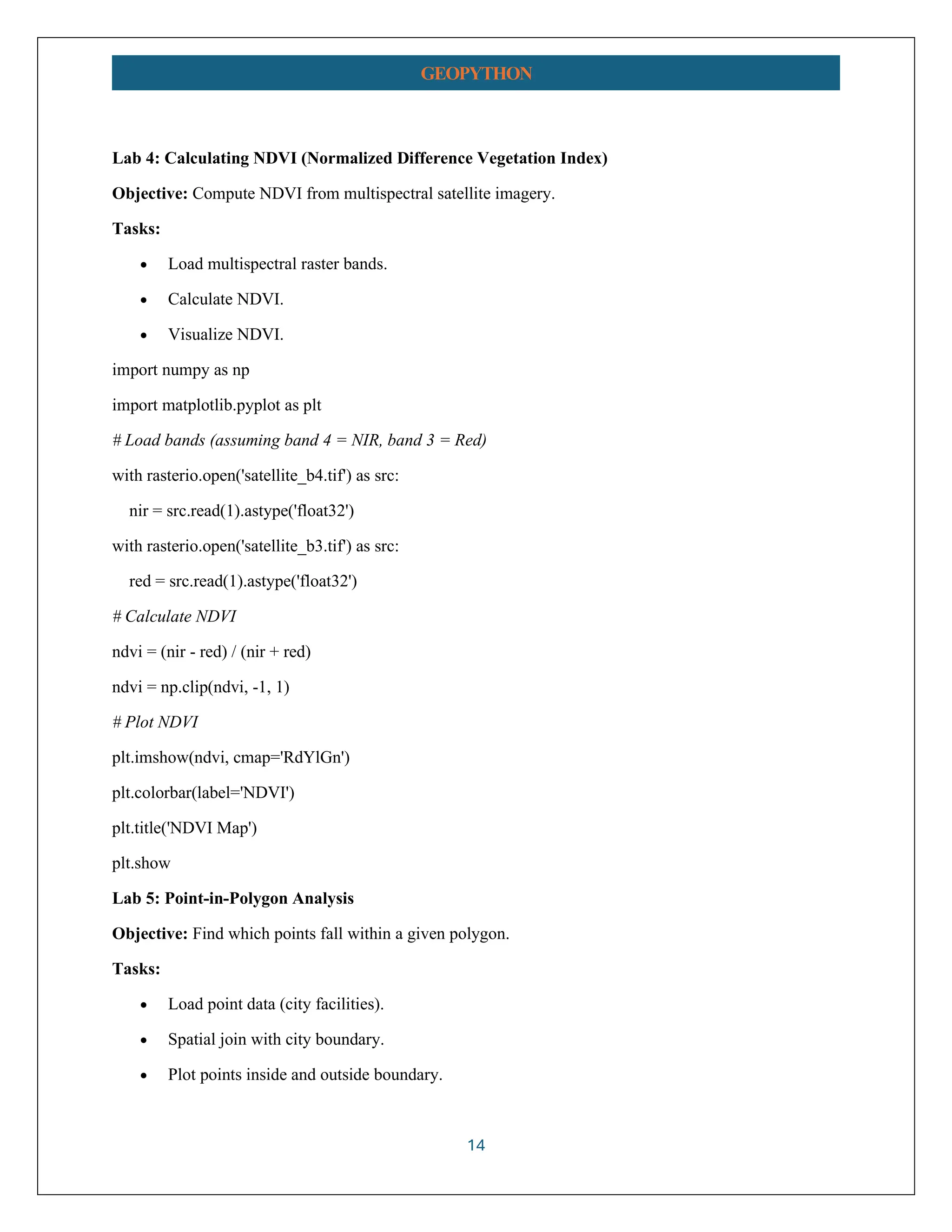
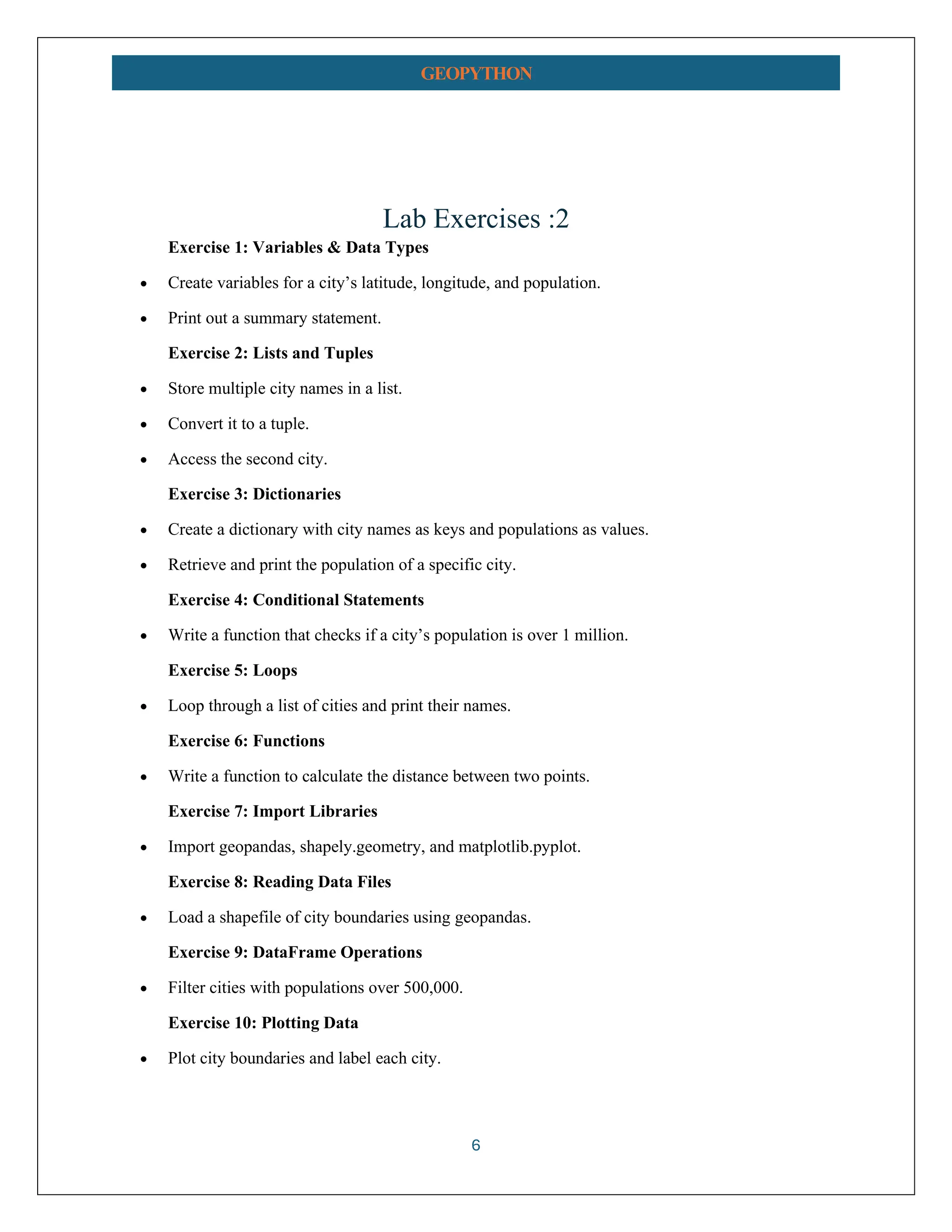
15 GEOPYTHON # Load points points = gpd.read_file('facilities.shp') # Spatial join inside_points = gpd.sjoin(points, gdf, predicate='within') # Plot ax = gdf.plot(color='lightblue') inside_points.plot(ax=ax, color='red', marker='o') plt.title('Facilities within City Boundary') plt.show() Lab 6: Creating an Interactive Map with Folium Objective: Visualize vector data interactively. Tasks: • Load boundary data. • Plot on Folium map. • Add popup info. import folium # Convert GeoDataFrame to GeoJSON geojson_data = gdf.to_json() # Initialize map m = folium.Map(location=[gdf.geometry.centroid.y.mean(), gdf.geometry.centroid.x.mean()], zoom_start=12) # Add GeoJSON layer folium.GeoJson(geojson_data, name='City Boundary').add_to(m) # Save map m.save('city_boundary_map.html')

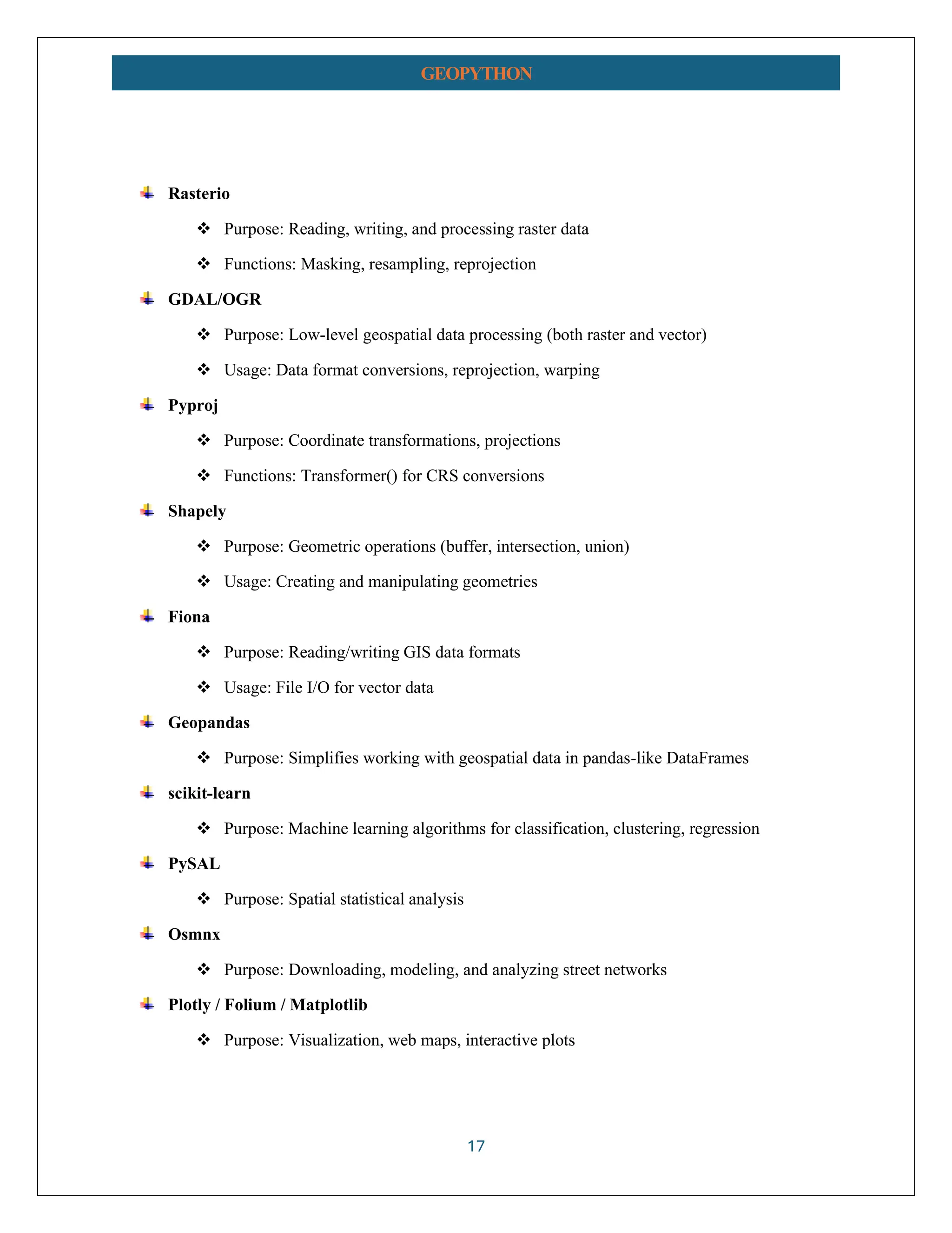
16 GEOPYTHON Lab 7: Network Routing with OSMnx Objective: Find shortest path between two points. Tasks: • Download road network. • Calculate shortest route. import osmnx as ox # Get graph G = ox.graph_from_place('City, Country', network_type='drive') # Find nearest nodes to start and end points orig_point = (latitude1, longitude1) dest_point = (latitude2, longitude2) orig_node = ox.nearest_nodes(G, orig_point[1], orig_point[0]) dest_node = ox.nearest_nodes(G, dest_point[1], dest_point[0]) # Calculate shortest path route = ox.shortest_path(G, orig_node, dest_node, weight='length') # Plot route fig, ax = ox.plot_graph_route(G, route) Spatial Analysis & Modeling Essential Libraries, Software, and Platforms for Geospatial Analysis 1. Python Libraries for Geospatial Analysis Core Geospatial Libraries GeoPandas ❖ Purpose: Handling vector data (shapefiles, GeoJSON) ❖ Functions: Reading, writing, spatial joins, overlays ❖ Example: gpd.read_file()

17 GEOPYTHON Rasterio ❖ Purpose: Reading, writing, and processing raster data ❖ Functions: Masking, resampling, reprojection GDAL/OGR ❖ Purpose: Low-level geospatial data processing (both raster and vector) ❖ Usage: Data format conversions, reprojection, warping Pyproj ❖ Purpose: Coordinate transformations, projections ❖ Functions: Transformer() for CRS conversions Shapely ❖ Purpose: Geometric operations (buffer, intersection, union) ❖ Usage: Creating and manipulating geometries Fiona ❖ Purpose: Reading/writing GIS data formats ❖ Usage: File I/O for vector data Geopandas ❖ Purpose: Simplifies working with geospatial data in pandas-like DataFrames scikit-learn ❖ Purpose: Machine learning algorithms for classification, clustering, regression PySAL ❖ Purpose: Spatial statistical analysis Osmnx ❖ Purpose: Downloading, modeling, and analyzing street networks Plotly / Folium / Matplotlib ❖ Purpose: Visualization, web maps, interactive plots

18 GEOPYTHON Remote Sensing & Image Processing EarthPy (by Earth Lab) ❖ Purpose: Raster processing, visualization Sentinelhub-py ❖ Purpose: Access Sentinel satellite data Google Earth Engine API (ee) ❖ Purpose: Access GEE data, perform large-scale analysis 2. Desktop GIS Software ArcGIS & ArcGIS Pro ArcGIS Desktop (ArcMap) ❖ Commercial GIS software by Esri ❖ Features: Advanced spatial analysis, cartography, data management ArcGIS Pro ❖ Modern GIS desktop application by Esri ❖ Supports Python scripting (ArcPy), 3D analysis, web GIS integration QGIS Open-source GIS software ❖ Features: Vector & raster editing, plugins, spatial analysis ❖ Python integration: PyQGIS API for scripting and automation GRASS GIS ❖ Open-source GIS for raster, vector, geostatistics

19 GEOPYTHON 3. Cloud Platforms & Web-Based Tools Google Earth Engine (GEE) Platform: Cloud-based geospatial analysis platform Languages: JavaScript API, Python API (earthengine-api) Features: Access to petabytes of satellite imagery, large-scale analysis, time-series Sentinel Hub Platform: Cloud-based satellite data access and processing AWS & Azure Use: Hosting large geospatial datasets, running geospatial analysis workflows Category Tools / Libraries Purpose / Use Cases Python Libraries GeoPandas, Rasterio, GDAL, Pyproj, Shapely, Fiona, scikit-learn, Osmnx Data handling, processing, spatial analysis, classification Desktop GIS ArcGIS Pro, ArcMap, QGIS, GRASS GIS Data editing, visualization, analysis Cloud Platforms Google Earth Engine, Sentinel Hub, AWS, Azure Large-scale data access, processing, modeling Spatial analysis techniques include: Buffering: Creating zones around features for proximity analysis. Clipping & Merging: Extracting specific areas or combining datasets. Spatial Joins: Merging attribute data based on spatial relationships. Terrain Analysis: Deriving slope, aspect, and hillshade from DEMs. Hotspot Detection: Identifying clusters of high/low values using spatial statistics

20 GEOPYTHON These tools facilitate environmental modeling, urban planning, and resource management. Google Earth Engine (GEE) with Python GEE provides access to petabytes of satellite imagery and geospatial datasets: Setup: Authenticate and initialize using earthengine-api. Dataset Access: Use GEE’s vast catalog for land cover, climate, and environmental data. Processing: Perform large-scale analyses like deforestation detection or urban growth. Visualization: Use geemap for interactive mapping within Python. Export: Save processed data locally or to cloud storage. GEE accelerates large-scale environmental assessments with minimal local processing. Machine Learning & Data Science in Geospatial Context ML techniques enhance predictive modeling: Data Preparation: Feature extraction, normalization, and splitting datasets. Classification Algorithms: Random Forests, SVMs, and deep learning models classify land cover, detect features. Clustering: K-Means, DBSCAN segment spatial data into meaningful groups. Anomaly Detection: Identify unusual patterns or outliers. Model Validation: Use accuracy metrics, confusion matrices, cross-validation for robust results. Integration of ML with spatial data unlocks insights in urban growth, environmental change, and resource allocation. Time Series & Change Detection Temporal analysis involves: Multi-temporal Data: Analyzing satellite images over time to monitor land cover changes. Change Detection Methods: Image differencing, post-classification comparison, spectral indices. Trend Analysis: Apply statistical models (e.g., ARIMA) to forecast future trends. Visualization: Animations, time-lapse maps, and interactive dashboards illustrate changes over

21 GEOPYTHON Geospatial Data Science Projects: 1. Urban Growth Monitoring Objective: Analyze and visualize urban expansion over time using satellite imagery and vector data. Data Sources: Landsat or Sentinel satellite images, city boundary shapefiles. Tools: Rasterio, GeoPandas, NDVI calculation, time-series analysis. Steps: ❖ Download multi-temporal satellite images. ❖ Preprocess images (cloud masking, atmospheric correction). ❖ Calculate NDVI to identify vegetation loss. ❖ Detect urban expansion by thresholding built-up areas. ❖ Visualize change over time with interactive maps or animations. 2. Flood Risk Assessment Objective: Identify flood-prone areas based on DEMs, rainfall data, and land use. Data Sources: Digital Elevation Models (DEMs), rainfall datasets, land cover maps. Tools: Rasterio, GeoPandas, PySAL. Steps: ❖ Reproject datasets to a common CRS. ❖ Derive slope and flow accumulation. ❖ Overlay land use data to identify vulnerable zones. ❖ Use spatial analysis to delineate flood risk zones. ❖ Generate maps highlighting high-risk areas.

22 GEOPYTHON 3. Public Health & Disease Mapping Objective: Map disease incidence and identify hotspots. Data Sources: Disease case data with location info, demographic data, health facilities. Tools: GeoPandas, Folium, scikit-learn (for clustering), PySAL. Steps: ❖ Load and visualize disease case points. ❖ Perform spatial clustering (e.g., K-Means, DBSCAN). ❖ Create heatmaps of disease density. ❖ Overlay with population density to identify vulnerable zones. ❖ Generate an interactive web map for stakeholders. 4. Route Optimization for Emergency Response Objective: Find the shortest and fastest routes for emergency vehicles. Data Sources: Road network data from OpenStreetMap. Tools: OSMnx, NetworkX, Folium. Steps: ❖ Download road network graph for a city. ❖ Map start and end points (e.g., hospital to incident site). ❖ Calculate shortest path or fastest route considering traffic data. ❖ Visualize routes interactively. ❖ Automate routing for multiple scenarios.

23 GEOPYTHON 5. Land Cover Classification Using Remote Sensing Objective: Classify land cover types from satellite imagery. Data Sources: Multispectral satellite images. Tools: Rasterio, scikit-learn, GDAL. Steps: ❖ Preprocess imagery (stack bands, normalize). ❖ Extract sample pixels for each class (training data). ❖ Train a classifier (Random Forest, SVM). ❖ Classify the entire image. ❖ Validate with ground truth data. ❖ Visualize classification results. 6. Environmental Impact Assessment Objective: Assess deforestation or habitat loss over a region. Data Sources: Historical land cover maps, satellite images. Tools: GeoPandas, Rasterio, change detection algorithms. Steps: ❖ Load multi-temporal land cover maps. ❖ Overlay and compare to detect changes. ❖ Quantify loss or gain of forested areas. ❖ Map hotspots of environmental change. ❖ Generate reports and visualizations.

24 GEOPYTHON 7. Smart City Infrastructure Planning Objective: Optimize locations for new facilities (e.g., parks, hospitals). Data Sources: City demographic data, existing infrastructure, land use. Tools: GeoPandas, Folium, spatial analysis. Steps: ❖ Map existing facilities. ❖ Identify underserved areas. ❖ Use proximity analysis to suggest optimal locations. ❖ Visualize proposals on interactive maps. ❖ Incorporate demographic data to prioritize. Water Climate Disaster : 1. Flood Risk Mapping and Assessment Objective: Identify flood-prone areas based on elevation, rainfall, and land use. Data Needed: DEM (Digital Elevation Model), rainfall data, land use maps. Tools: Rasterio, GeoPandas, Matplotlib, Folium. Approach: ❖ Delineate flood plains using DEM (areas below a certain elevation). ❖ Overlay rainfall data to identify recent flood risks. ❖ Visualize flood zones interactively or statically.

25 GEOPYTHON 2. Drought Severity Monitoring Objective: Map and analyze drought conditions over time. Data Needed: Precipitation time series, drought indices (e.g., SPI, Palmer Drought Severity Index). Tools: Pandas, Rasterio, Folium, Matplotlib. Approach: ❖ Calculate anomalies in rainfall. ❖ Map drought severity spatially. ❖ Track drought progression over months/years. 3. Water Scarcity Hotspot Identification Objective: Find regions facing water shortages. Data Needed: Water availability data, population density, land use. Tools: GeoPandas, Rasterio, Folium. Approach: ❖ Overlay water demand and supply data. ❖ Identify hotspots where demand exceeds supply. ❖ Visualize vulnerable regions. 4. Climate Change Impact on Water Bodies Objective: Analyze changes in lakes, rivers, or reservoirs over time. Data Needed: Satellite images over multiple years. Tools: Rasterio, scikit-learn, OpenCV. Approach: ❖ Classify water bodies location and extent. ❖ Quantify changes. ❖ Visualize trends.

26 GEOPYTHON 5. Early Warning System for Flooding Objective: Develop a system that predicts flood risk based on weather forecasts. Data Needed: Real-time weather data, historical flood records. Tools: Requests, Pandas, Folium. Approach: ❖ Use weather API data. ❖ Apply thresholds to trigger alerts. ❖ Display warnings on maps. Python programming for Geospatial Data Science Aspect Key Points Data Types Vector (shapefiles), Raster (satellite images) Main Libraries GeoPandas, Rasterio, Shapely, Fiona, Pyproj, scikit-learn Key Tasks Data reading, CRS handling, spatial ops, visualization Visualization Matplotlib, Folium, Plotly Remote Sensing NDVI, classification, change detection Analysis Techniques Buffer, clip, overlay, spatial join, raster analysis Automation Batch processing, scripting workflows APIs & Data Sources OpenStreetMap, Google Earth Engine, APIs Applications Urban planning, disaster risk, environmental monitoring Good luck

"Python Programming for Geospatial Data Science." BAKHAT ALI.pdf

More Related Content

Similar to "Python Programming for Geospatial Data Science." BAKHAT ALI.pdf

More from institute of Geoinformatics and Earth Observation at PMAS ARID Agriculture University of Rawalpindi

Recently uploaded

"Python Programming for Geospatial Data Science." BAKHAT ALI.pdf