Download to read offline
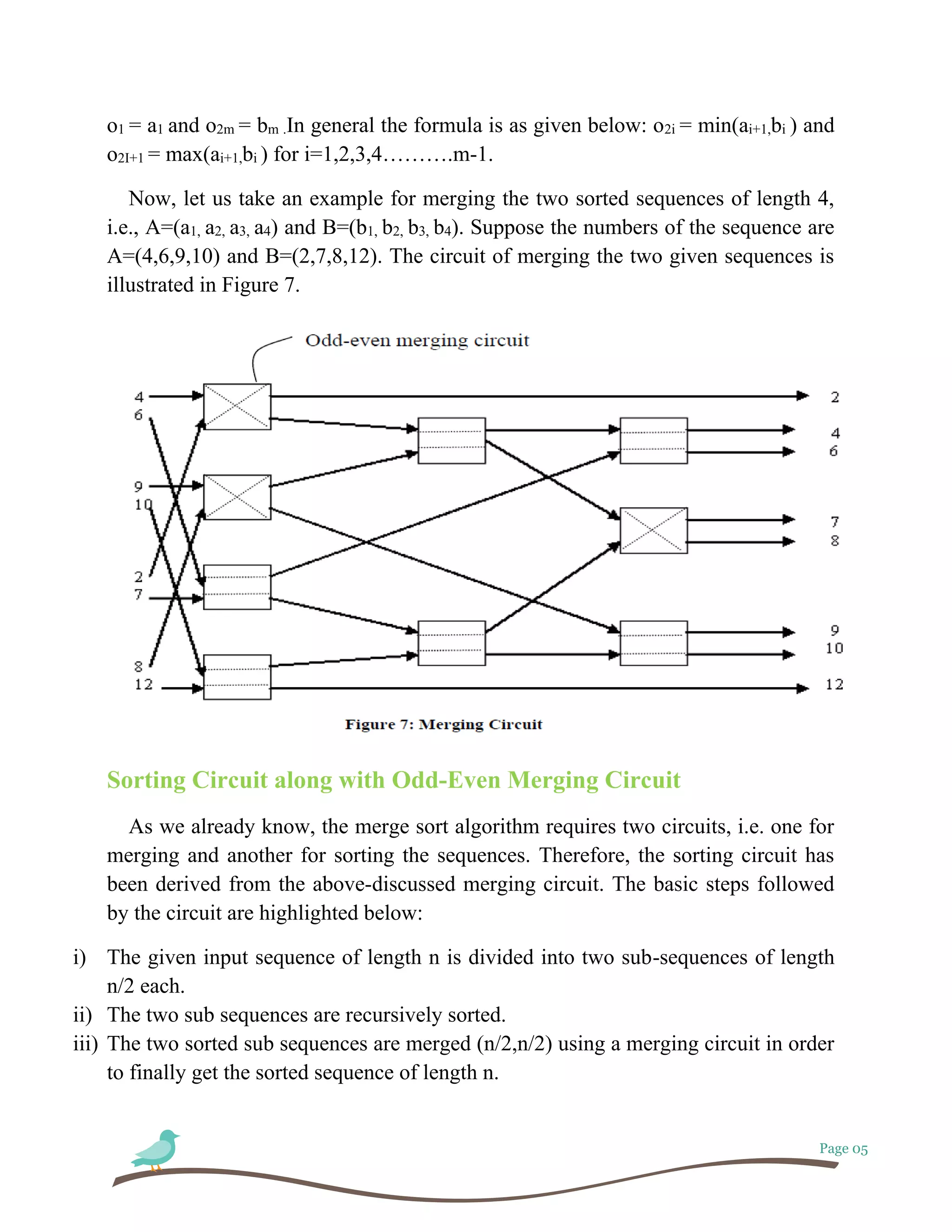
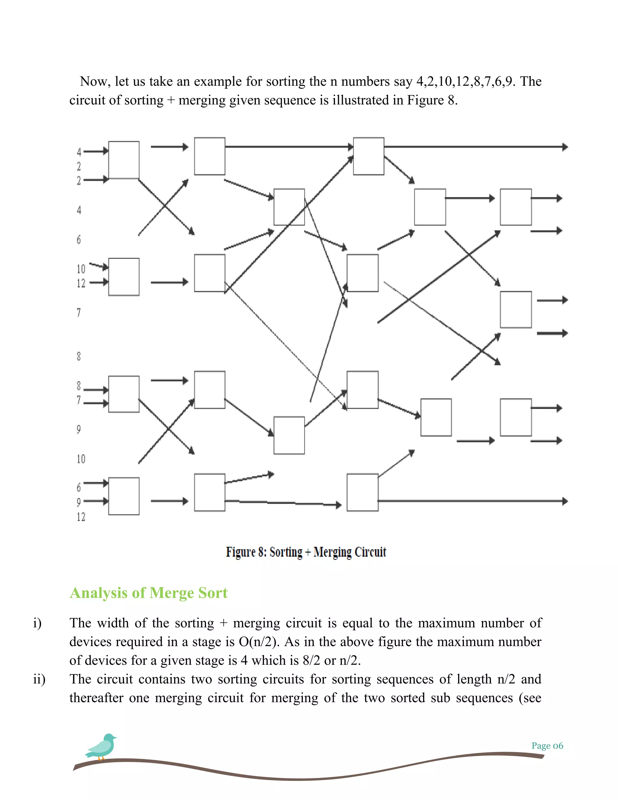

This document discusses algorithms and parallel processing. It begins by defining algorithms and different types of algorithms like sequential and parallel algorithms. It then discusses analyzing parallel algorithms based on time complexity, number of processors required, and overall cost. Specific examples of parallel algorithms discussed include merge sort and parallel image processing. Fault tolerance in parallel systems is also covered, including load distribution, parallel region growing for image segmentation, and the process of system recovery from faults.