Download as PDF, PPTX
![Computing the power iterations using Spark is computed using a treeAggregate operation over the RDD [src: https://databricks.com/blog/2014/09/22/spark-1-1-mllib-performance-improvements.html]!](https://image.slidesharecdn.com/024michaelmahoney-170619124449/75/Matrix-Factorizations-at-Scale-a-Comparison-of-Scientific-Data-Analytics-on-Spark-and-MPI-Using-Three-Case-Studies-with-Michael-Mahoney-25-2048.jpg)
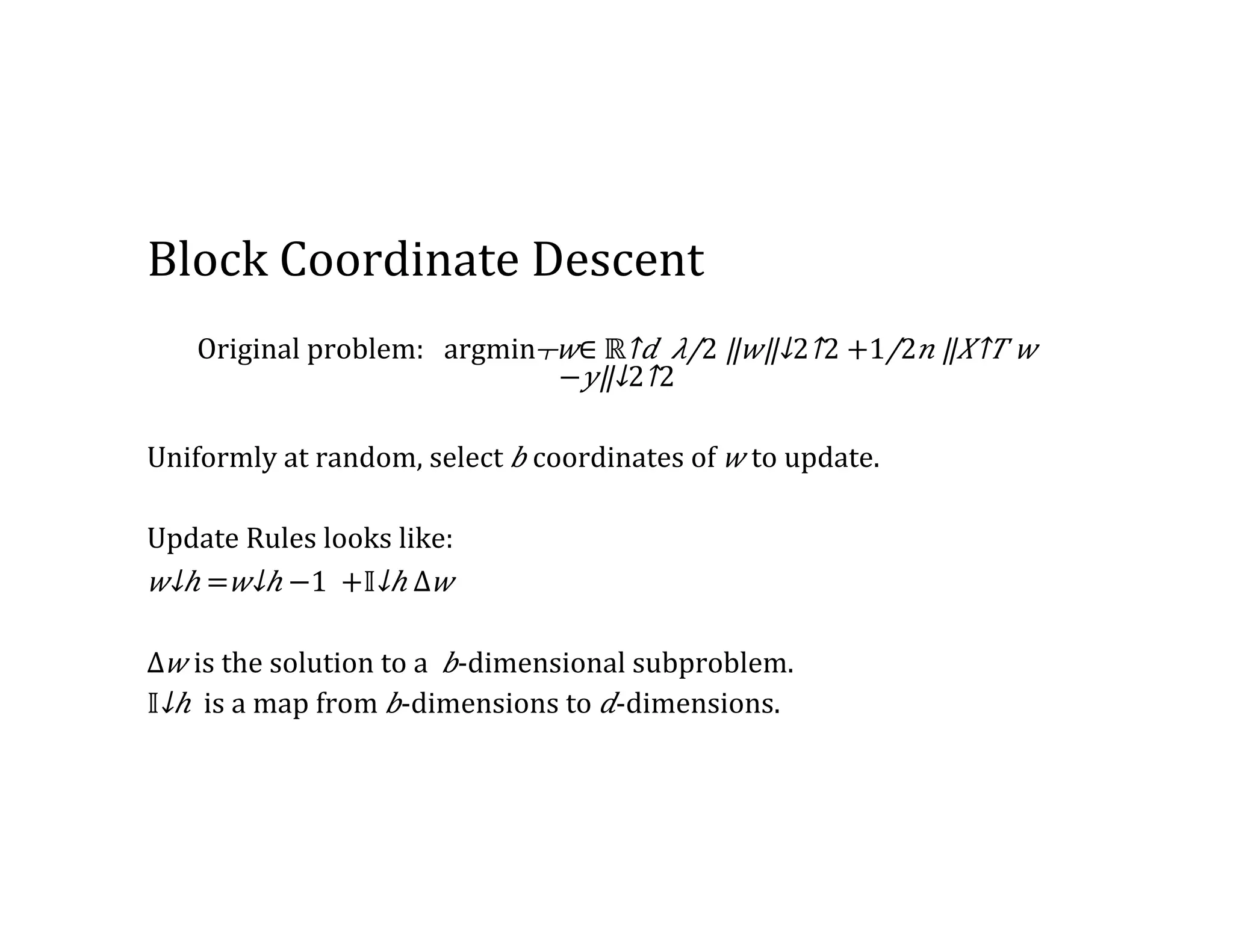
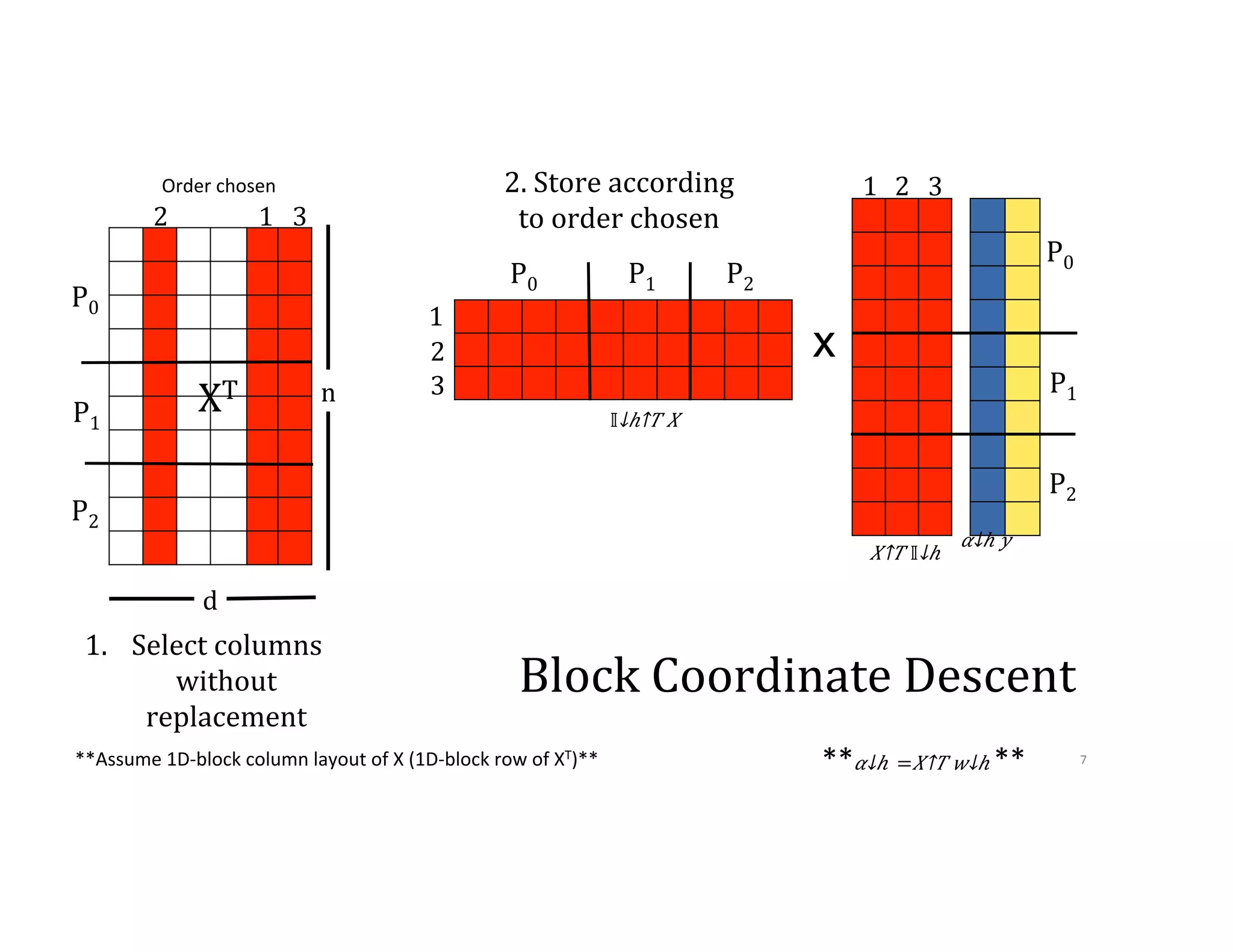
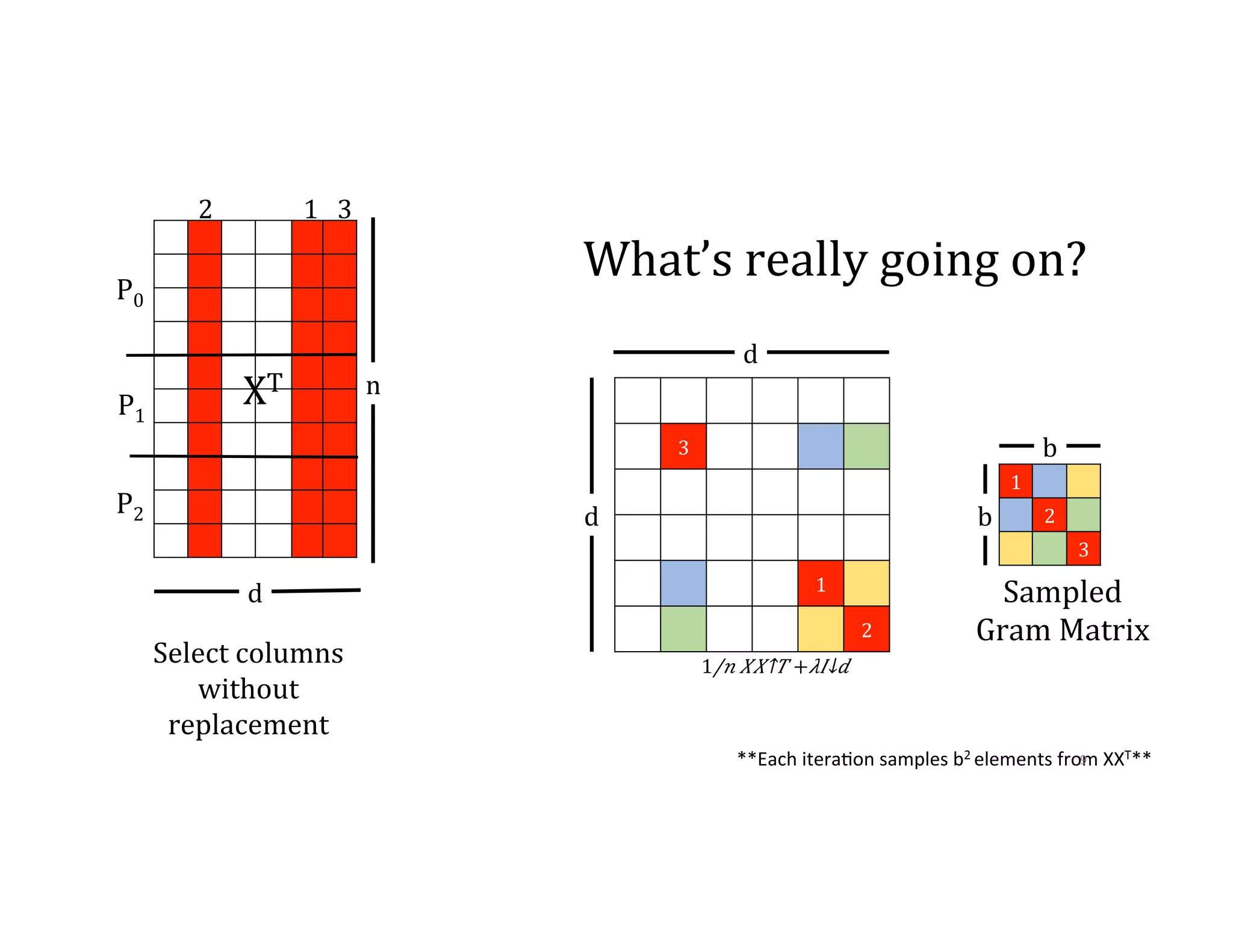
![Communication Avoiding-‐BCD 2 1 3 1 3 2 1. Select columns without replacement 2. Store according to order chosen P0 P1 P2 P0 P1 P2 XT 1,6 3 2,4 n d P0 P1 P2 x 𝛼↓ℎ 𝑦 𝑋↑𝑇 [𝕀↓𝑠𝑘+1 𝕀↓𝑠𝑘+2 ] [█■ 𝕀↓𝑠𝑘+1↑𝑇 𝕀↓𝑠𝑘 +2↑𝑇 ]𝑋 5 4 5 6 4 5 6 10](https://image.slidesharecdn.com/024michaelmahoney-170619124449/75/Matrix-Factorizations-at-Scale-a-Comparison-of-Scientific-Data-Analytics-on-Spark-and-MPI-Using-Three-Case-Studies-with-Michael-Mahoney-59-2048.jpg)
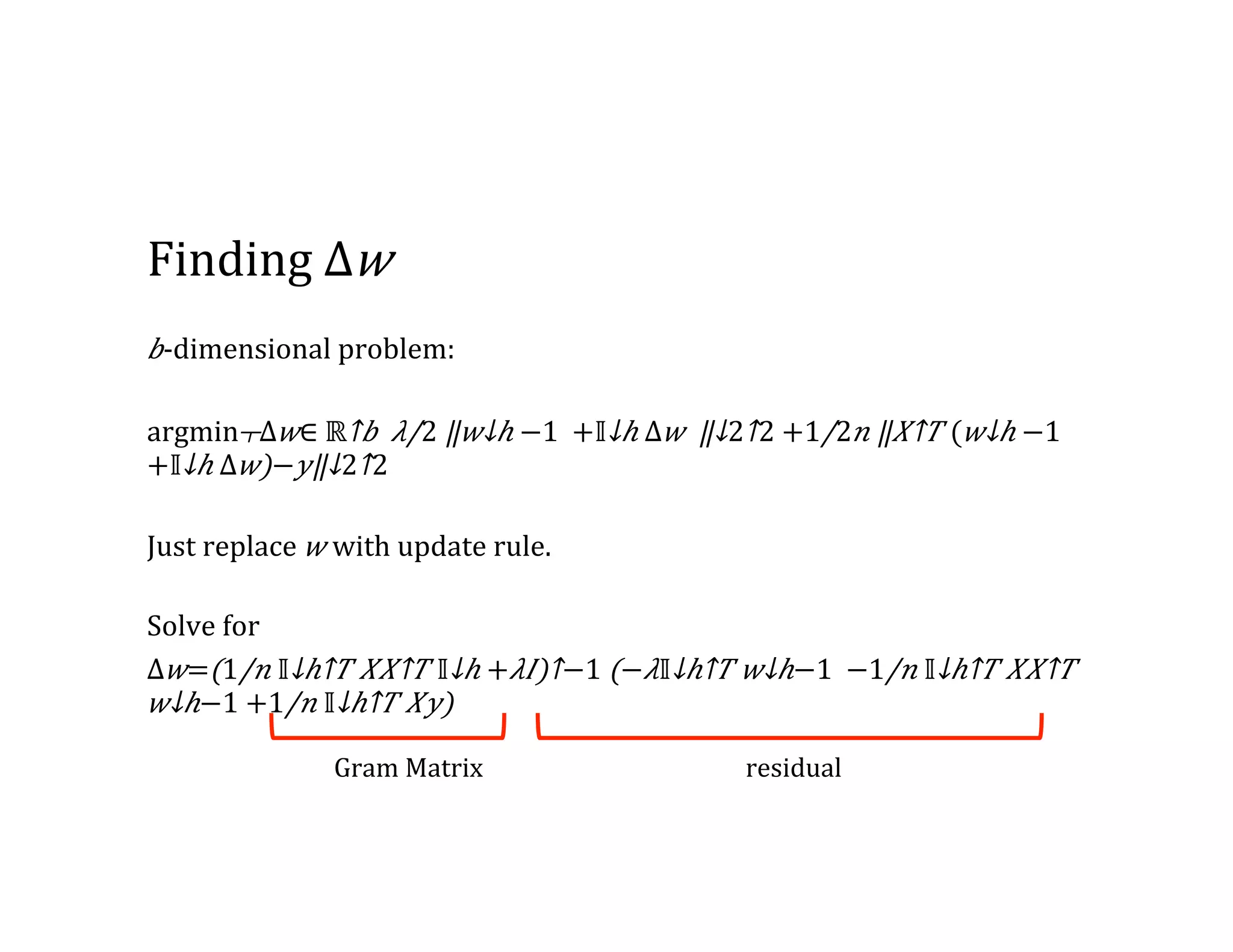
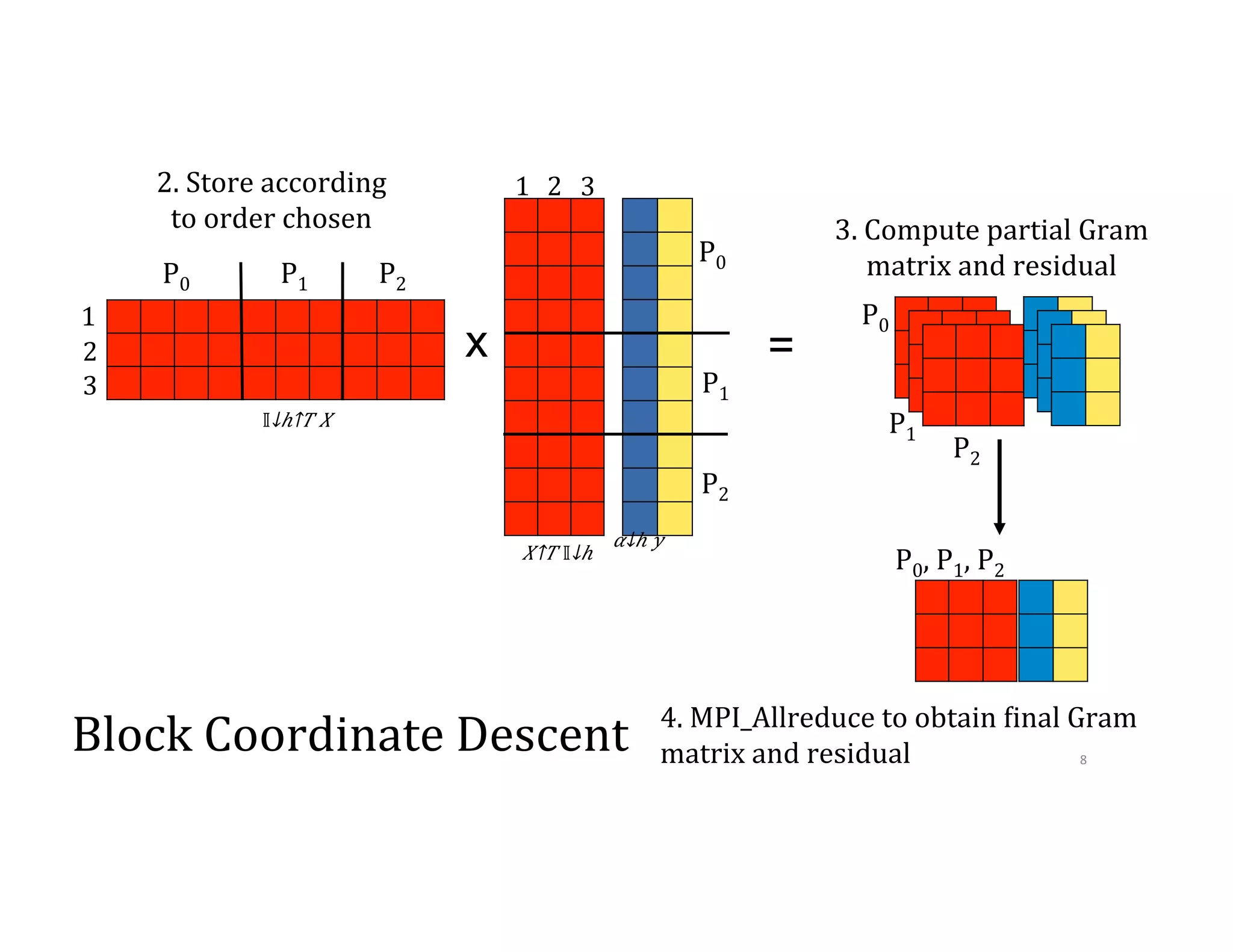
![2 1 3 1 3 2 = 3. Store according to order chosen 4. Compute partial Gram matrix and residual 4. MPI_Allreduce to obtain 9inal Gram matrix and residual P0 P1 P2 P0 P1 P2 P0 P1 P2 P0, P1, P2 x 𝛼↓ℎ 𝑦 𝑋↑𝑇 [𝕀↓𝑠𝑘+1 𝕀↓𝑠𝑘+2 ] [█■ 𝕀↓𝑠𝑘+1↑𝑇 𝕀↓𝑠𝑘 +2↑𝑇 ]𝑋 4 5 6 4 5 6 11](https://image.slidesharecdn.com/024michaelmahoney-170619124449/75/Matrix-Factorizations-at-Scale-a-Comparison-of-Scientific-Data-Analytics-on-Spark-and-MPI-Using-Three-Case-Studies-with-Michael-Mahoney-60-2048.jpg)
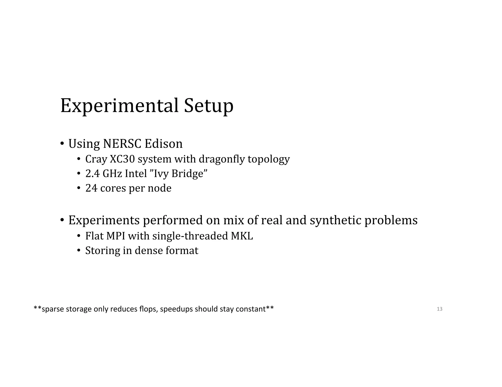
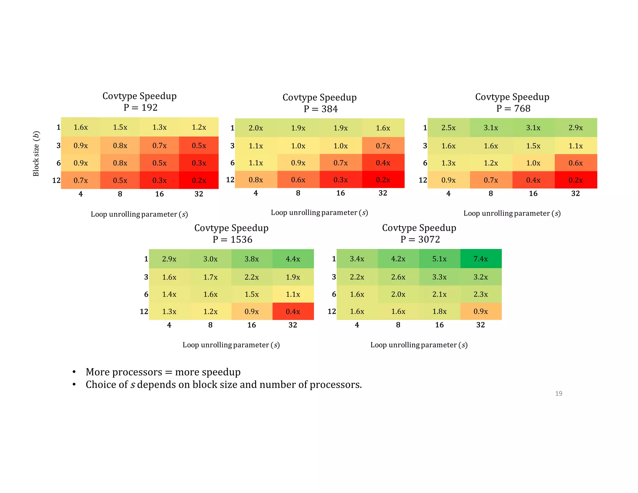

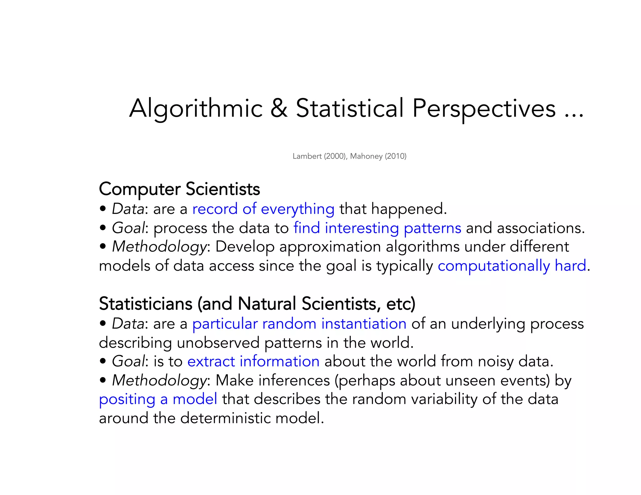
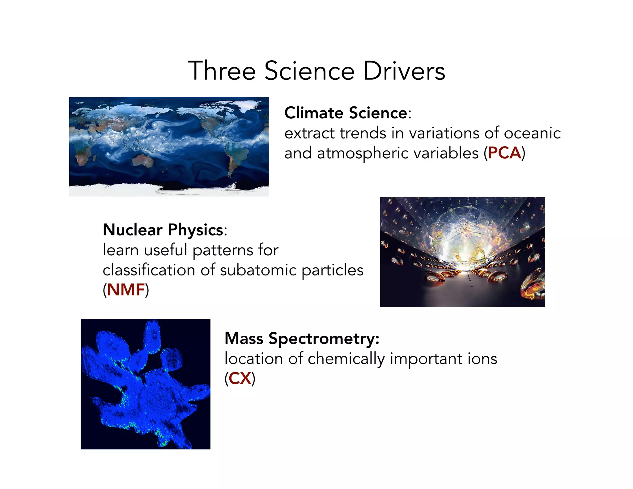
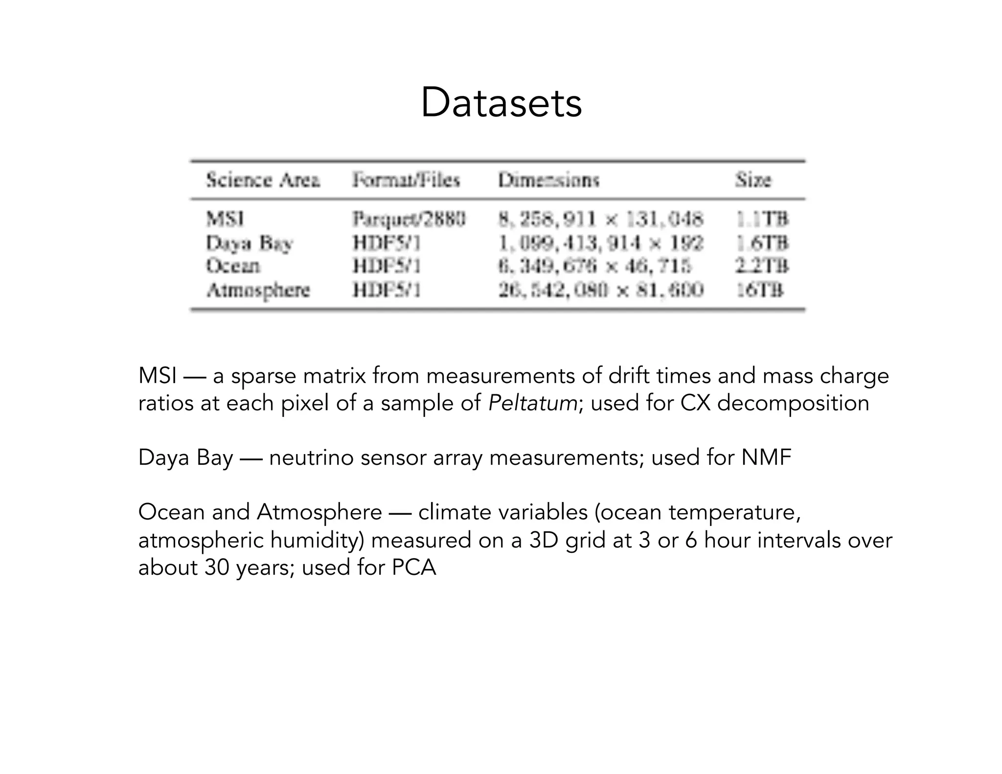
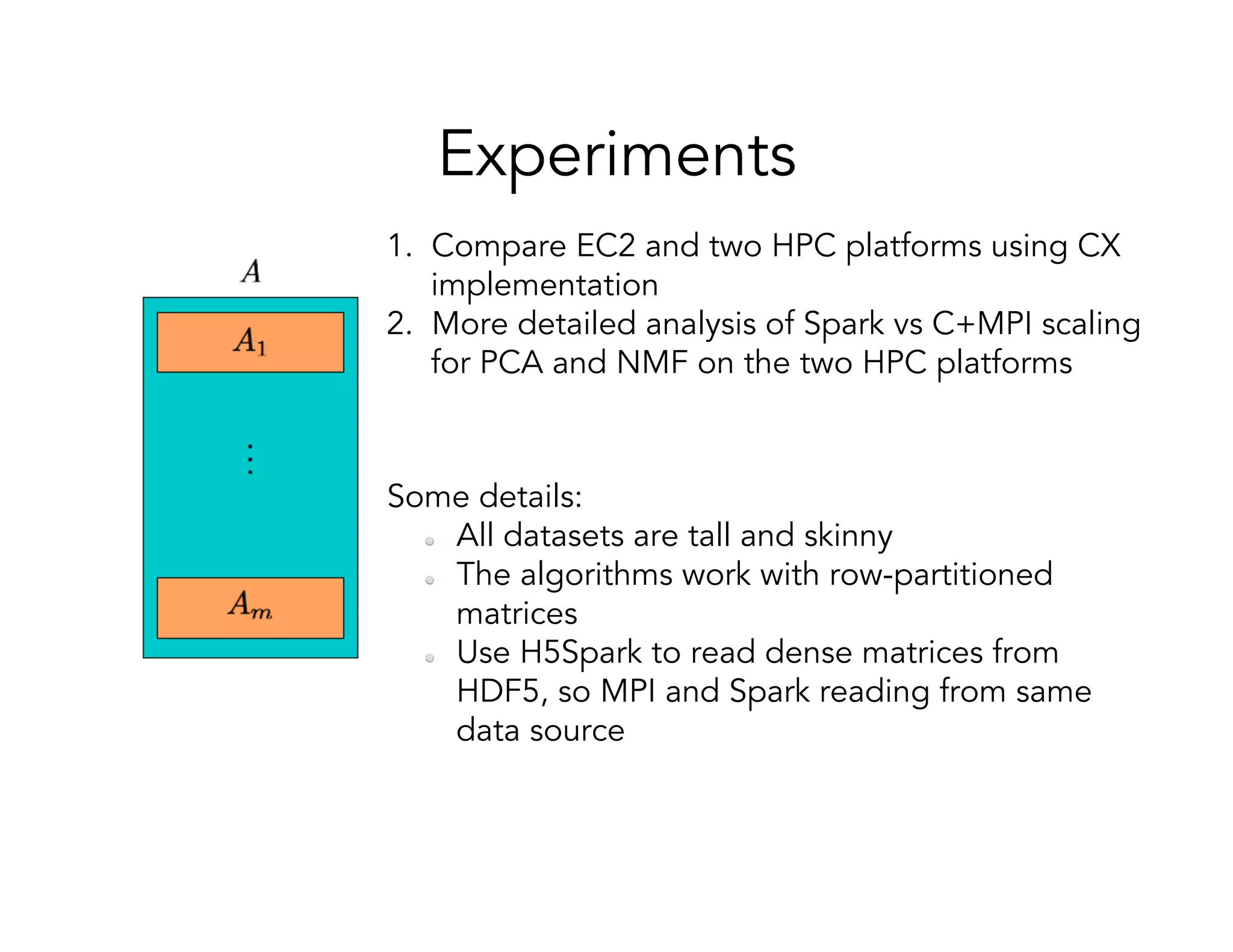
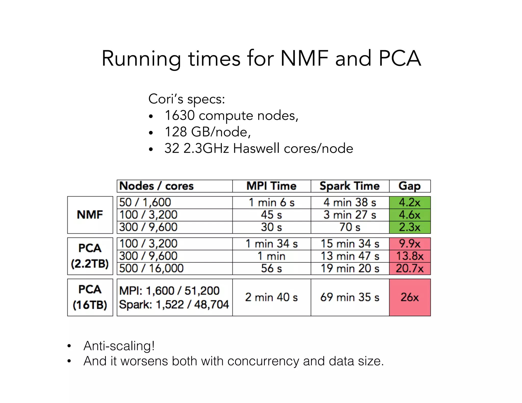
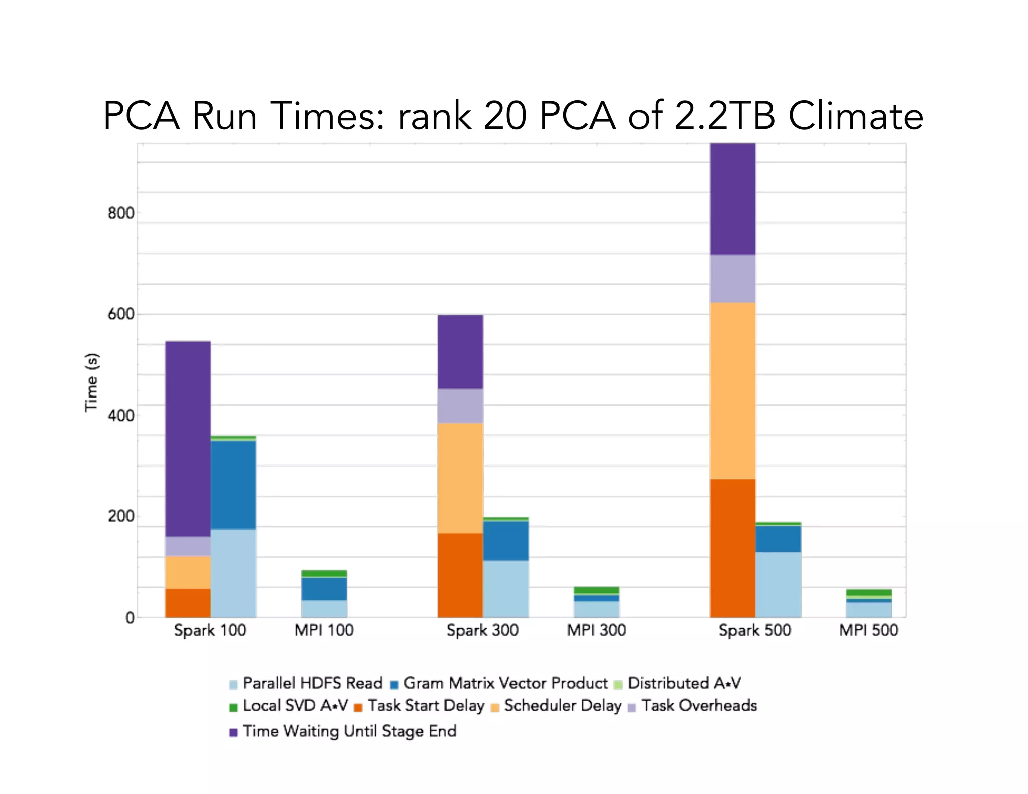
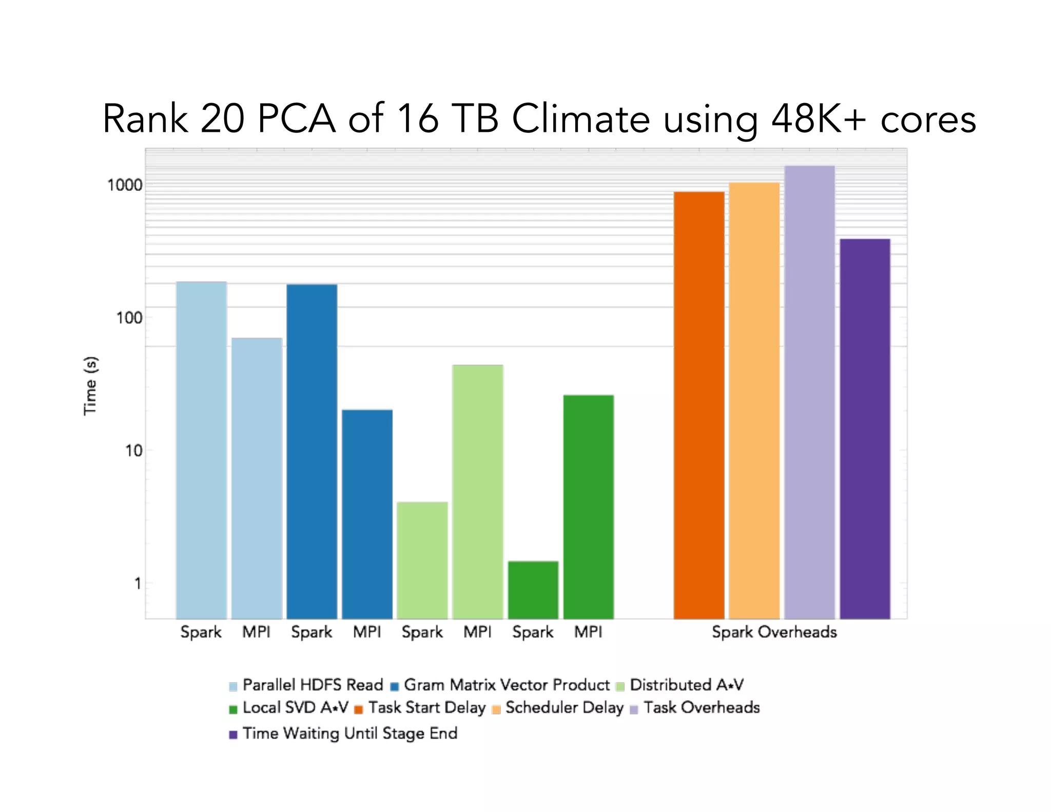
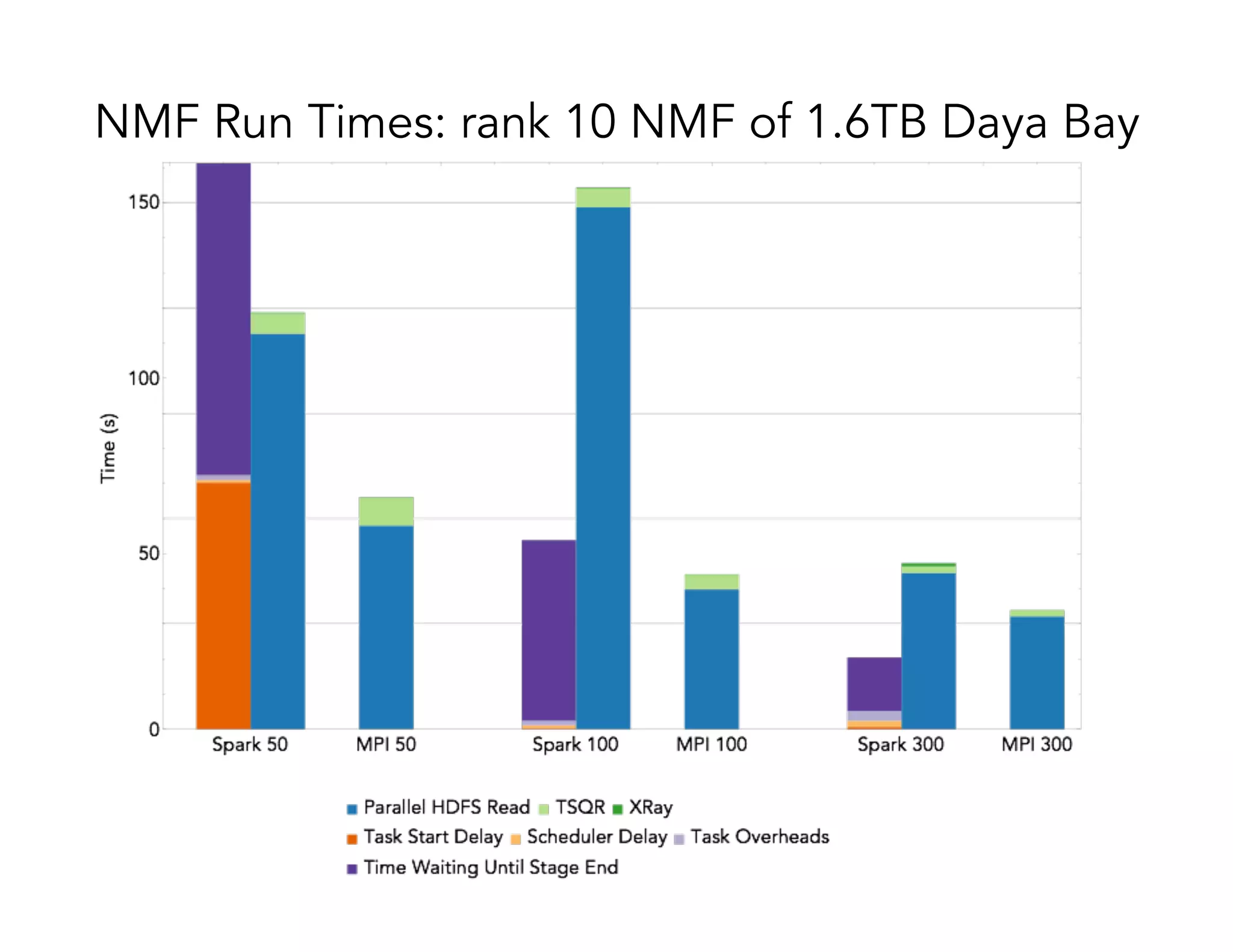
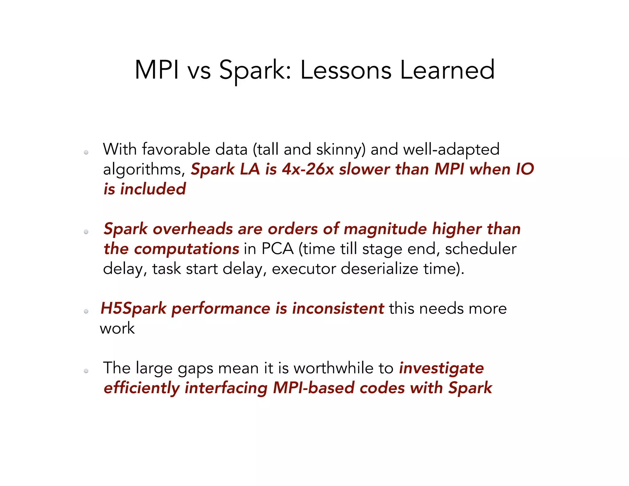
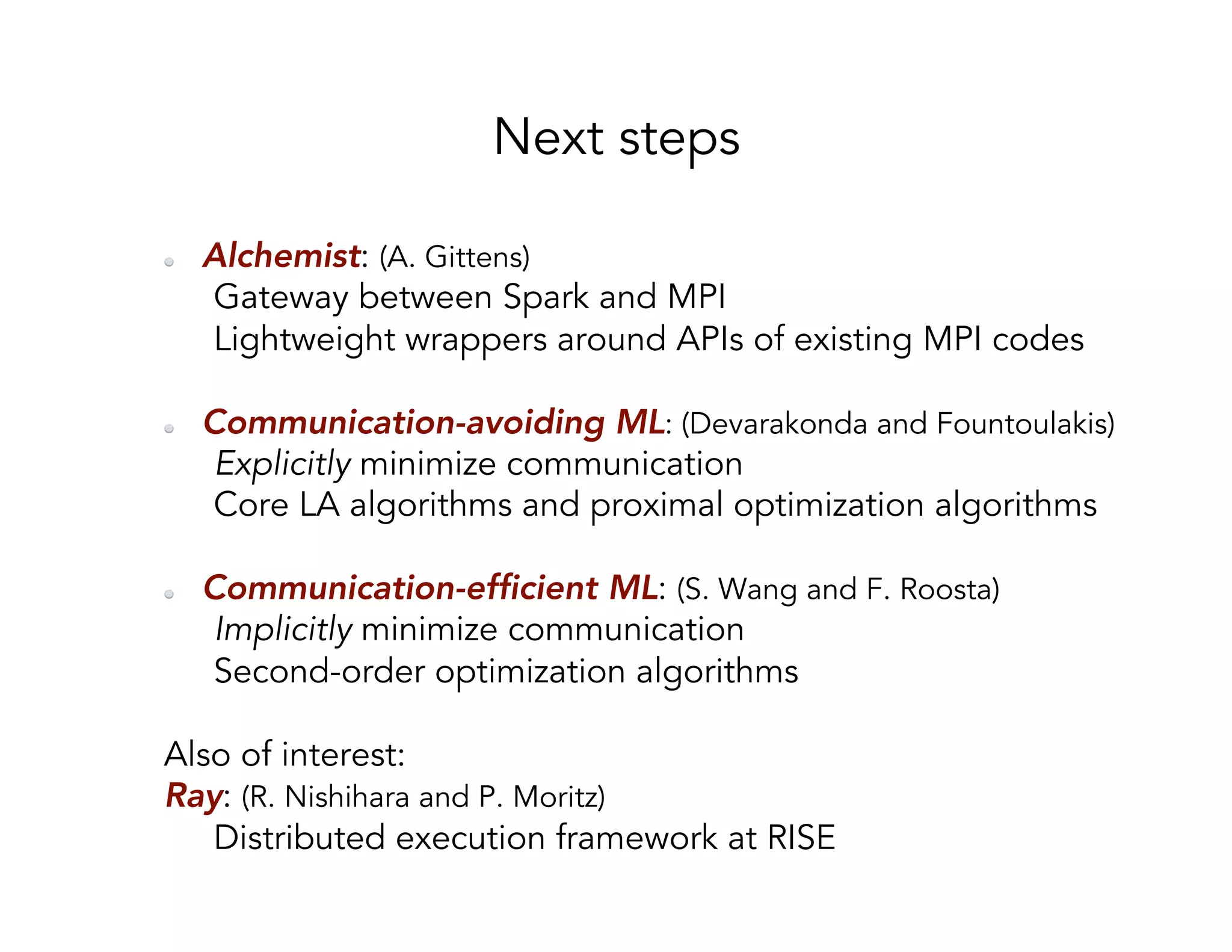
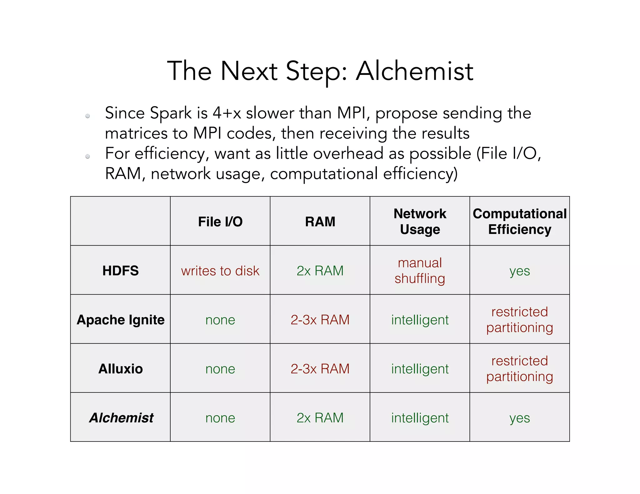
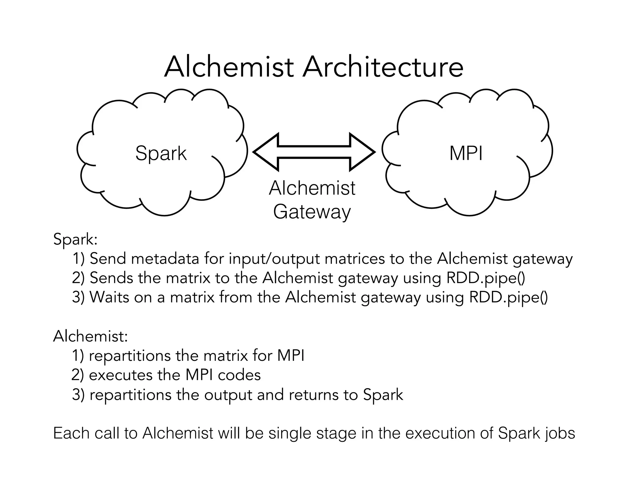
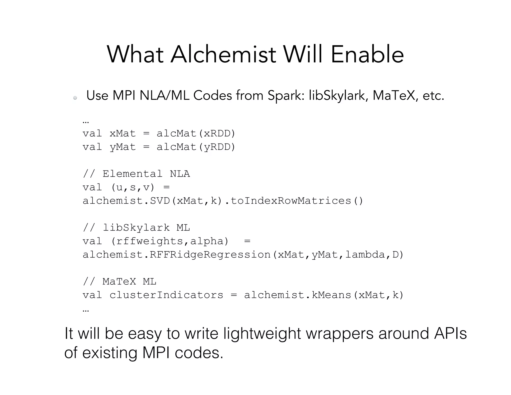
This document discusses computationally intensive machine learning at large scales. It compares the algorithmic and statistical perspectives of computer scientists and statisticians when analyzing big data. It describes three science applications that use linear algebra techniques like PCA, NMF and CX decompositions on large datasets. Experiments are presented comparing the performance of these techniques implemented in Spark and MPI on different HPC platforms. The results show Spark can be 4-26x slower than optimized MPI codes. Next steps proposed include developing Alchemist to interface Spark and MPI more efficiently and exploring communication-avoiding machine learning algorithms.