Downloaded 64 times


![Matlab and polynomials Matlab has a few built-in functions for dealing with polynomials that are worth knowing. An nth order polynomial in Matlab is represented by an array of its n + 1 coefficients: 4x4 + 7x3 + x2 − 2x + 1 » p = [4 7 1 -2 1]; Che 310 — Chapra 17 3 — Interpolation September 7, 2017 3 / 16](https://image.slidesharecdn.com/lecture3-f17-170816220509/75/Lecture-3-Introduction-to-Interpolation-8-2048.jpg)
![Matlab and polynomials Matlab has a few built-in functions for dealing with polynomials that are worth knowing. An nth order polynomial in Matlab is represented by an array of its n + 1 coefficients: 4x4 + 7x3 + x2 − 2x + 1 » p = [4 7 1 -2 1]; The order of the polynomial is 4, so length(p) is 5. Che 310 — Chapra 17 3 — Interpolation September 7, 2017 3 / 16](https://image.slidesharecdn.com/lecture3-f17-170816220509/75/Lecture-3-Introduction-to-Interpolation-9-2048.jpg)
![Matlab and polynomials Matlab has a few built-in functions for dealing with polynomials that are worth knowing. An nth order polynomial in Matlab is represented by an array of its n + 1 coefficients: 4x4 + 7x3 + x2 − 2x + 1 » p = [4 7 1 -2 1]; The order of the polynomial is 4, so length(p) is 5. p(1) is the coefficient of x4. Che 310 — Chapra 17 3 — Interpolation September 7, 2017 3 / 16](https://image.slidesharecdn.com/lecture3-f17-170816220509/75/Lecture-3-Introduction-to-Interpolation-10-2048.jpg)
![Matlab and polynomials Matlab has a few built-in functions for dealing with polynomials that are worth knowing. An nth order polynomial in Matlab is represented by an array of its n + 1 coefficients: 4x4 + 7x3 + x2 − 2x + 1 » p = [4 7 1 -2 1]; The order of the polynomial is 4, so length(p) is 5. p(1) is the coefficient of x4. p(5) is the coefficient of x0 Che 310 — Chapra 17 3 — Interpolation September 7, 2017 3 / 16](https://image.slidesharecdn.com/lecture3-f17-170816220509/75/Lecture-3-Introduction-to-Interpolation-11-2048.jpg)
![Matlab and polynomials Matlab has a few built-in functions for dealing with polynomials that are worth knowing. An nth order polynomial in Matlab is represented by an array of its n + 1 coefficients: 4x4 + 7x3 + x2 − 2x + 1 » p = [4 7 1 -2 1]; The order of the polynomial is 4, so length(p) is 5. p(1) is the coefficient of x4. p(5) is the coefficient of x0 If there are missing terms in a polynomial expression, a 0 must be used in the Matlab representation: x3 + x − 1 » p = [1 0 1 -1]; x5 » p = [1 0 0 0 0]; Che 310 — Chapra 17 3 — Interpolation September 7, 2017 3 / 16](https://image.slidesharecdn.com/lecture3-f17-170816220509/75/Lecture-3-Introduction-to-Interpolation-12-2048.jpg)
![Matlab and polynomials The function polyval can be used to evaluate a polynomial at any number of x-values: 4x4 + 2x3 − 3x2 − 3x + 1 >> x = [ - 1 0 1 ]; >> p = [4 2 -3 -3 1]; >> polyval(p,x) ans = 5 3 1 1 Che 310 — Chapra 17 3 — Interpolation September 7, 2017 4 / 16](https://image.slidesharecdn.com/lecture3-f17-170816220509/75/Lecture-3-Introduction-to-Interpolation-13-2048.jpg)
![Matlab and polynomials The function polyval can be used to evaluate a polynomial at any number of x-values: 4x4 + 2x3 − 3x2 − 3x + 1 >> x = [ - 1 0 1 ]; >> p = [4 2 -3 -3 1]; >> polyval(p,x) ans = 5 3 1 1 The roots function will return all n roots of an nth -order polynomial. (Some roots may contain imaginary numbers) >> r = roots(p) r = -0.84202 + 0.5319i -0.84202 - 0.5319i 5 0.90577 0.27826 >> length(r) ans = 4 Che 310 — Chapra 17 3 — Interpolation September 7, 2017 4 / 16](https://image.slidesharecdn.com/lecture3-f17-170816220509/75/Lecture-3-Introduction-to-Interpolation-14-2048.jpg)
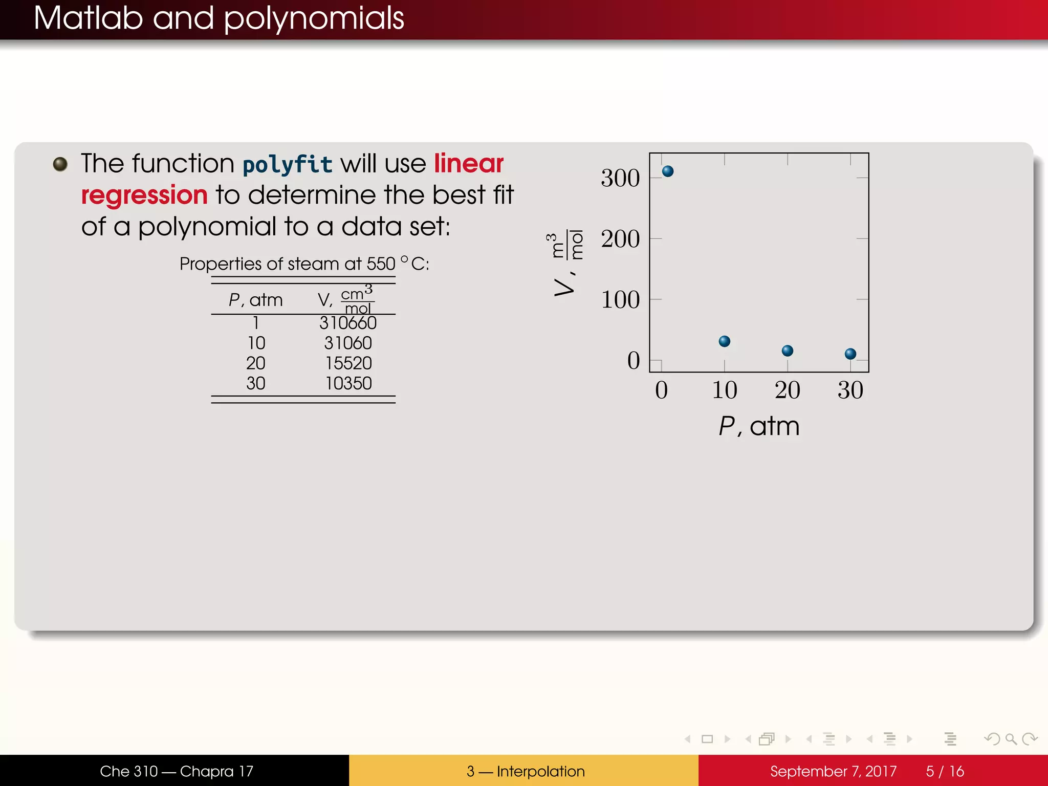
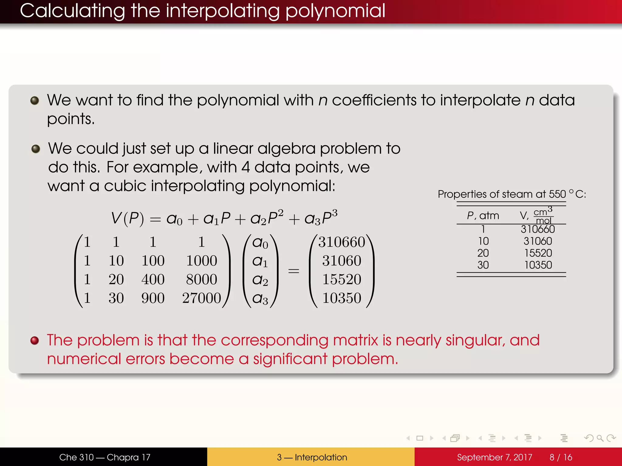
![Matlab and polynomials The function polyfit will use linear regression to determine the best fit of a polynomial to a data set: Properties of steam at 550 ◦ C: P, atm V, cm3 mol 1 310660 10 31060 20 15520 30 10350 >> logP = [1,10,20,30]; >> V = [310660,31060,15520,10350]; >> order = 2; >> p = polyfit(logP,V,order); >> fplot(@(x)polyval(p,x),[0 30],’r’); 0 10 20 30 0 100 200 300 P, atm V,m3 mol If order < length(logP)-1 then linear regression is used. Che 310 — Chapra 17 3 — Interpolation September 7, 2017 5 / 16](https://image.slidesharecdn.com/lecture3-f17-170816220509/75/Lecture-3-Introduction-to-Interpolation-16-2048.jpg)
![Matlab and polynomials The function polyfit will use linear regression to determine the best fit of a polynomial to a data set: Properties of steam at 550 ◦ C: P, atm V, cm3 mol 1 310660 10 31060 20 15520 30 10350 >> logP = [1,10,20,30]; >> V = [310660,31060,15520,10350]; >> order = 3; >> p = polyfit(logP,V,order); >> fplot(@(x)polyval(p,x),[0 30],’g’); 0 10 20 30 0 200 400 P, atm V,m3 mol If order < length(logP)-1 then linear regression is used. If order == length(logP)-1 then the interpolating polynomial is calculated. Che 310 — Chapra 17 3 — Interpolation September 7, 2017 5 / 16](https://image.slidesharecdn.com/lecture3-f17-170816220509/75/Lecture-3-Introduction-to-Interpolation-17-2048.jpg)
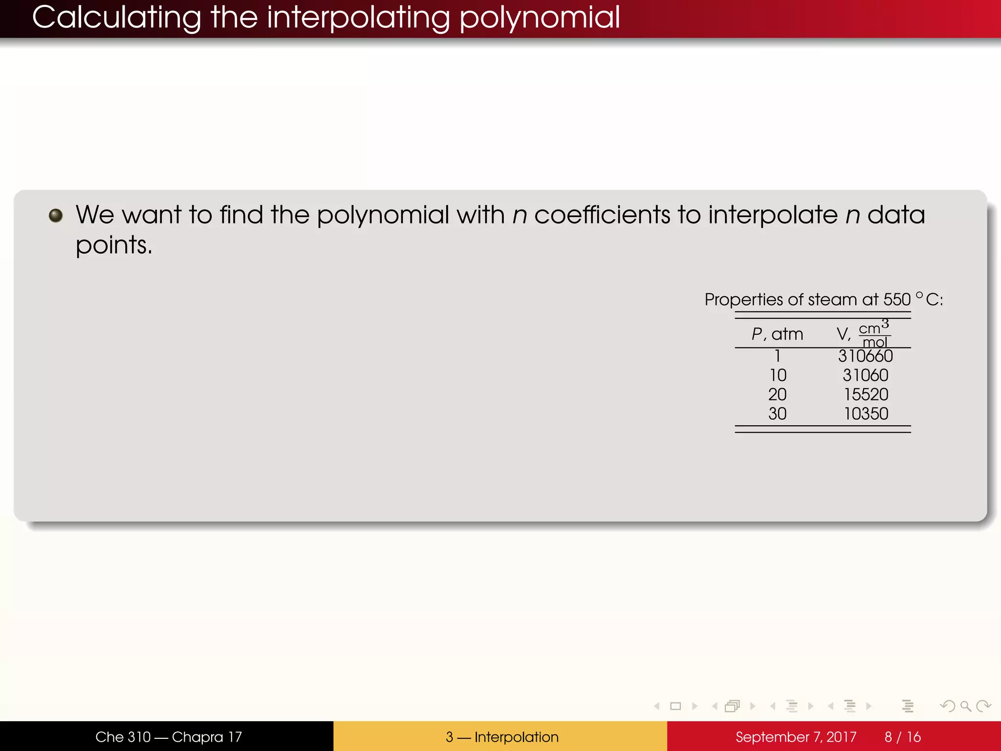
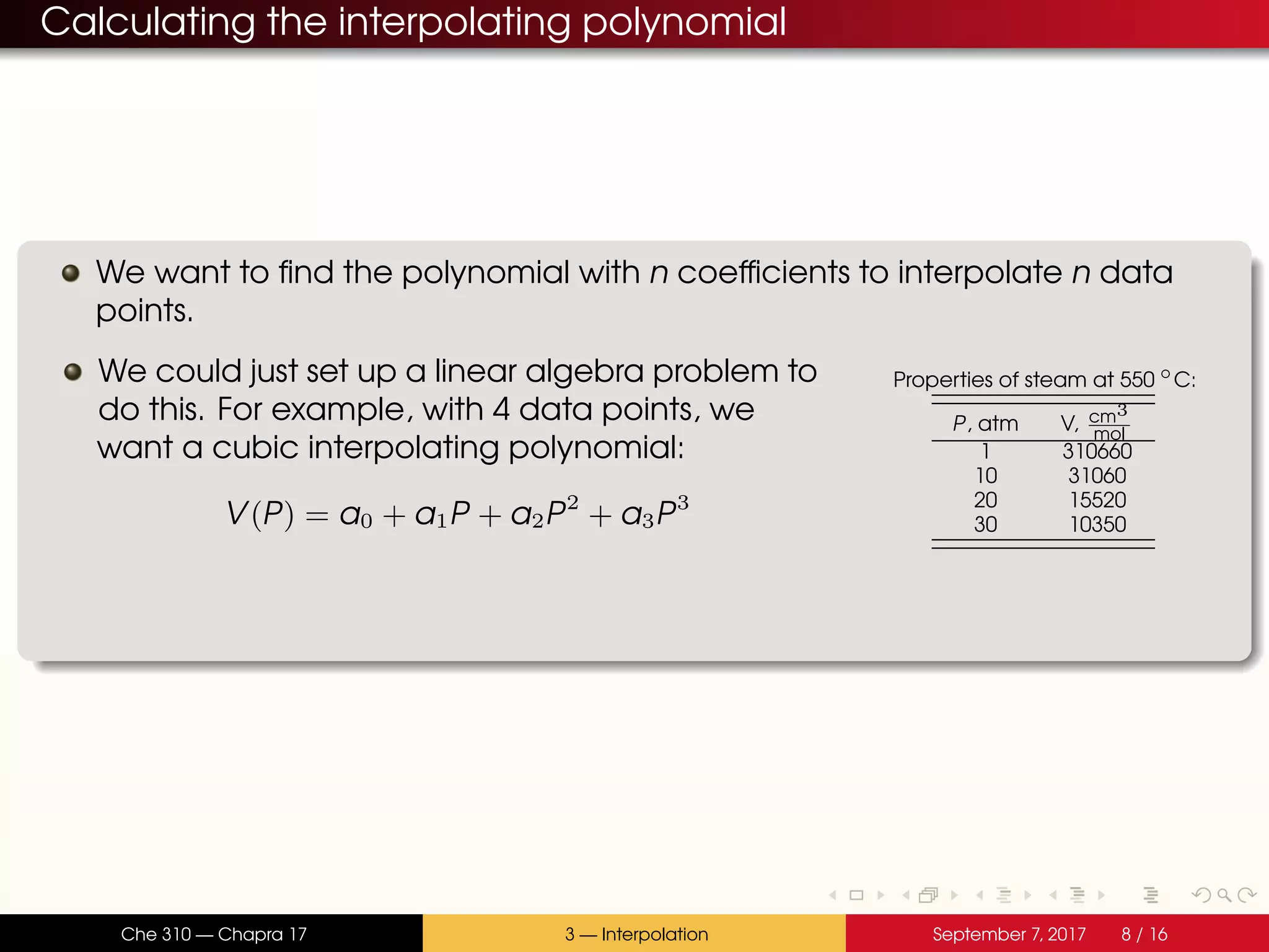
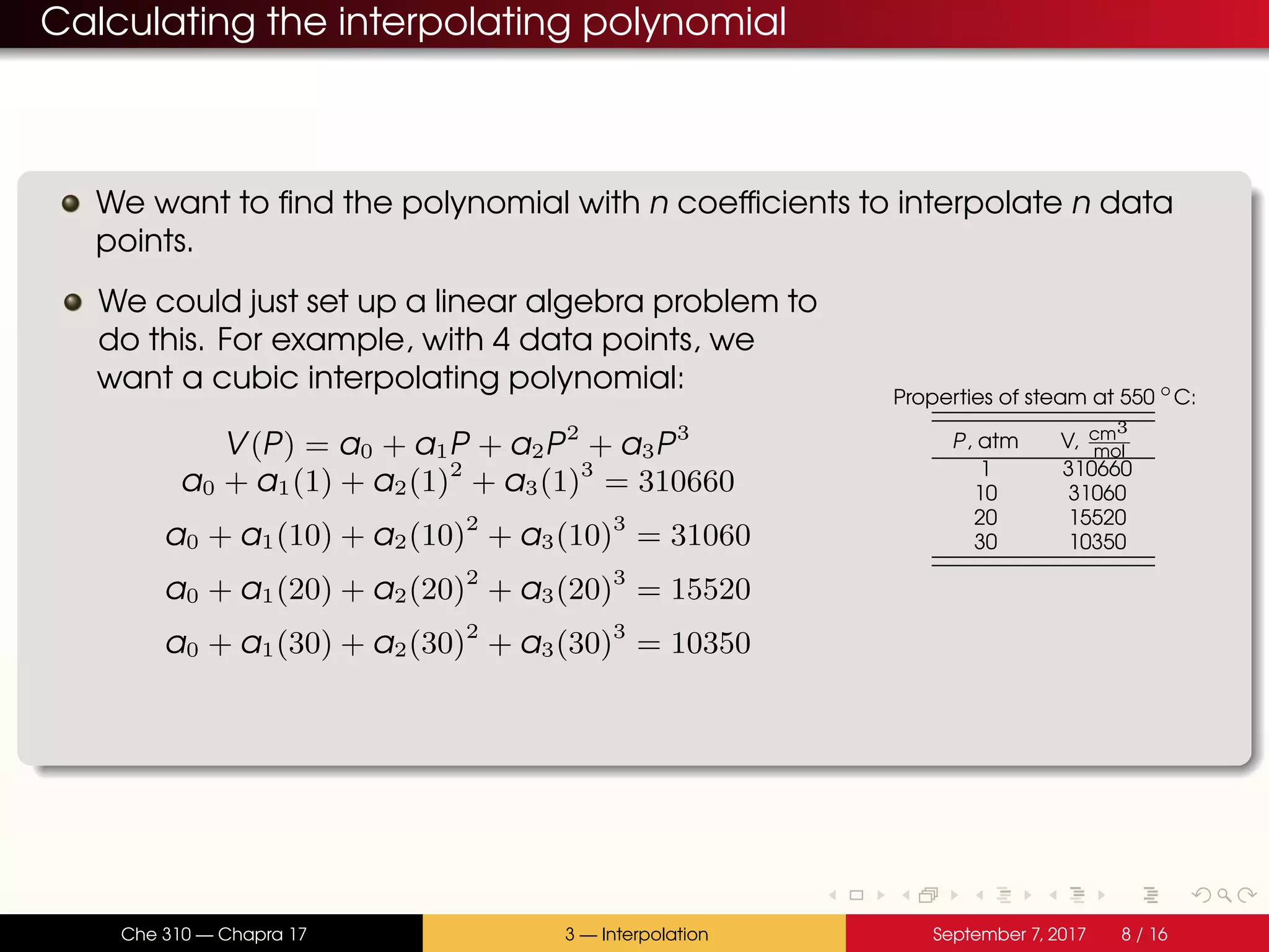
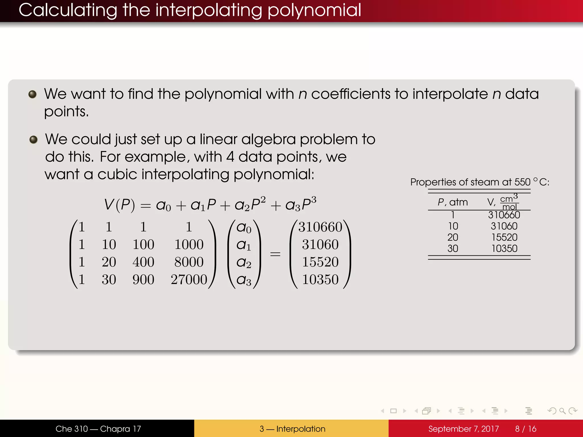
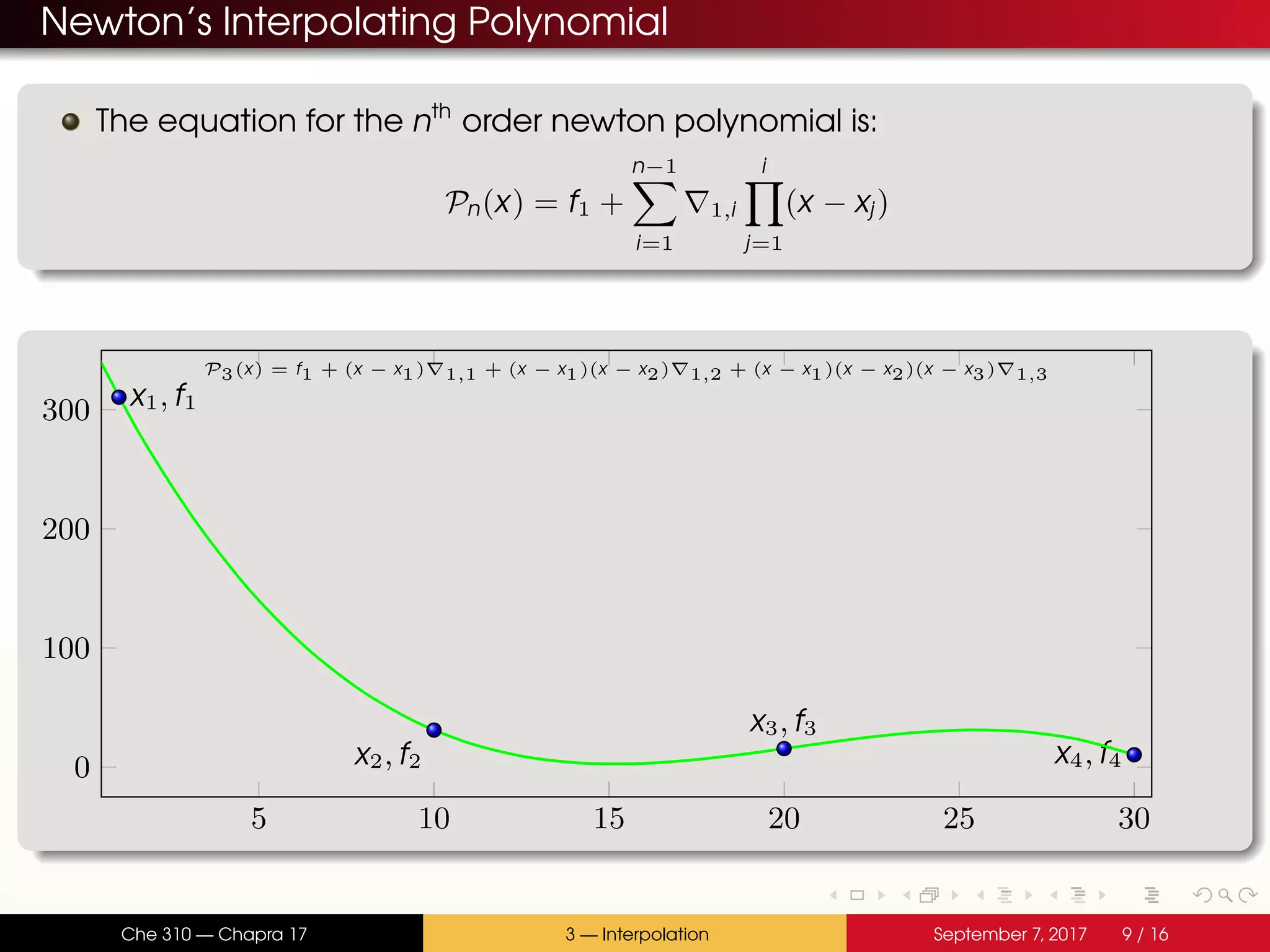
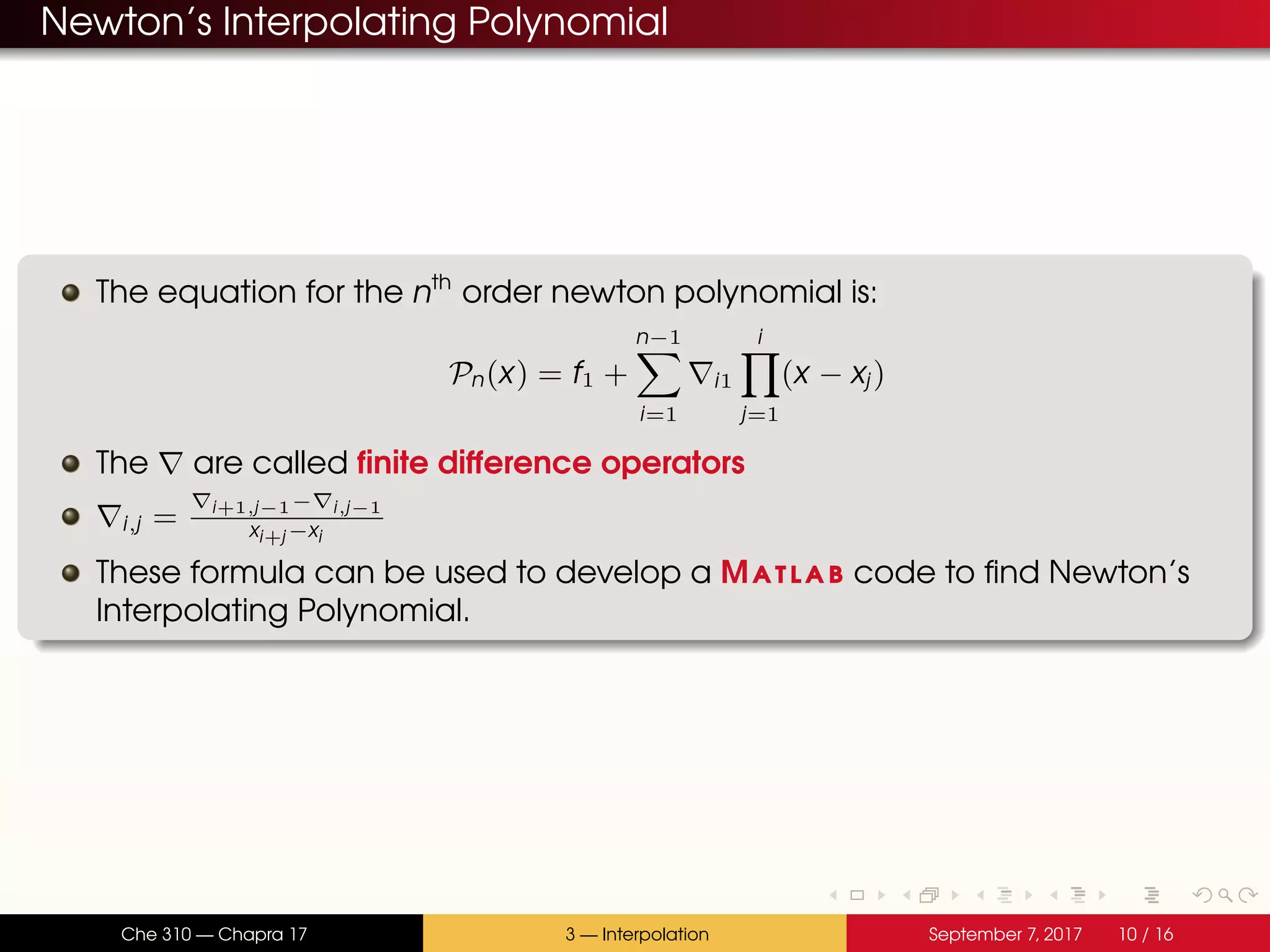
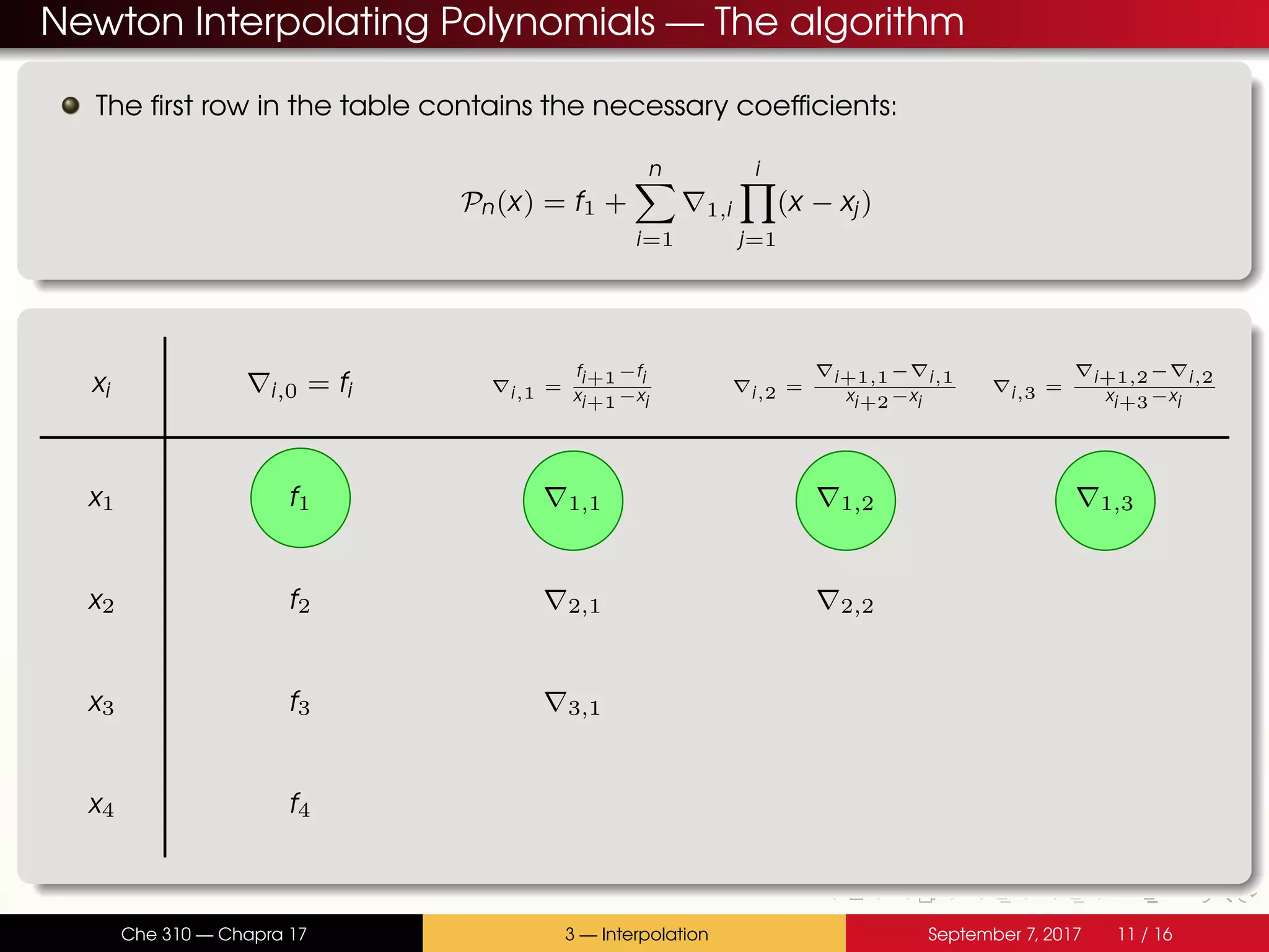
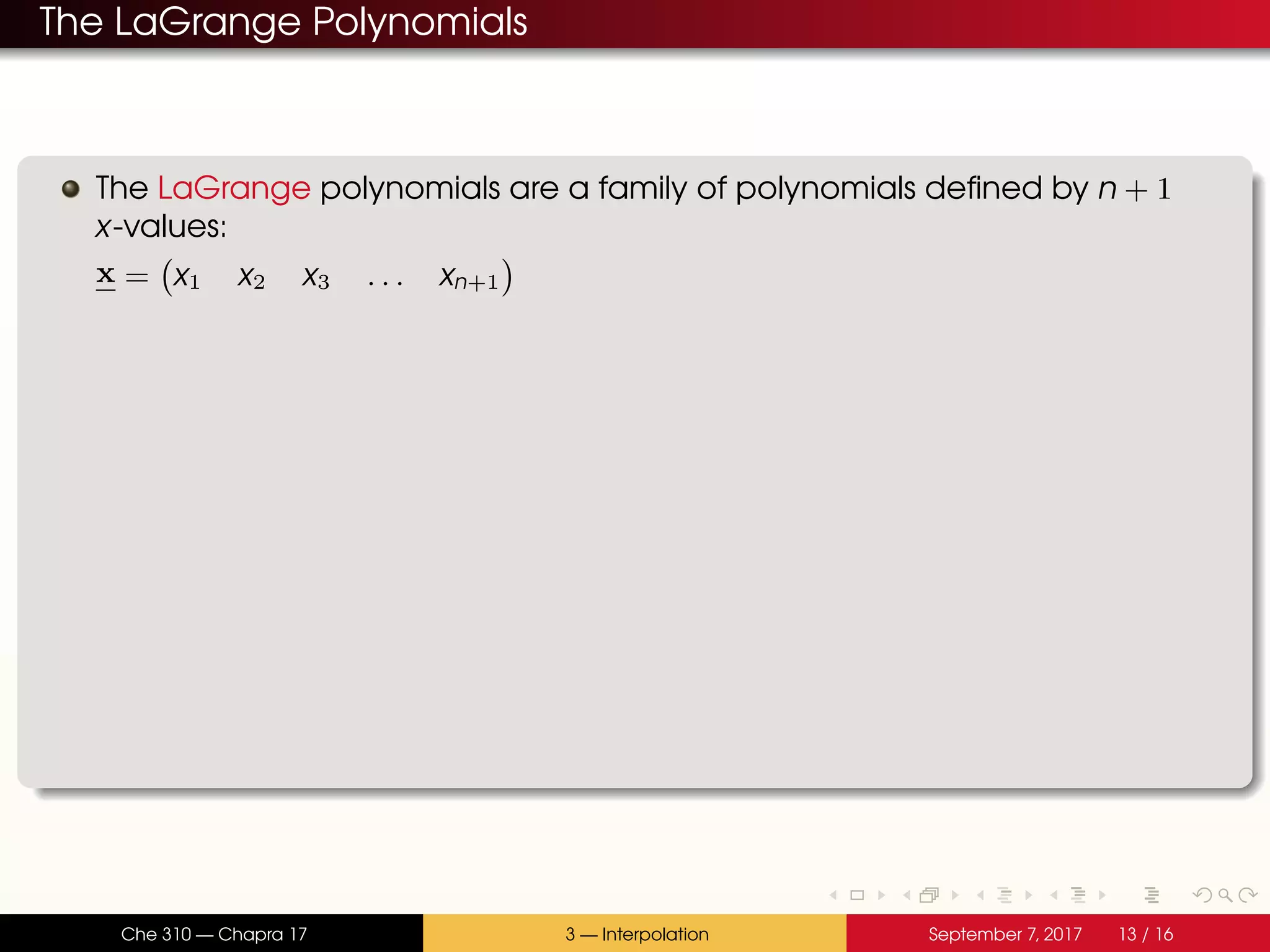
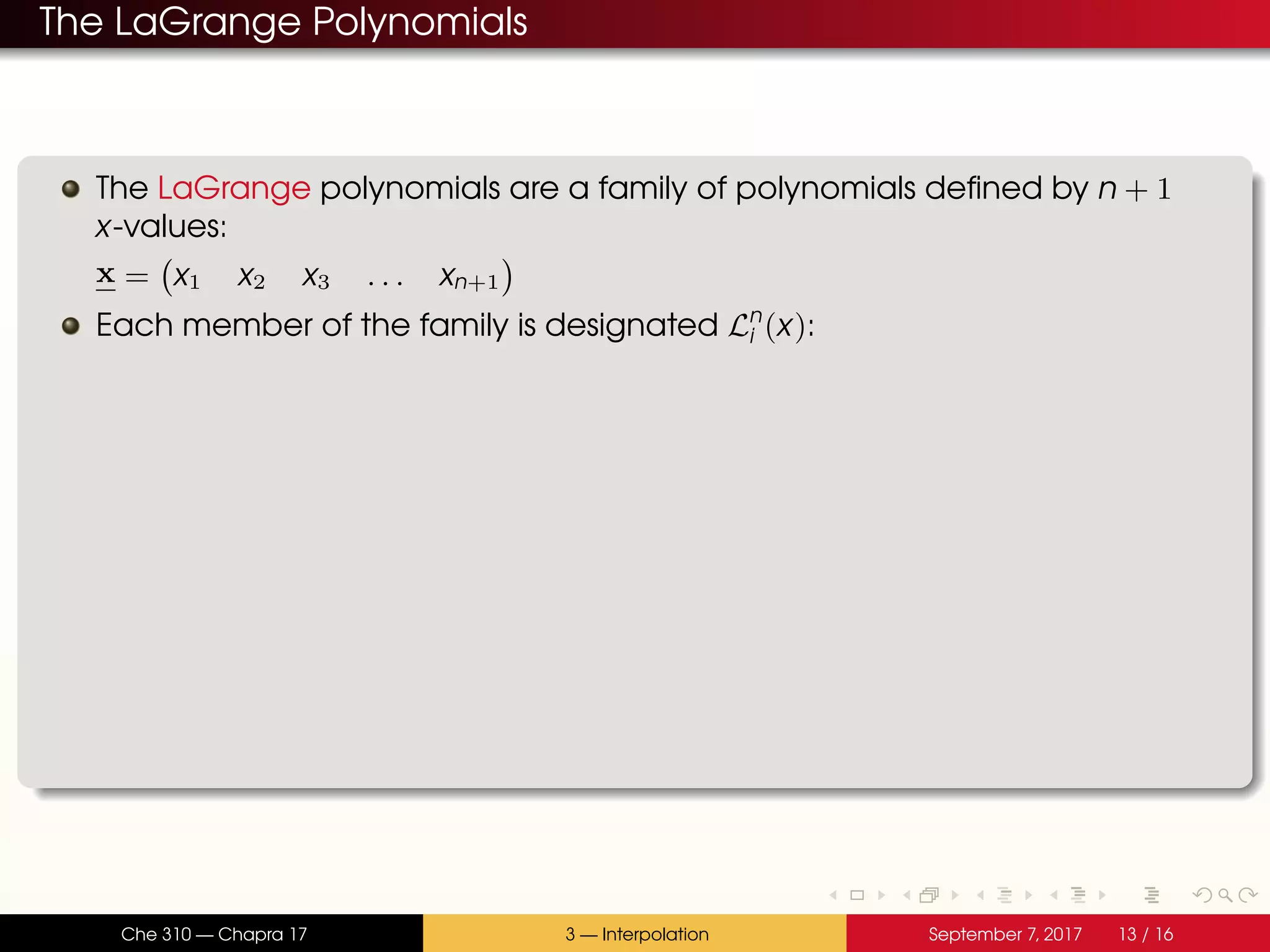
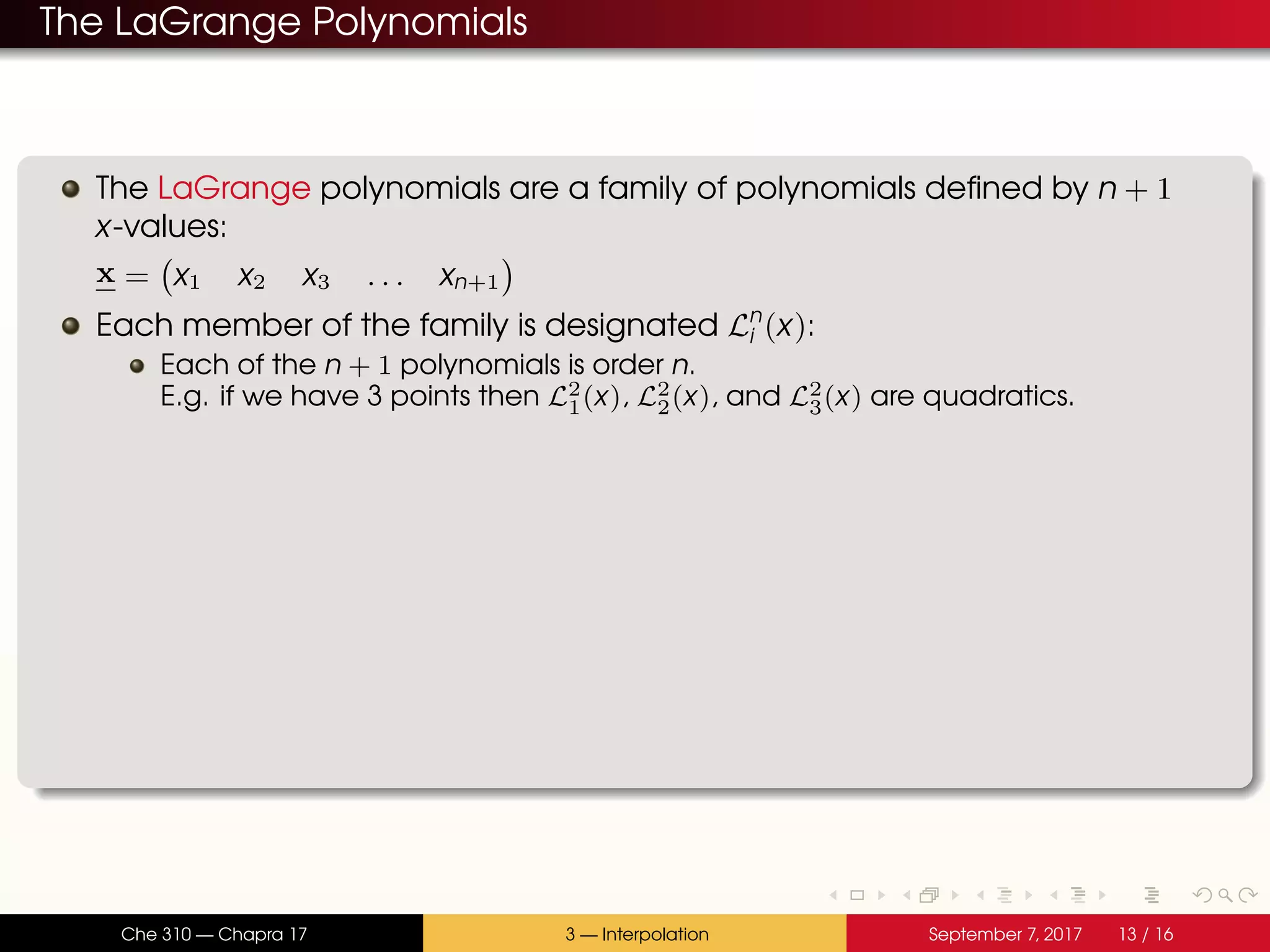
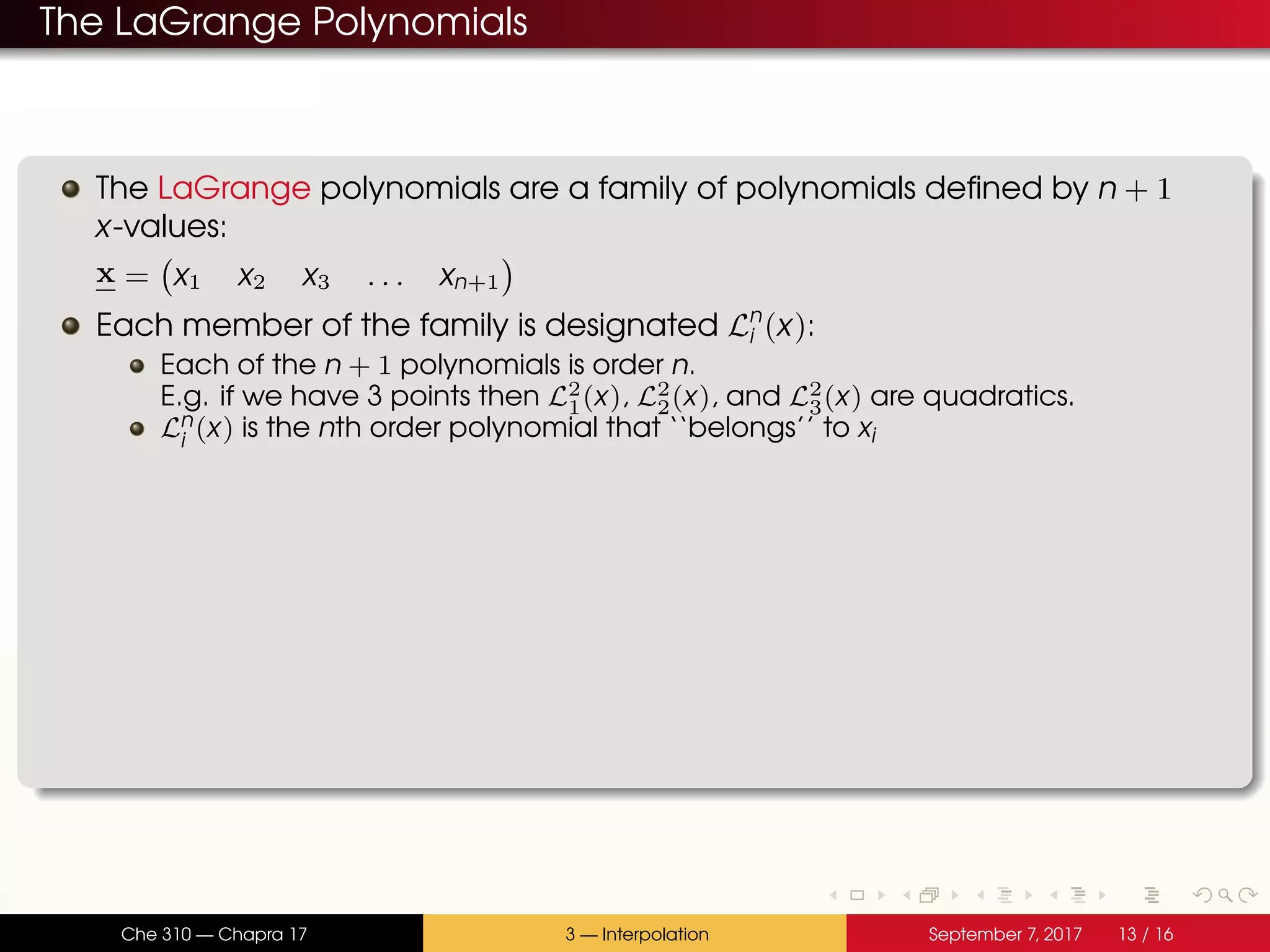
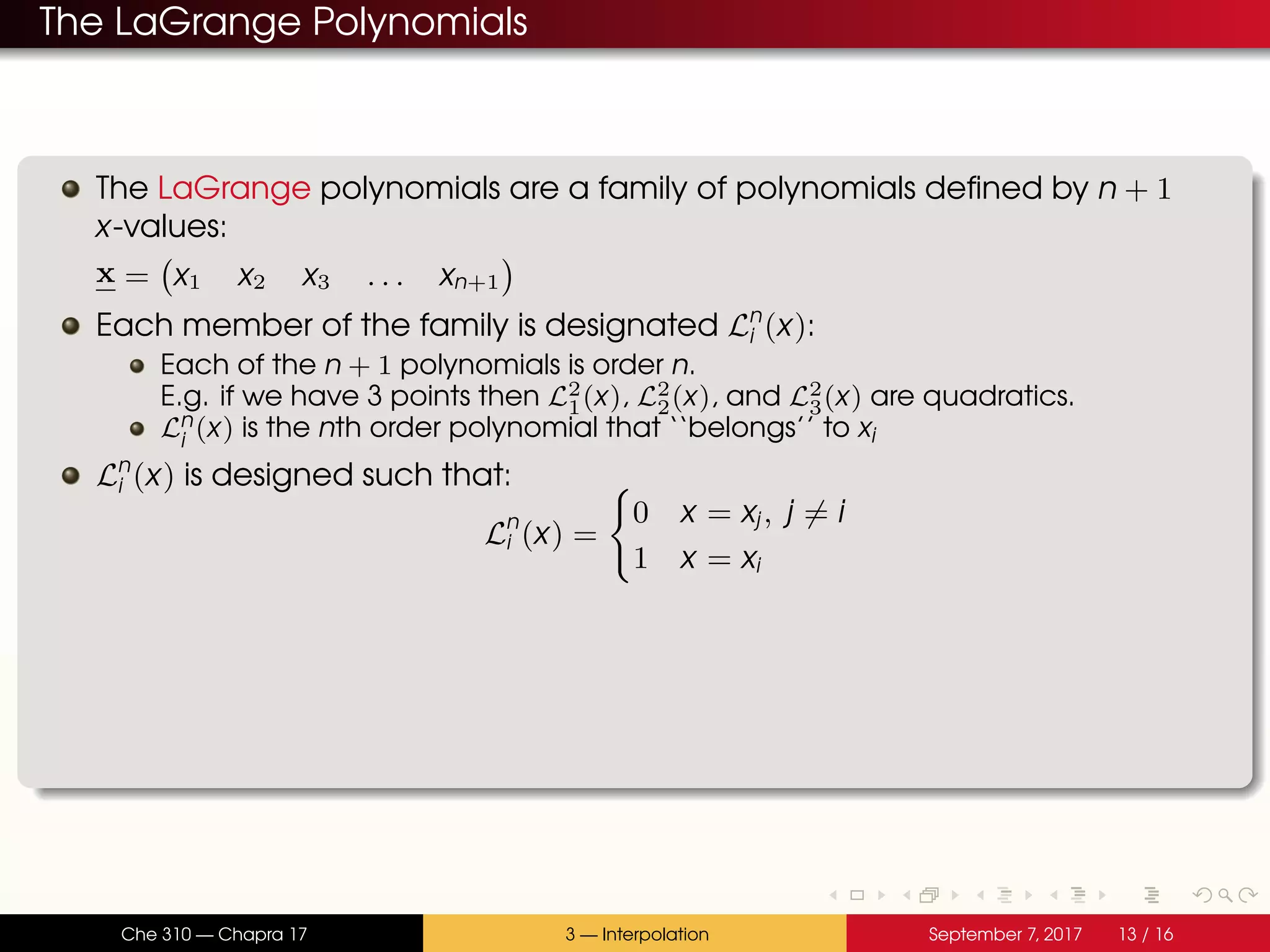
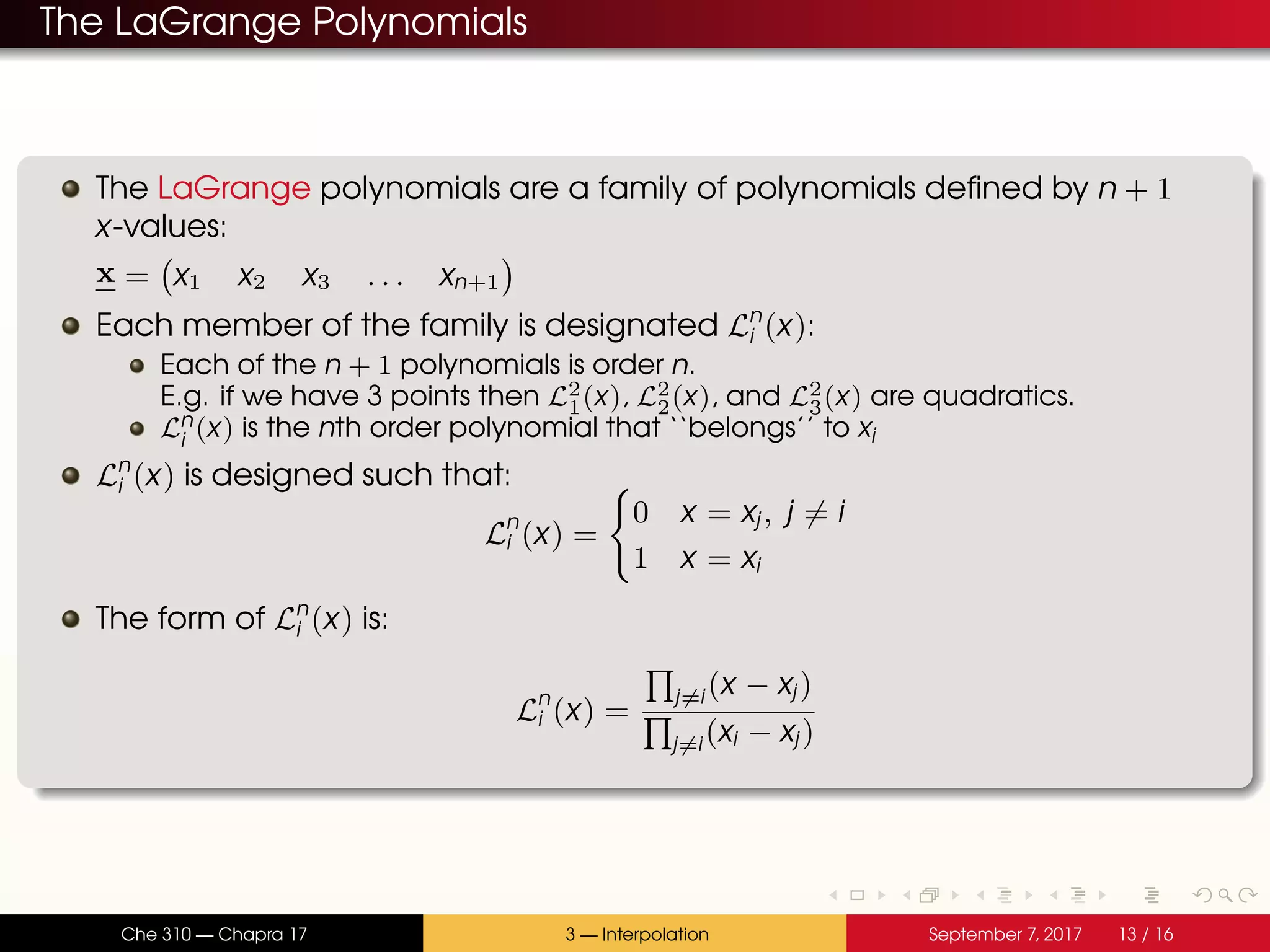
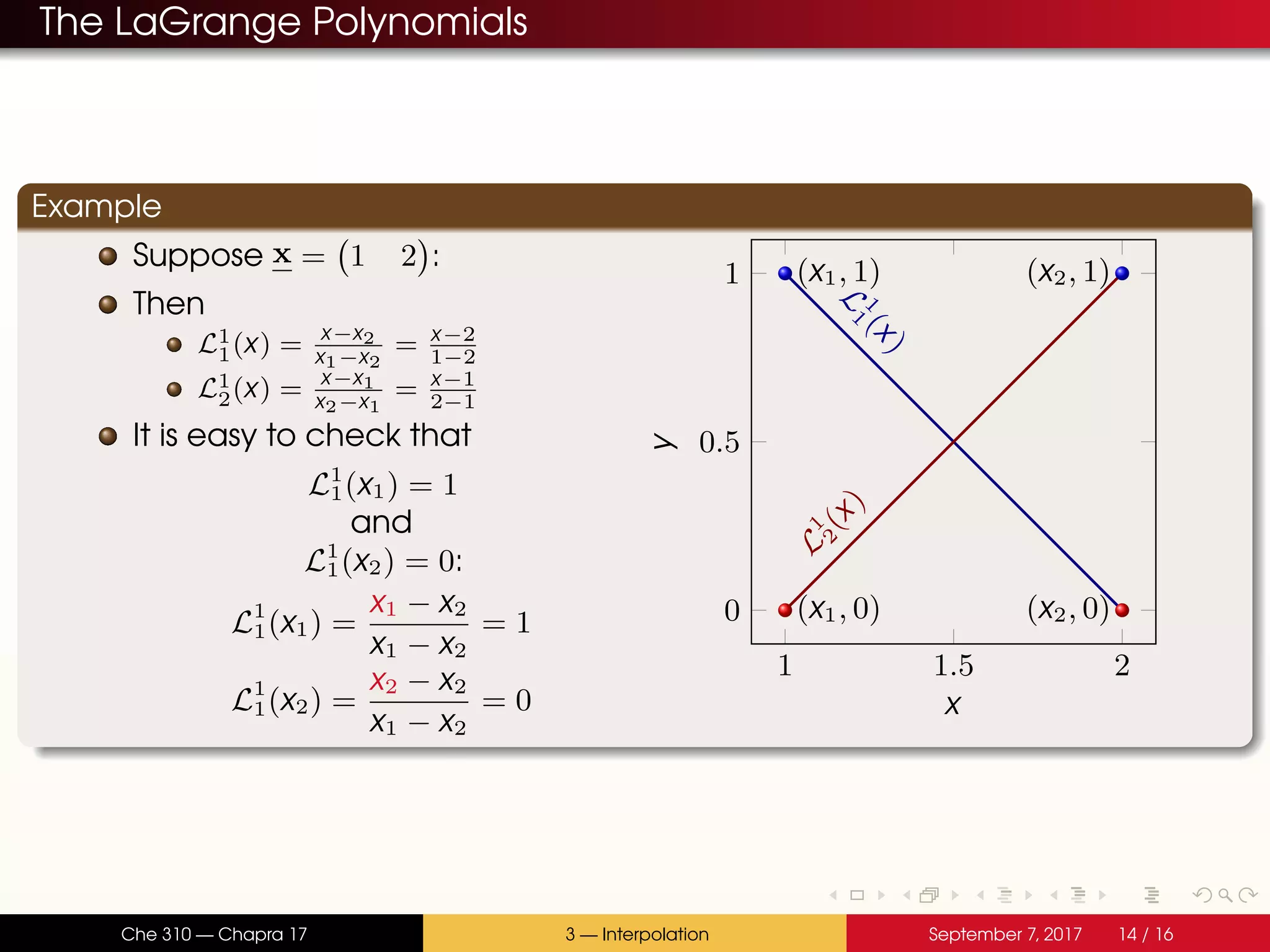
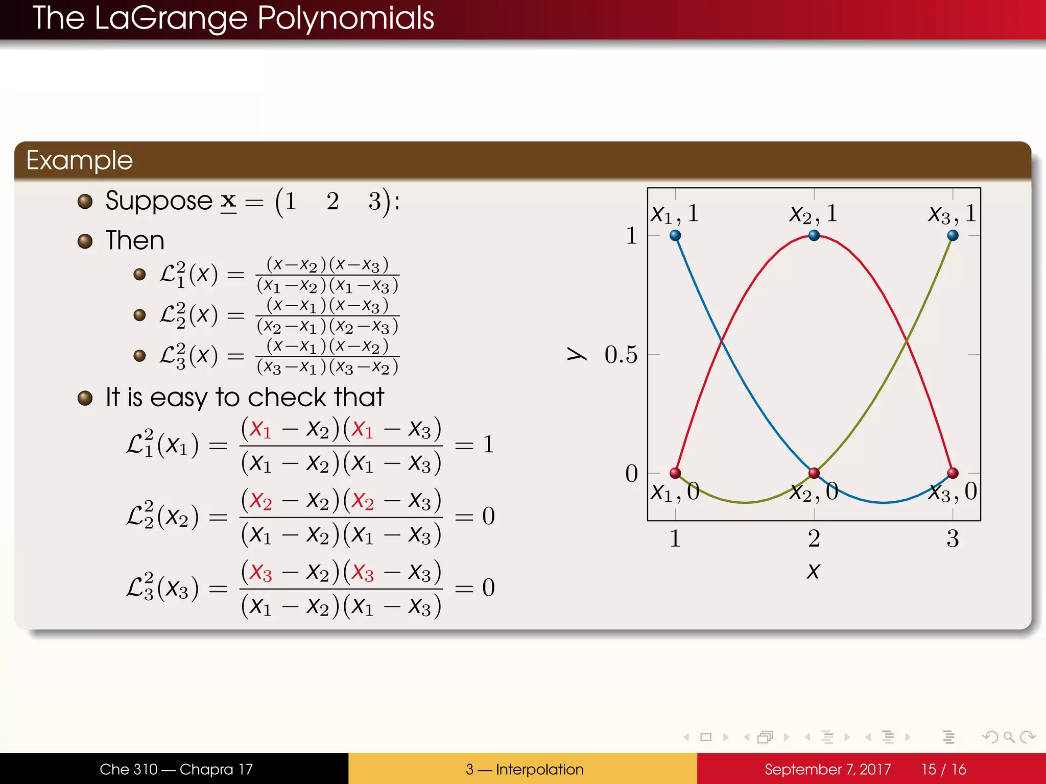
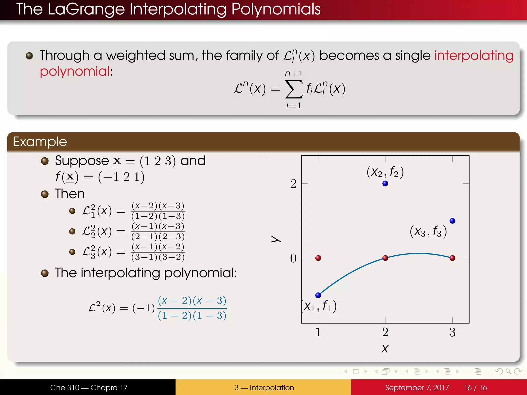
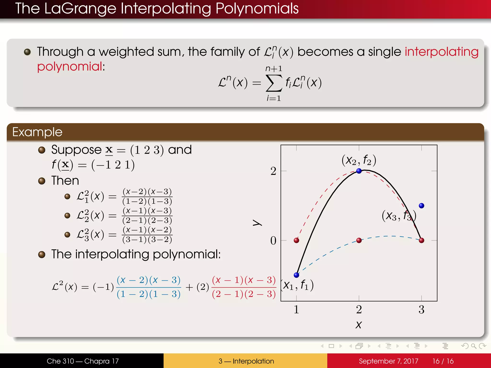
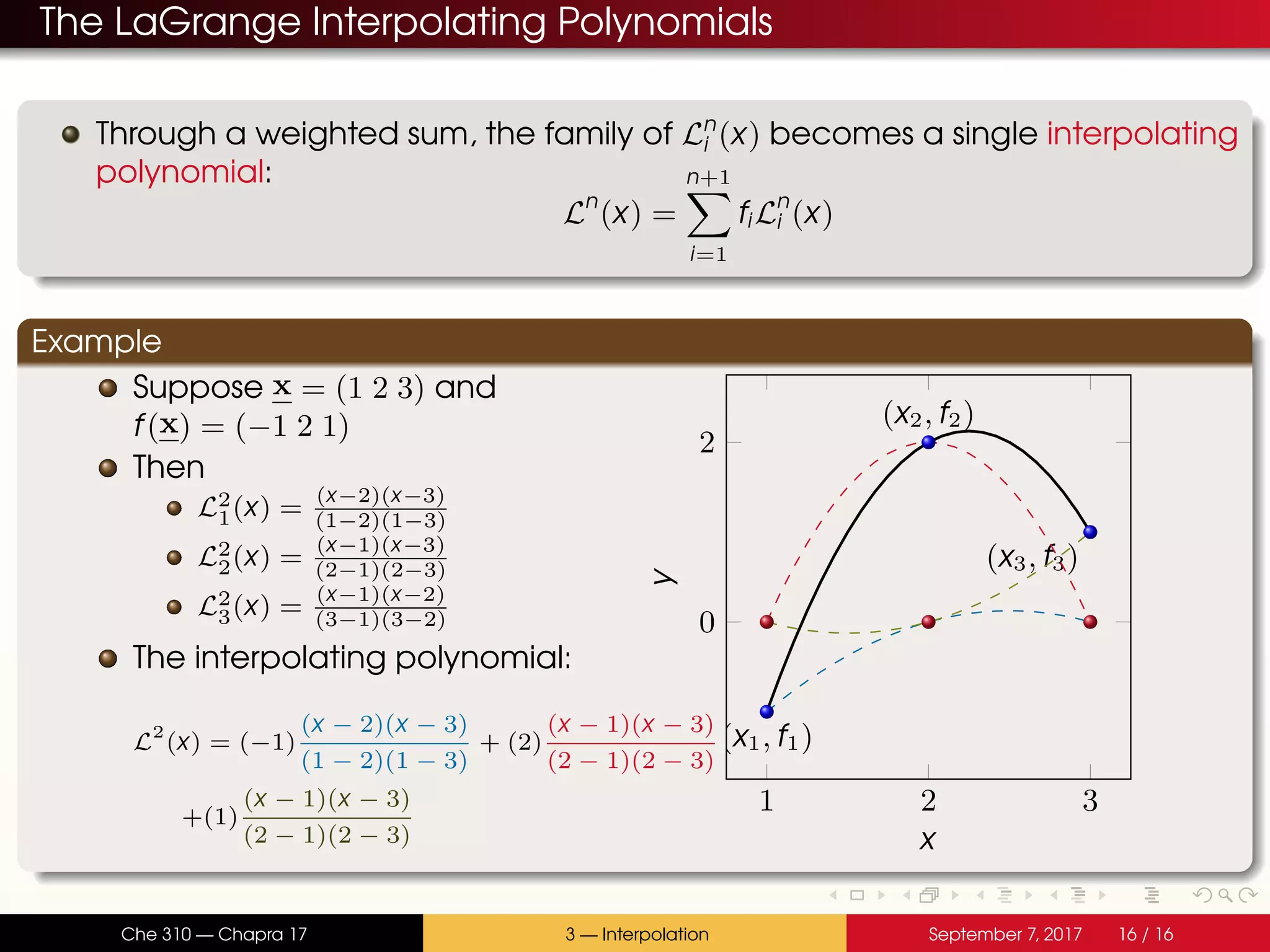

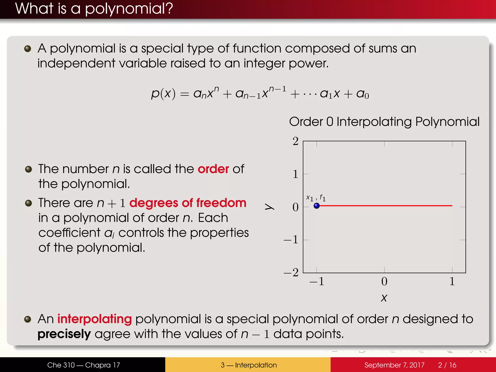
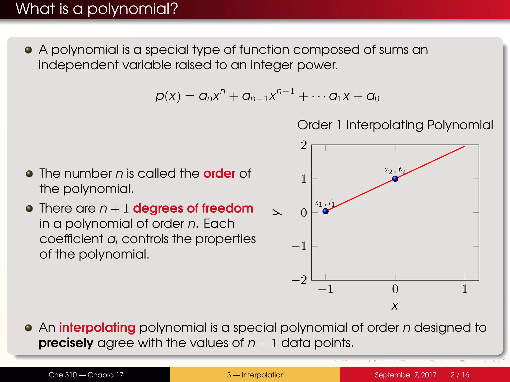
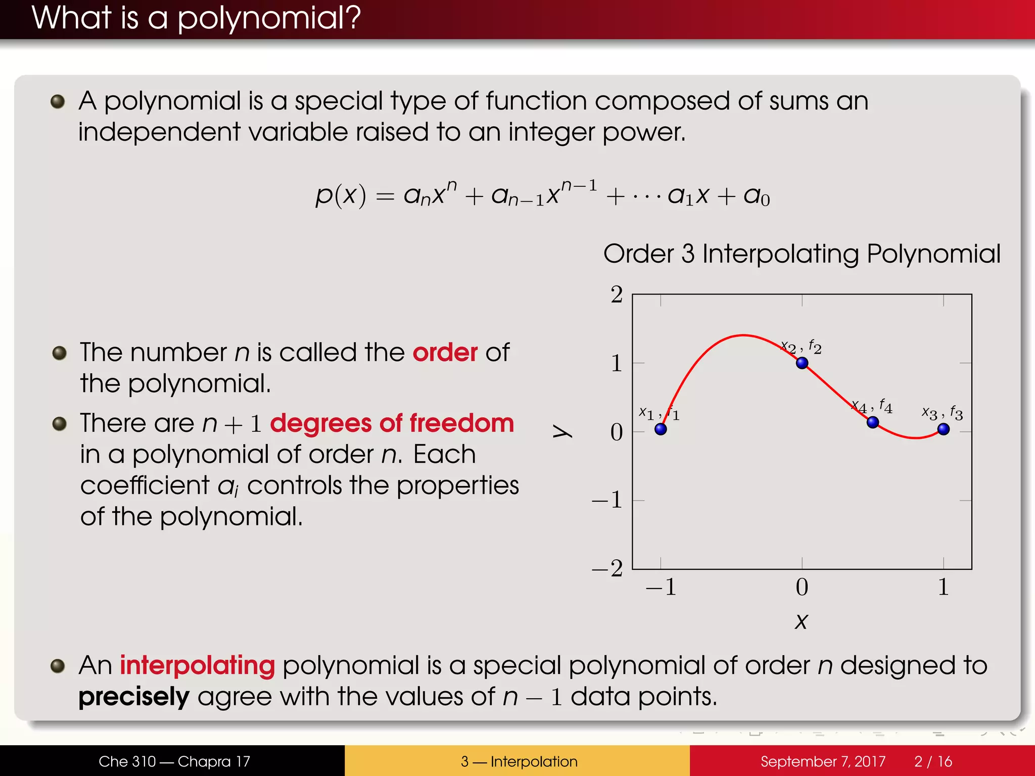
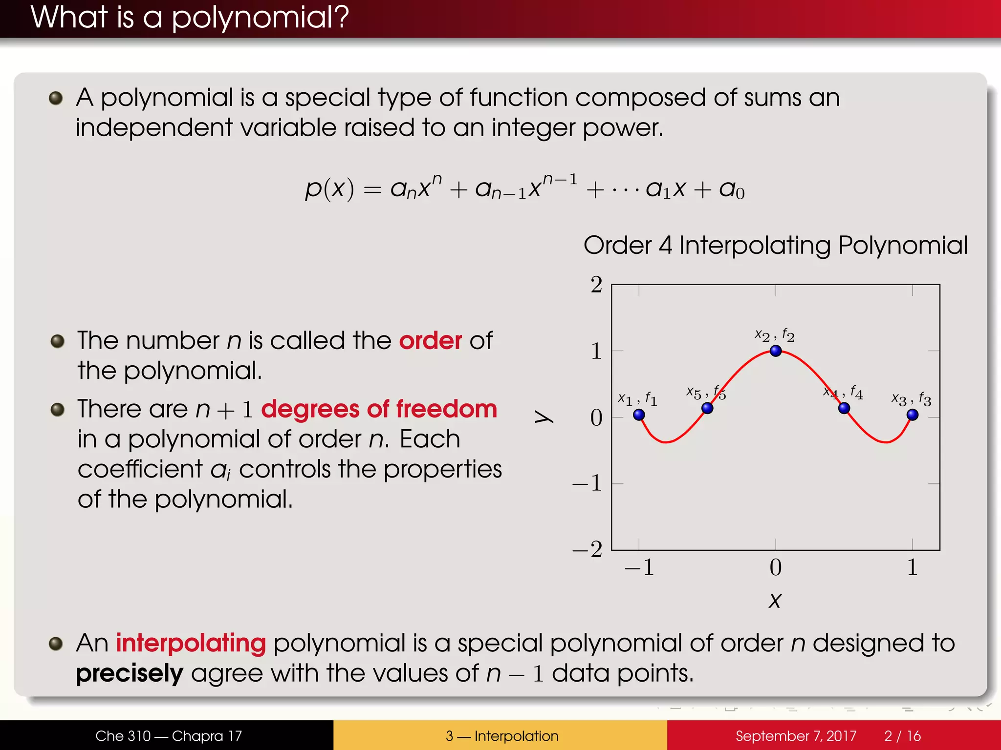
The document discusses polynomial interpolation. It begins by defining polynomials and interpolating polynomials. Interpolating polynomials are polynomials of order n that precisely fit n data points. The document then discusses how Matlab can be used to generate, evaluate, and find properties of polynomials. Specifically, it describes how the polyfit, polyval, and roots functions work. Finally, it discusses two methods for generating interpolating polynomials: Newton and Lagrange polynomials. The key application of interpolating polynomials is estimating values within tabulated data points.