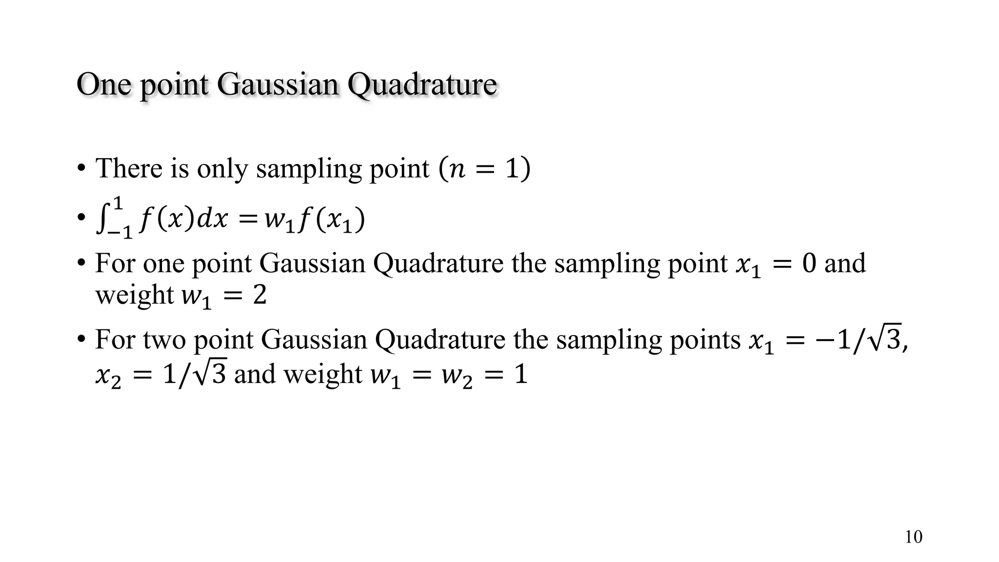
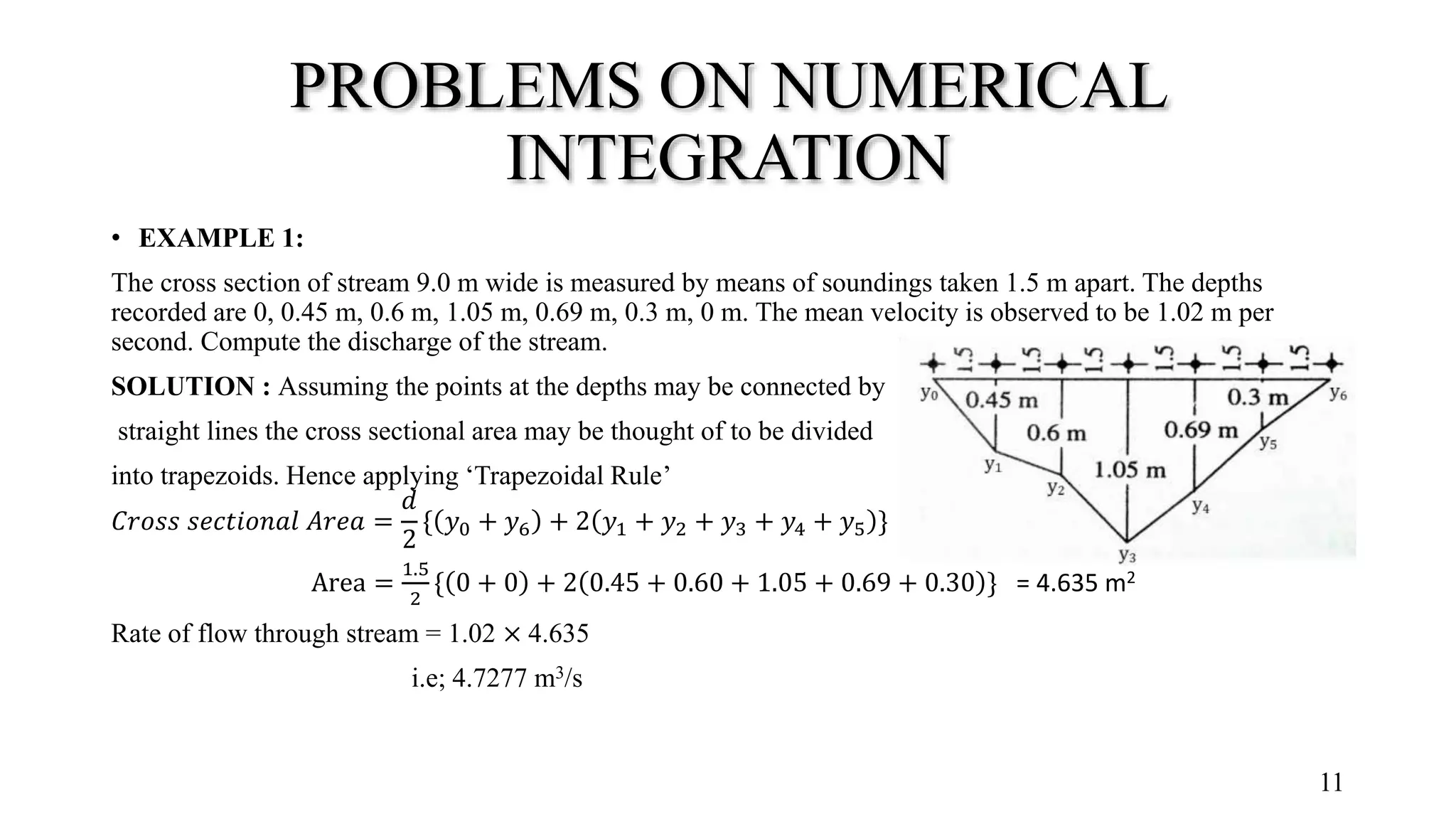
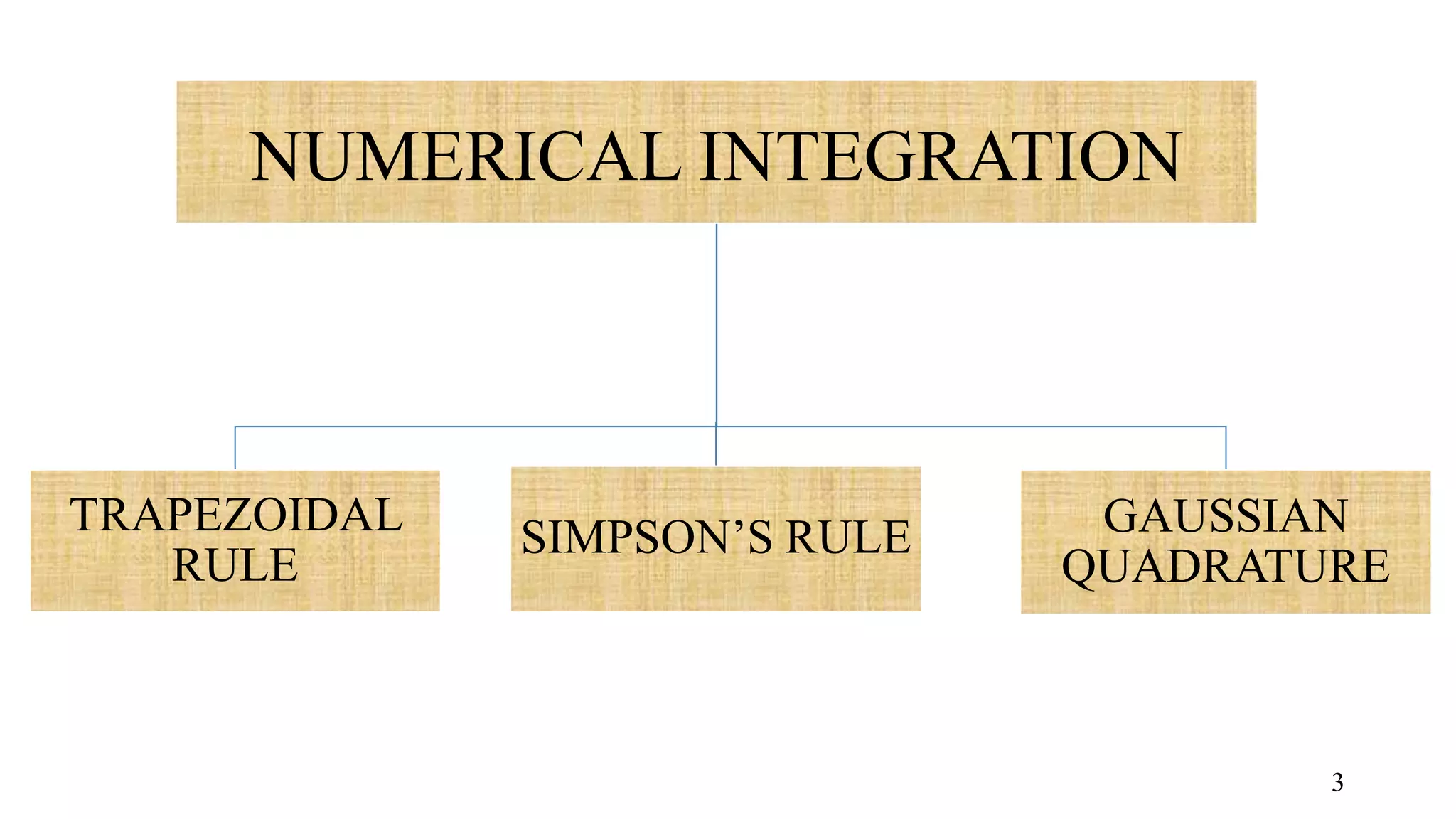
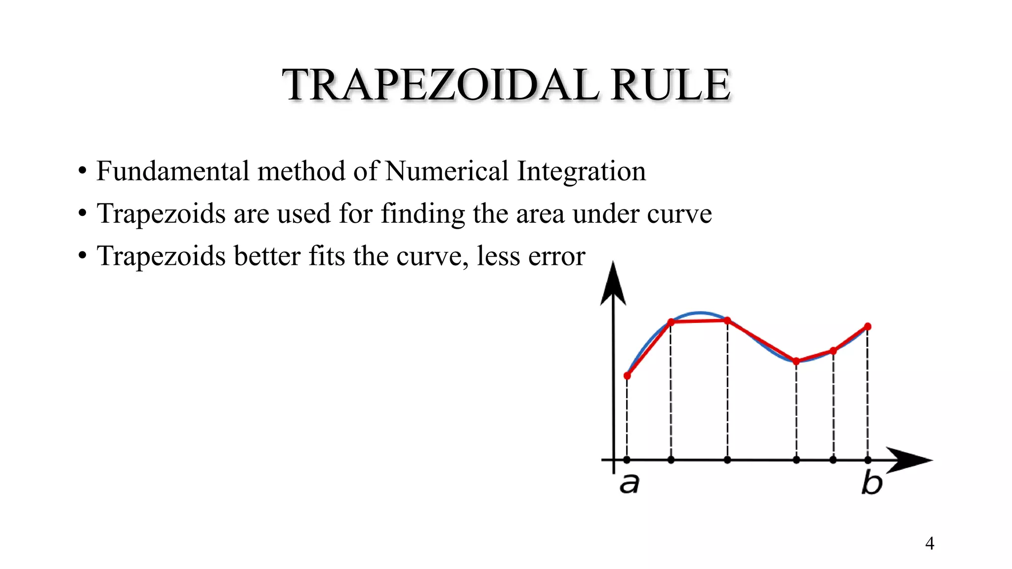
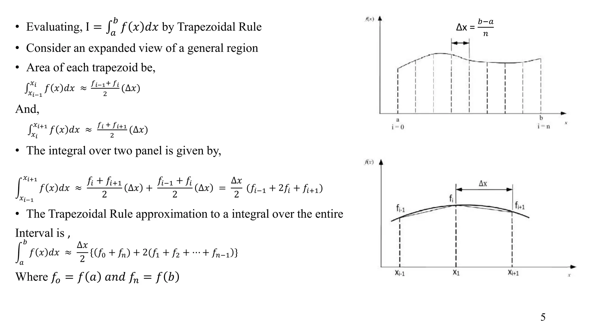
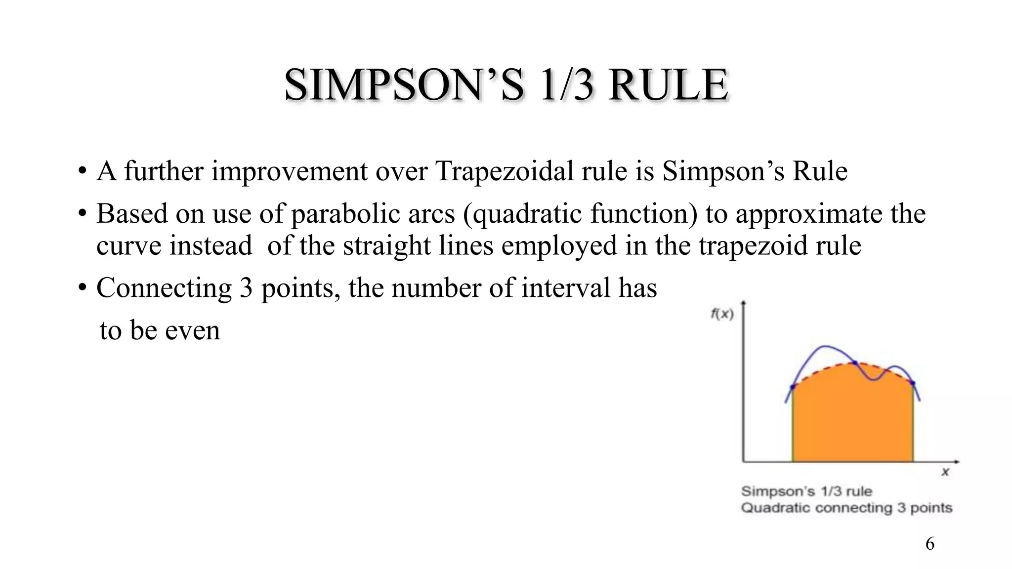
Numerical Integration BY TAUSIF SHAHANSHAH BCE – 3rd YEAR DEPT. OF CIVIL ENGG. JADAVPUR UNIVERSITY 1
WHAT IS NUMERICAL INTEGRATION? • Approximate computation of a definite integral using numerical techniques • Tabulated at regularly spaced intervals • Gives the approximate calculation • Different from analytical integration 2
NUMERICAL INTEGRATION TRAPEZOIDAL RULE SIMPSON’S RULE GAUSSIAN QUADRATURE 3
TRAPEZOIDAL RULE • Fundamental method of Numerical Integration • Trapezoids are used for finding the area under curve • Trapezoids better fits the curve, less error 4
• Evaluating, I = 𝑎 𝑏 𝑓 𝑥 𝑑𝑥 by Trapezoidal Rule • Consider an expanded view of a general region • Area of each trapezoid be, 𝑥 𝑖−1 𝑥 𝑖 𝑓 𝑥 𝑑𝑥 ≈ 𝑓 𝑖−1+ 𝑓 𝑖 2 (∆𝑥) And, 𝑥 𝑖 𝑥 𝑖+1 𝑓 𝑥 𝑑𝑥 ≈ 𝑓 𝑖 + 𝑓 𝑖+1 2 (∆𝑥) • The integral over two panel is given by, 𝑥 𝑖−1 𝑥 𝑖+1 𝑓 𝑥 𝑑𝑥 ≈ 𝑓𝑖 + 𝑓𝑖+1 2 ∆𝑥 + 𝑓𝑖−1 + 𝑓𝑖 2 ∆𝑥 = ∆𝑥 2 (𝑓𝑖−1 + 2𝑓𝑖 + 𝑓𝑖+1) • The Trapezoidal Rule approximation to a integral over the entire Interval is , 𝑎 𝑏 𝑓 𝑥 𝑑𝑥 ≈ ∆𝑥 2 { 𝑓0 + 𝑓𝑛) + 2(𝑓1 + 𝑓2 + ⋯ + 𝑓𝑛−1 } Where 𝑓𝑜 = 𝑓 𝑎 𝑎𝑛𝑑 𝑓𝑛 = 𝑓 𝑏 ∆x = 𝑏−𝑎 𝑛 5
SIMPSON’S 1/3 RULE • A further improvement over Trapezoidal rule is Simpson’s Rule • Based on use of parabolic arcs (quadratic function) to approximate the curve instead of the straight lines employed in the trapezoid rule • Connecting 3 points, the number of interval has to be even 6
• Approximating the area of the panel by the area under the parabola is given by, 𝑥 𝑖−1 𝑥 𝑖+1 𝑓2 𝑥 𝑑𝑥 = ∆𝑥 3 [ 𝑓 𝑥𝑖−1 + 4𝑓 𝑥𝑖 + 𝑓(𝑥𝑖+1)] • The Simpson’s rule approximation to the integral over the entire interval is 𝑎 𝑏 𝑓 𝑥 𝑑𝑥 ≈ ∆𝑥 3 𝑓0 + 4𝑓1 + 2𝑓2 + 4𝑓3 + ⋯ + 2𝑓𝑛−2 + 4𝑓𝑛−1 + 𝑓𝑛 Where 𝑓𝑜 = 𝑓 𝑎 𝑎𝑛𝑑 𝑓𝑛 = 𝑓 𝑏 7
SIMPSON’S 3/8 RULE • Consists of taking the area under a cubic equation connecting four points. • Number of interval must be multiple of three • The formula for Simpson’s 3/8 rule is 𝑎 𝑏 𝑓 𝑥 𝑑𝑥 = 3∆𝑥 8 [ 𝑓0 + 𝑓𝑛 + 2 𝑓3 + 𝑓6 + ⋯ + 𝑓𝑛−3 +3 𝑓1 + 𝑓2 + 𝑓4 + 𝑓5 + ⋯ + 𝑓𝑛−1 ] 8
GAUSSIAN QUADRATURE • Sampling points may not be equally spaced in practical problems • Both positions of the sampling points and the weights have been optimized • Gaussian Quadrature formula can be expressed as, −1 1 𝑓 𝑥 𝑑𝑥 = 𝑖=1 𝑛 𝑤𝑖 𝑓(𝑥𝑖) • It produces most accurate approximation 9
One point Gaussian Quadrature • There is only sampling point 𝑛 = 1 • −1 1 𝑓 𝑥 𝑑𝑥 = 𝑤1 𝑓(𝑥1) • For one point Gaussian Quadrature the sampling point 𝑥1 = 0 and weight 𝑤1 = 2 • For two point Gaussian Quadrature the sampling points 𝑥1 = −1/ 3, 𝑥2 = 1/ 3 and weight 𝑤1 = 𝑤2 = 1 10
PROBLEMS ON NUMERICAL INTEGRATION • EXAMPLE 1: The cross section of stream 9.0 m wide is measured by means of soundings taken 1.5 m apart. The depths recorded are 0, 0.45 m, 0.6 m, 1.05 m, 0.69 m, 0.3 m, 0 m. The mean velocity is observed to be 1.02 m per second. Compute the discharge of the stream. SOLUTION : Assuming the points at the depths may be connected by straight lines the cross sectional area may be thought of to be divided into trapezoids. Hence applying ‘Trapezoidal Rule’ 𝐶𝑟𝑜𝑠𝑠 𝑠𝑒𝑐𝑡𝑖𝑜𝑛𝑎𝑙 𝐴𝑟𝑒𝑎 = 𝑑 2 { 𝑦0 + 𝑦6 + 2 𝑦1 + 𝑦2 + 𝑦3 + 𝑦4 + 𝑦5 } Area = 1.5 2 { 0 + 0 + 2 0.45 + 0.60 + 1.05 + 0.69 + 0.30 } = 4.635 m2 Rate of flow through stream = 1.02 × 4.635 i.e; 4.7277 m3/s 11
• EXAMPLE 2: A series of offsets were taken at 10 m intervals in the following order from a chain line to a curved boundary: 0, 7.2 m, 5.4 m, 6.0 m, 6.8 m, 7.4 m, 8.2 m and 0 m. Find the area enclosed between the chain line, the curved boundary and the end offsets. SOLUTION :Assuming the points defined by the offsets over the intervals 0-20 m, 20-40 m, 40-60 m to be connected by a parabolic curve, the cross sectional area may be computed from ‘Simpson’s Rule’ as = 𝑑 3 { 𝑦0 + 4𝑦1 + 𝑦2 + 𝑦2 + 4𝑦3 + 𝑦4 + 𝑦4 + 4𝑦5 + 𝑦6 + 1 2 𝑦7 + 4𝑦6 + 𝑦7 } = 𝑑 3 { 𝑦0 + 𝑦6 + 2 𝑦2 + 𝑦4 + 4 𝑦1 + 𝑦3 + 𝑦5 + 𝑦7 + 2𝑦6 } = 10 3 { 0 + 8.2 + 2 5.4 + 6.8 + 4 7.2 + 6.0 + 7.4 + 0 + 2 ∗ 8.2} = 458 m2 12
CONCLUSION • It is an approximation and will not yield an exact answer • Used for area and volume calculations • Land filling and excavation works • Is an iterative method • Method with small error considered superior 13
REFERENCES • Numerical Methods in Science and Engineering –by S. RAJASEKARAN • Plane Surveying –by Dr. ALAK DE • http://www.ce.utexas.edu/prof/mckinney/ce311k/handouts/Integration.pdf • http://www.csun.edu/~ajp42955/382%20paper%20pdf.pdf • https://www.slideshare.net/ianowen45/numerical-integration?qid=67fb6114-c743-4862-827f- 491935799fe1&v=&b=&from_search=3 • http://www.sam.nitk.ac.in/sites/default/Numerical_Methods/Numerical_Integration/numerical_integration.pdf 14
THANK YOU 15

Presentation on Numerical Integration

  • 1.
    Numerical Integration BY TAUSIF SHAHANSHAH BCE– 3rd YEAR DEPT. OF CIVIL ENGG. JADAVPUR UNIVERSITY 1
  • 2.
    WHAT IS NUMERICALINTEGRATION? • Approximate computation of a definite integral using numerical techniques • Tabulated at regularly spaced intervals • Gives the approximate calculation • Different from analytical integration 2
  • 3.
  • 4.
    TRAPEZOIDAL RULE • Fundamentalmethod of Numerical Integration • Trapezoids are used for finding the area under curve • Trapezoids better fits the curve, less error 4
  • 5.
    • Evaluating, I= 𝑎 𝑏 𝑓 𝑥 𝑑𝑥 by Trapezoidal Rule • Consider an expanded view of a general region • Area of each trapezoid be, 𝑥 𝑖−1 𝑥 𝑖 𝑓 𝑥 𝑑𝑥 ≈ 𝑓 𝑖−1+ 𝑓 𝑖 2 (∆𝑥) And, 𝑥 𝑖 𝑥 𝑖+1 𝑓 𝑥 𝑑𝑥 ≈ 𝑓 𝑖 + 𝑓 𝑖+1 2 (∆𝑥) • The integral over two panel is given by, 𝑥 𝑖−1 𝑥 𝑖+1 𝑓 𝑥 𝑑𝑥 ≈ 𝑓𝑖 + 𝑓𝑖+1 2 ∆𝑥 + 𝑓𝑖−1 + 𝑓𝑖 2 ∆𝑥 = ∆𝑥 2 (𝑓𝑖−1 + 2𝑓𝑖 + 𝑓𝑖+1) • The Trapezoidal Rule approximation to a integral over the entire Interval is , 𝑎 𝑏 𝑓 𝑥 𝑑𝑥 ≈ ∆𝑥 2 { 𝑓0 + 𝑓𝑛) + 2(𝑓1 + 𝑓2 + ⋯ + 𝑓𝑛−1 } Where 𝑓𝑜 = 𝑓 𝑎 𝑎𝑛𝑑 𝑓𝑛 = 𝑓 𝑏 ∆x = 𝑏−𝑎 𝑛 5
  • 6.
    SIMPSON’S 1/3 RULE •A further improvement over Trapezoidal rule is Simpson’s Rule • Based on use of parabolic arcs (quadratic function) to approximate the curve instead of the straight lines employed in the trapezoid rule • Connecting 3 points, the number of interval has to be even 6
  • 7.
    • Approximating thearea of the panel by the area under the parabola is given by, 𝑥 𝑖−1 𝑥 𝑖+1 𝑓2 𝑥 𝑑𝑥 = ∆𝑥 3 [ 𝑓 𝑥𝑖−1 + 4𝑓 𝑥𝑖 + 𝑓(𝑥𝑖+1)] • The Simpson’s rule approximation to the integral over the entire interval is 𝑎 𝑏 𝑓 𝑥 𝑑𝑥 ≈ ∆𝑥 3 𝑓0 + 4𝑓1 + 2𝑓2 + 4𝑓3 + ⋯ + 2𝑓𝑛−2 + 4𝑓𝑛−1 + 𝑓𝑛 Where 𝑓𝑜 = 𝑓 𝑎 𝑎𝑛𝑑 𝑓𝑛 = 𝑓 𝑏 7
  • 8.
    SIMPSON’S 3/8 RULE •Consists of taking the area under a cubic equation connecting four points. • Number of interval must be multiple of three • The formula for Simpson’s 3/8 rule is 𝑎 𝑏 𝑓 𝑥 𝑑𝑥 = 3∆𝑥 8 [ 𝑓0 + 𝑓𝑛 + 2 𝑓3 + 𝑓6 + ⋯ + 𝑓𝑛−3 +3 𝑓1 + 𝑓2 + 𝑓4 + 𝑓5 + ⋯ + 𝑓𝑛−1 ] 8
  • 9.
    GAUSSIAN QUADRATURE • Samplingpoints may not be equally spaced in practical problems • Both positions of the sampling points and the weights have been optimized • Gaussian Quadrature formula can be expressed as, −1 1 𝑓 𝑥 𝑑𝑥 = 𝑖=1 𝑛 𝑤𝑖 𝑓(𝑥𝑖) • It produces most accurate approximation 9
  • 10.
    One point GaussianQuadrature • There is only sampling point 𝑛 = 1 • −1 1 𝑓 𝑥 𝑑𝑥 = 𝑤1 𝑓(𝑥1) • For one point Gaussian Quadrature the sampling point 𝑥1 = 0 and weight 𝑤1 = 2 • For two point Gaussian Quadrature the sampling points 𝑥1 = −1/ 3, 𝑥2 = 1/ 3 and weight 𝑤1 = 𝑤2 = 1 10
  • 11.
    PROBLEMS ON NUMERICAL INTEGRATION •EXAMPLE 1: The cross section of stream 9.0 m wide is measured by means of soundings taken 1.5 m apart. The depths recorded are 0, 0.45 m, 0.6 m, 1.05 m, 0.69 m, 0.3 m, 0 m. The mean velocity is observed to be 1.02 m per second. Compute the discharge of the stream. SOLUTION : Assuming the points at the depths may be connected by straight lines the cross sectional area may be thought of to be divided into trapezoids. Hence applying ‘Trapezoidal Rule’ 𝐶𝑟𝑜𝑠𝑠 𝑠𝑒𝑐𝑡𝑖𝑜𝑛𝑎𝑙 𝐴𝑟𝑒𝑎 = 𝑑 2 { 𝑦0 + 𝑦6 + 2 𝑦1 + 𝑦2 + 𝑦3 + 𝑦4 + 𝑦5 } Area = 1.5 2 { 0 + 0 + 2 0.45 + 0.60 + 1.05 + 0.69 + 0.30 } = 4.635 m2 Rate of flow through stream = 1.02 × 4.635 i.e; 4.7277 m3/s 11
  • 12.
    • EXAMPLE 2: Aseries of offsets were taken at 10 m intervals in the following order from a chain line to a curved boundary: 0, 7.2 m, 5.4 m, 6.0 m, 6.8 m, 7.4 m, 8.2 m and 0 m. Find the area enclosed between the chain line, the curved boundary and the end offsets. SOLUTION :Assuming the points defined by the offsets over the intervals 0-20 m, 20-40 m, 40-60 m to be connected by a parabolic curve, the cross sectional area may be computed from ‘Simpson’s Rule’ as = 𝑑 3 { 𝑦0 + 4𝑦1 + 𝑦2 + 𝑦2 + 4𝑦3 + 𝑦4 + 𝑦4 + 4𝑦5 + 𝑦6 + 1 2 𝑦7 + 4𝑦6 + 𝑦7 } = 𝑑 3 { 𝑦0 + 𝑦6 + 2 𝑦2 + 𝑦4 + 4 𝑦1 + 𝑦3 + 𝑦5 + 𝑦7 + 2𝑦6 } = 10 3 { 0 + 8.2 + 2 5.4 + 6.8 + 4 7.2 + 6.0 + 7.4 + 0 + 2 ∗ 8.2} = 458 m2 12
  • 13.
    CONCLUSION • It isan approximation and will not yield an exact answer • Used for area and volume calculations • Land filling and excavation works • Is an iterative method • Method with small error considered superior 13
  • 14.
    REFERENCES • Numerical Methodsin Science and Engineering –by S. RAJASEKARAN • Plane Surveying –by Dr. ALAK DE • http://www.ce.utexas.edu/prof/mckinney/ce311k/handouts/Integration.pdf • http://www.csun.edu/~ajp42955/382%20paper%20pdf.pdf • https://www.slideshare.net/ianowen45/numerical-integration?qid=67fb6114-c743-4862-827f- 491935799fe1&v=&b=&from_search=3 • http://www.sam.nitk.ac.in/sites/default/Numerical_Methods/Numerical_Integration/numerical_integration.pdf 14
  • 15.