Download as PDF, PPTX
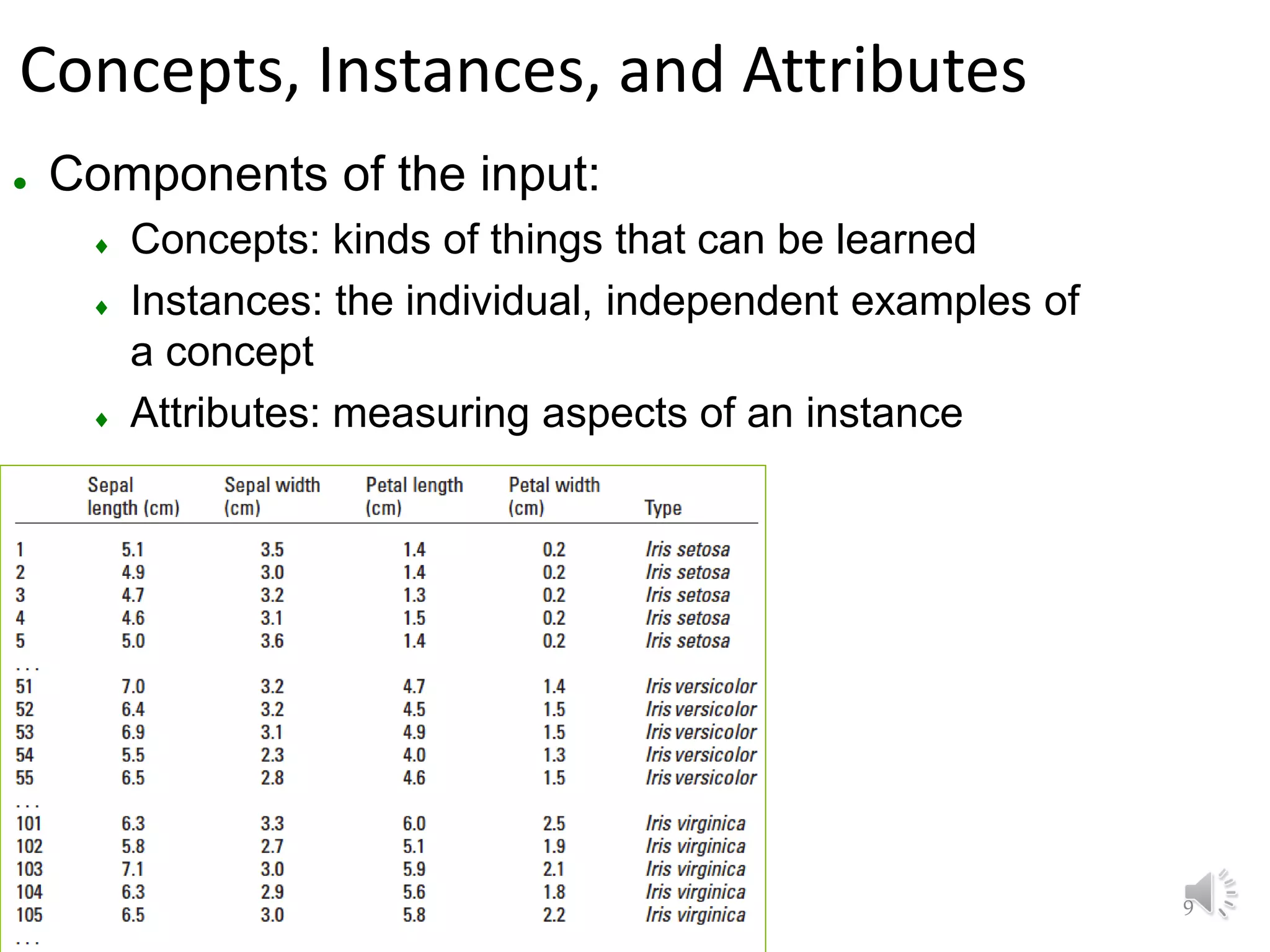
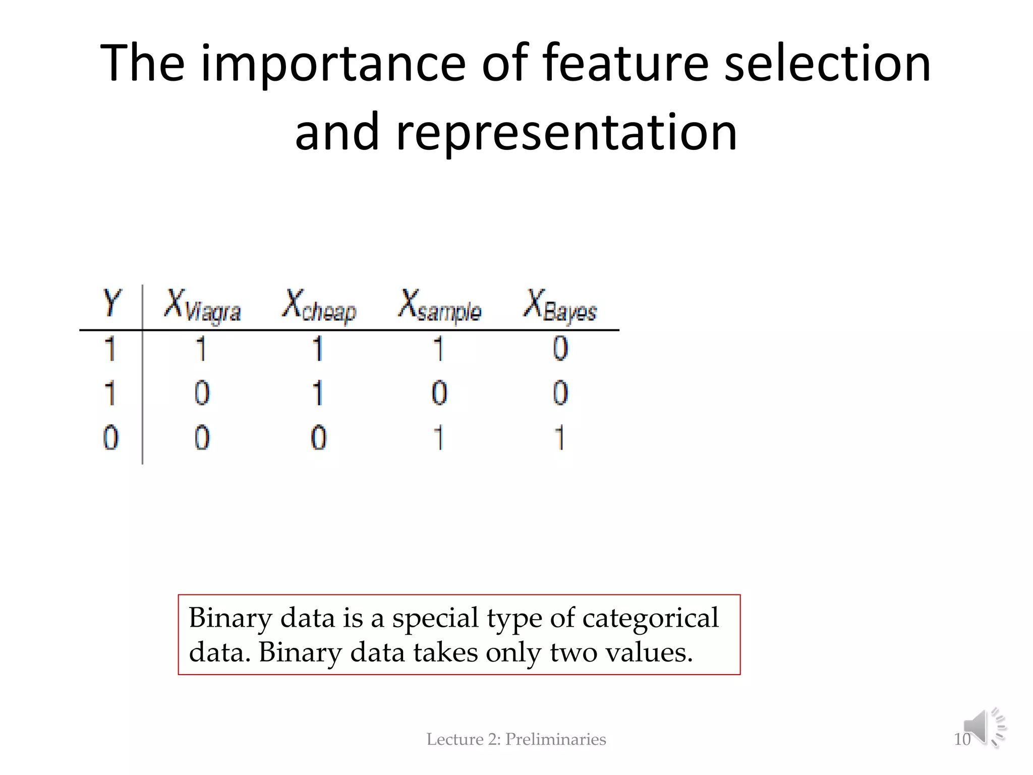
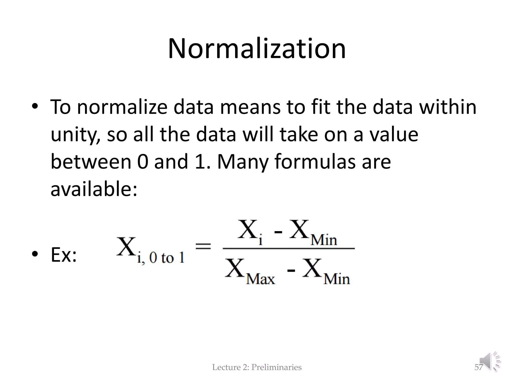
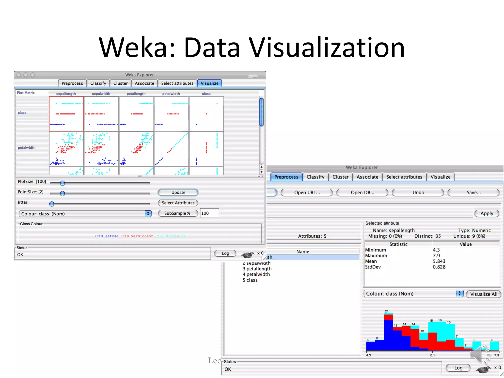


This document provides an overview of key concepts in machine learning and data preprocessing. It discusses raw data and feature representation, including concepts, instances, attributes, and features. It also includes digressions on statistics such as measures of central tendency, normalization, and data visualization techniques. The document is a lecture on preliminaries for machine learning and language technology.