Downloaded 245 times

![S, G, and the Version Space Lecture 2: Basic Concepts 19 most specific hypothesis, S most general hypothesis, G h H, between S and G is consistent [E( h | X) = 0] and make up the version space](https://image.slidesharecdn.com/lecture2basicconceptsofmachinelearning-140814084140-phpapp01/75/Lecture-2-Basic-Concepts-in-Machine-Learning-for-Language-Technology-19-2048.jpg)
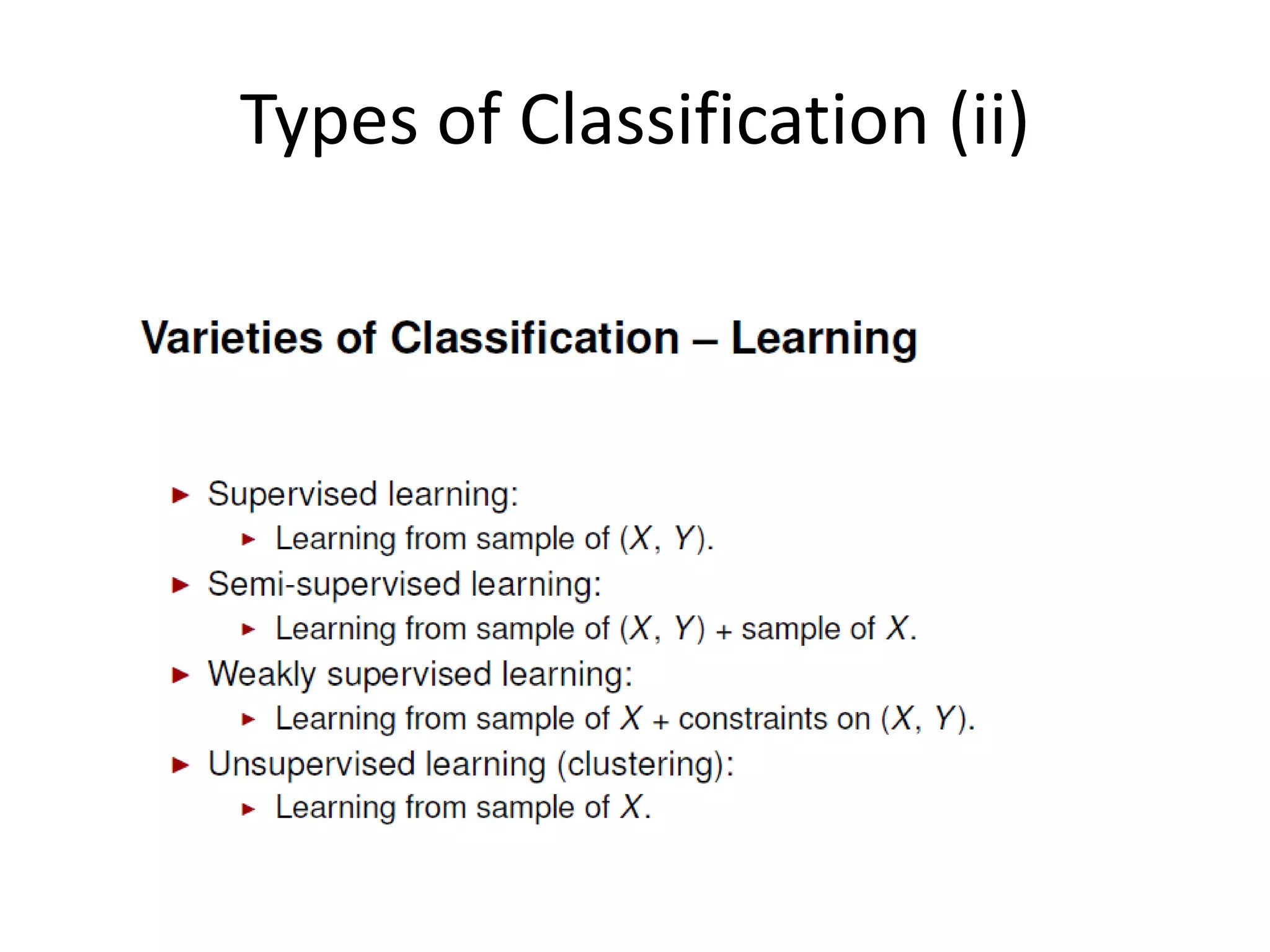

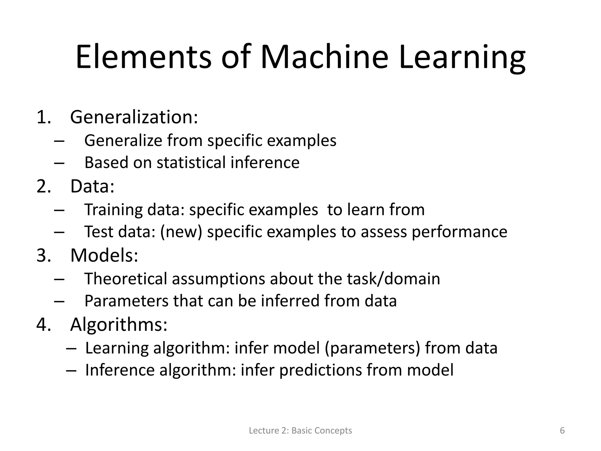
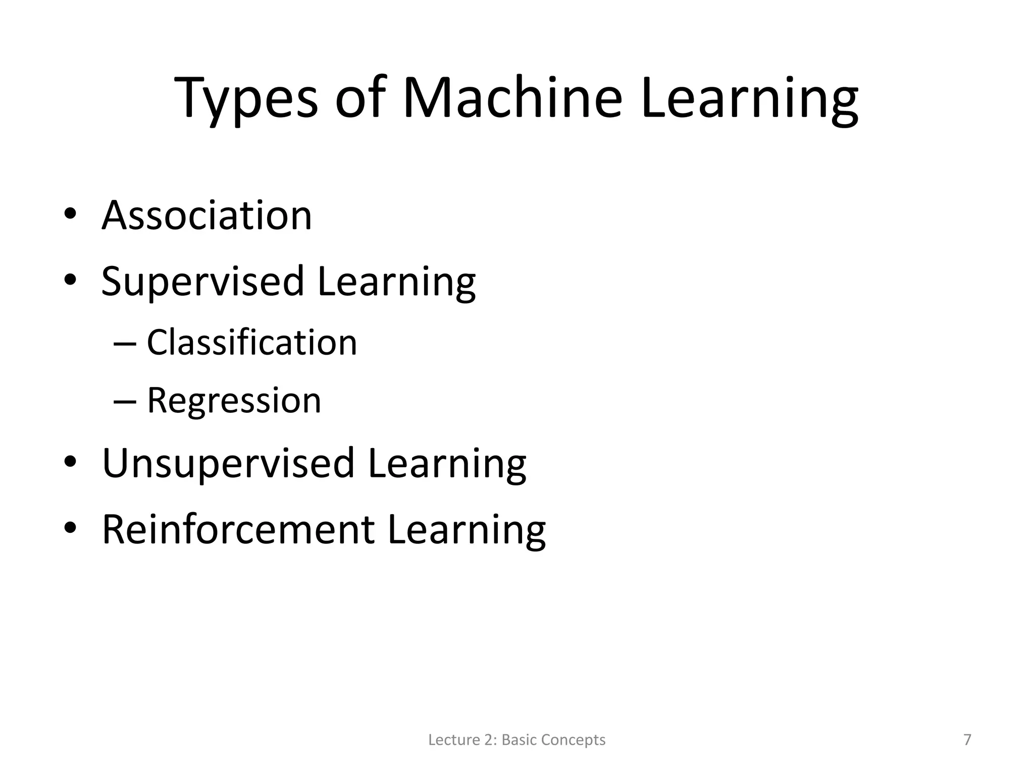
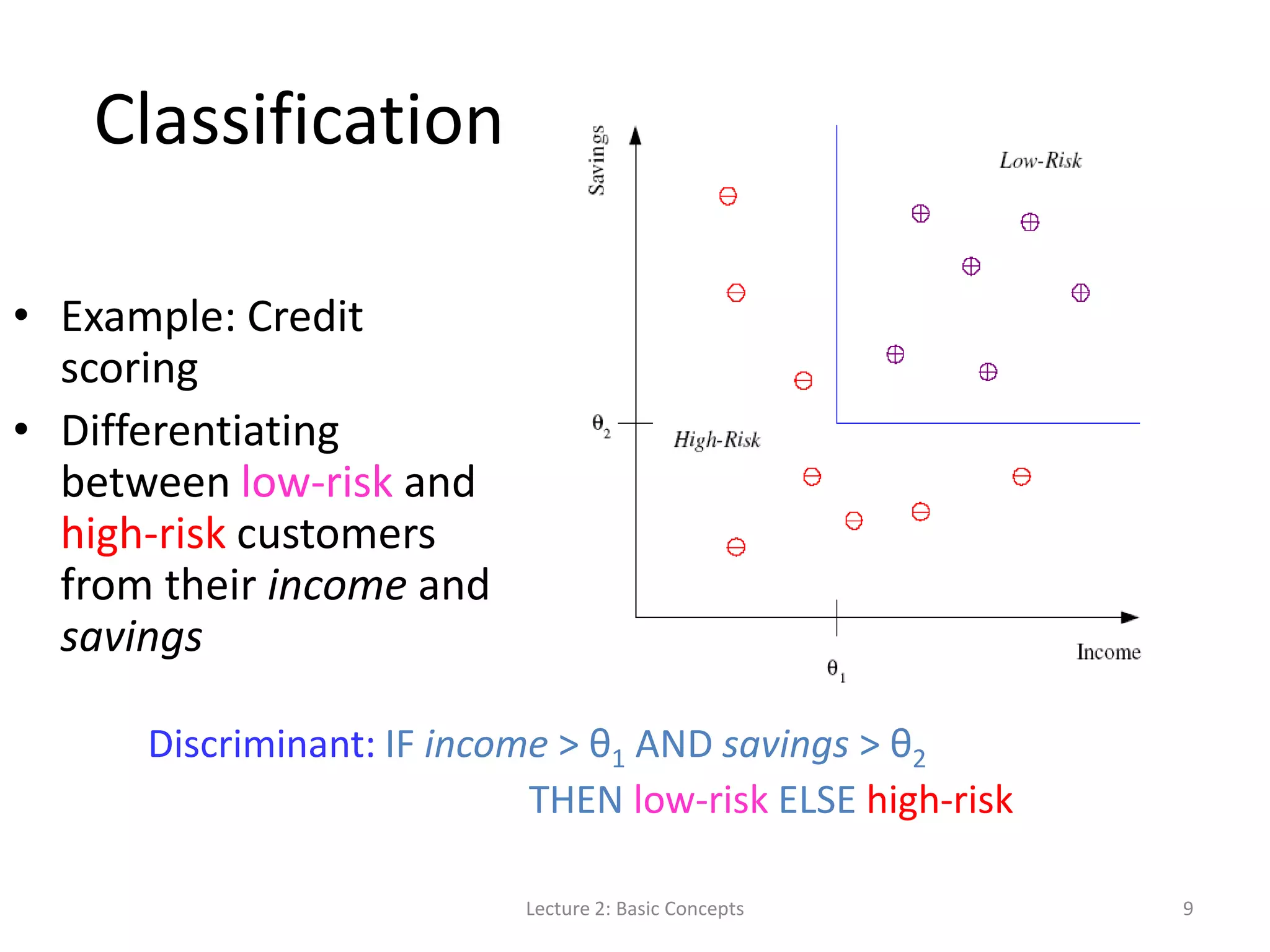
This document covers the basics of machine learning, including definitions, types (supervised, unsupervised, and reinforcement learning), and key concepts such as classification, regression, and generalization. It explains the elements of machine learning and the importance of training data, models, and algorithms, along with applications in natural language processing. Additionally, it discusses model selection, cross-validation, and assessing generalization error.