Know Your Data in data mining applications

DATA MINING Lecture 3: KnowYour Data Slides Adapted from Jiawei Han et al. and Jianlin Cheng DEPARTMENTOFCOMPUTER SCIENCE,UNIVERSITYOF COLORADO,COLORADO SPRINGS. CS4434/5434ANDDASE4435 DATAMINING, FALL2023 DR.OLUWATOSIN OLUWADARE,2023

2 Data Mining: Concepts and Techniques — Chapter 2 — Jiawei Han, Micheline Kamber, and Jian Pei University of Illinois at Urbana-Champaign Simon Fraser University ©2011 Han, Kamber, and Pei. All rights reserved.

3 Chapter 2: Getting to Know Your Data  Data Objects and Attribute Types  Basic Statistical Descriptions of Data  Data Visualization  Measuring Data Similarity and Dissimilarity  Summary

4 Types of Data Sets  Record  Relational records  Data matrix, e.g., numerical matrix, crosstabs  Document data: text documents: term- frequency vector  Transaction data  Graph and network  World Wide Web  Social or information networks  Molecular Structures  Ordered  Video data: sequence of images  Temporal data: time-series  Sequential Data: transaction sequences  Genetic sequence data  Spatial, image and multimedia:  Spatial data: maps  Image data:  Video data: Document 1 season timeout lost wi n game score ball pla y coach team Document 2 Document 3 3 0 5 0 2 6 0 2 0 2 0 0 7 0 2 1 0 0 3 0 0 1 0 0 1 2 2 0 3 0 TID Items 1 Bread, Coke, Milk 2 Beer, Bread 3 Beer, Coke, Diaper, Milk 4 Beer, Bread, Diaper, Milk 5 Coke, Diaper, Milk

5 Important Characteristics of Structured Data  Dimensionality  Curse of dimensionality  Sparsity  Only presence counts  Resolution  Patterns depend on the scale  Distribution  Centrality and dispersion

6 Data Objects  Data sets are made up of data objects.  A data object represents an entity.  Examples:  sales database: customers, store items, sales  medical database: patients, treatments  university database: students, professors, courses  Also called samples , examples, instances, data points, objects, tuples.  Data objects are described by attributes.  Database rows -> data objects; columns ->attributes.

7 Attributes  Attribute (or dimensions, features, variables): a data field, representing a characteristic or feature of a data object.  E.g., customer _ID, name, address  Types:  Nominal  Binary  Numeric: quantitative  Interval-scaled  Ratio-scaled

Data Attributes  Attribute refers to the characteristic of the data object.  The nouns defining the characteristics are used interchangeably: Attribute, dimension, feature, and variable. 8 Field Data Warehousing Database and Data Mining Statistic Machine Learning Characteristic term Used Feature Attribute Variable Dimension

9 Attribute Types  Nominal: categories, states, or “names of things”  Hair_color = {auburn, black, blond, brown, grey, red, white}  marital status, occupation, ID numbers, zip codes  Binary  Nominal attribute with only 2 states (0 and 1)  Symmetric binary: both outcomes equally important  e.g., cat or dog  Asymmetric binary: outcomes not equally important.  e.g., medical test (positive vs. negative)  Convention: assign 1 to most important outcome (e.g., HIV positive)  the positive (1) and negative (0) outcomes of a disease test.  Ordinal  Values have a meaningful order (ranking) but magnitude between successive values is not known.  Size = {small, medium, large}, grades, army rankings

10 Numeric Attribute Types  Quantity (integer or real-valued)  Interval  Measured on a scale of equal-sized units  Values have order  E.g., temperature in C˚or F˚, calendar dates  No true zero-point  Ratio  Inherent zero-point  We can speak of values as being an order of magnitude larger than the unit of measurement (10 K˚ is twice as high as 5 K˚).  e.g., temperature in Kelvin, length, counts, monetary quantities

11 Discrete vs. Continuous Attributes  Discrete Attribute  Has only a finite or countably infinite set of values  E.g., zip codes, profession, or the set of words in a collection of documents  Sometimes, represented as integer variables  Note: Binary attributes are a special case of discrete attributes  Continuous Attribute  Has real numbers as attribute values  E.g., temperature, height, or weight  Practically, real values can only be measured and represented using a finite number of digits  Continuous attributes are typically represented as floating-point variables

13 Basic Statistical Descriptions of Data  Motivation  To better understand the data: central tendency, variation and spread  Data dispersion characteristics  median, max, min, quantiles, outliers, variance, etc.  Numerical dimensions correspond to sorted intervals  Data dispersion: analyzed with multiple granularities of precision  Boxplot or quantile analysis on sorted intervals  Dispersion analysis on computed measures  Folding measures into numerical dimensions  Boxplot or quantile analysis on the transformed cube

14 Measuring the Central Tendency  Mean (algebraic measure) (sample vs. population): Note: n is sample size and N is population size.  Weighted arithmetic mean:  Trimmed mean: chopping extreme values  Median:  Middle value if odd number of values, or average of the middle two values otherwise  Estimated by interpolation (for grouped data):  Mode  Value that occurs most frequently in the data  Unimodal, bimodal, trimodal  Empirical formula:    n i i x n x 1 1      n i i n i i i w x w x 1 1 width freq l freq n L median median ) ) ( 2 / ( 1     ) ( 3 median mean mode mean     N x   

May 8, 2024 Data Mining: Concepts and Techniques 15 Symmetric vs. Skewed Data  Median, mean and mode of symmetric, positively and negatively skewed data positively skewed negatively skewed symmetric

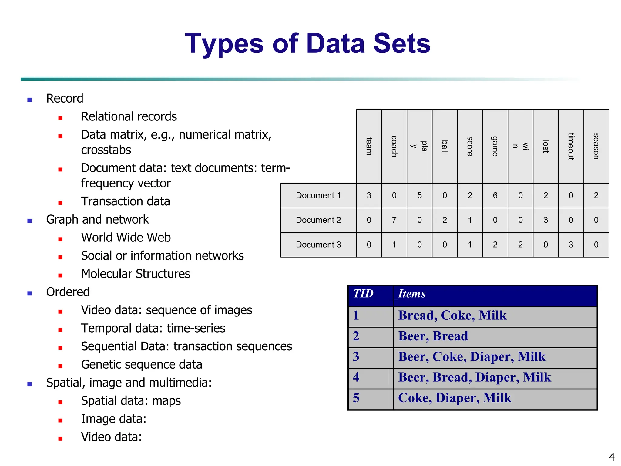
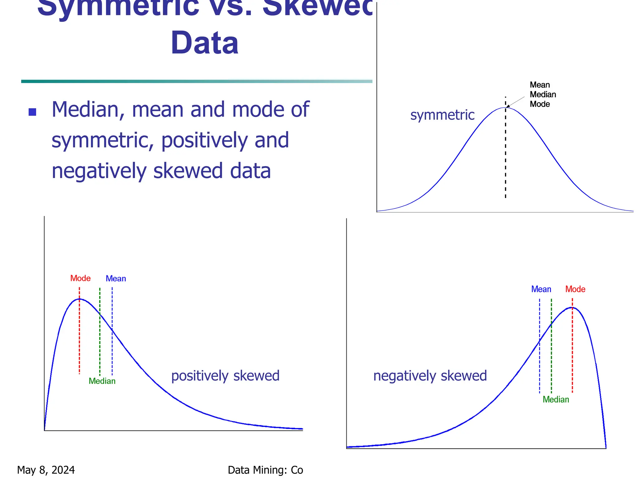
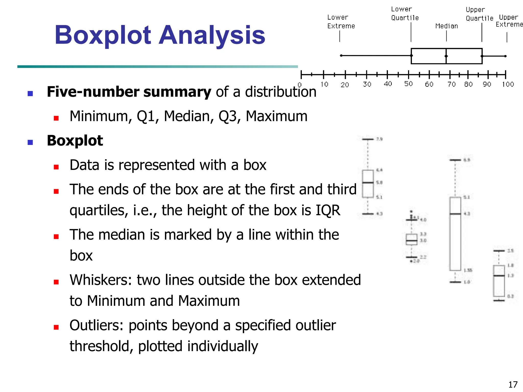
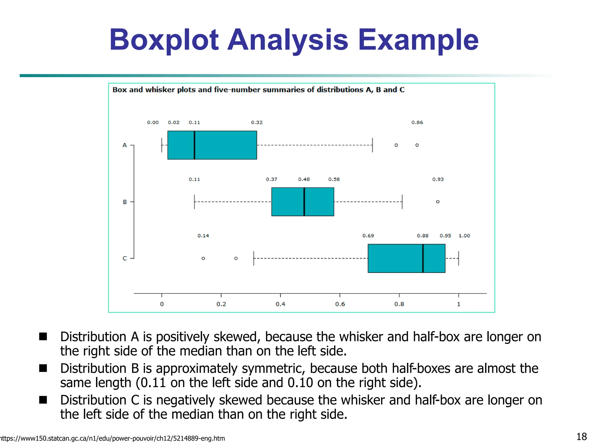
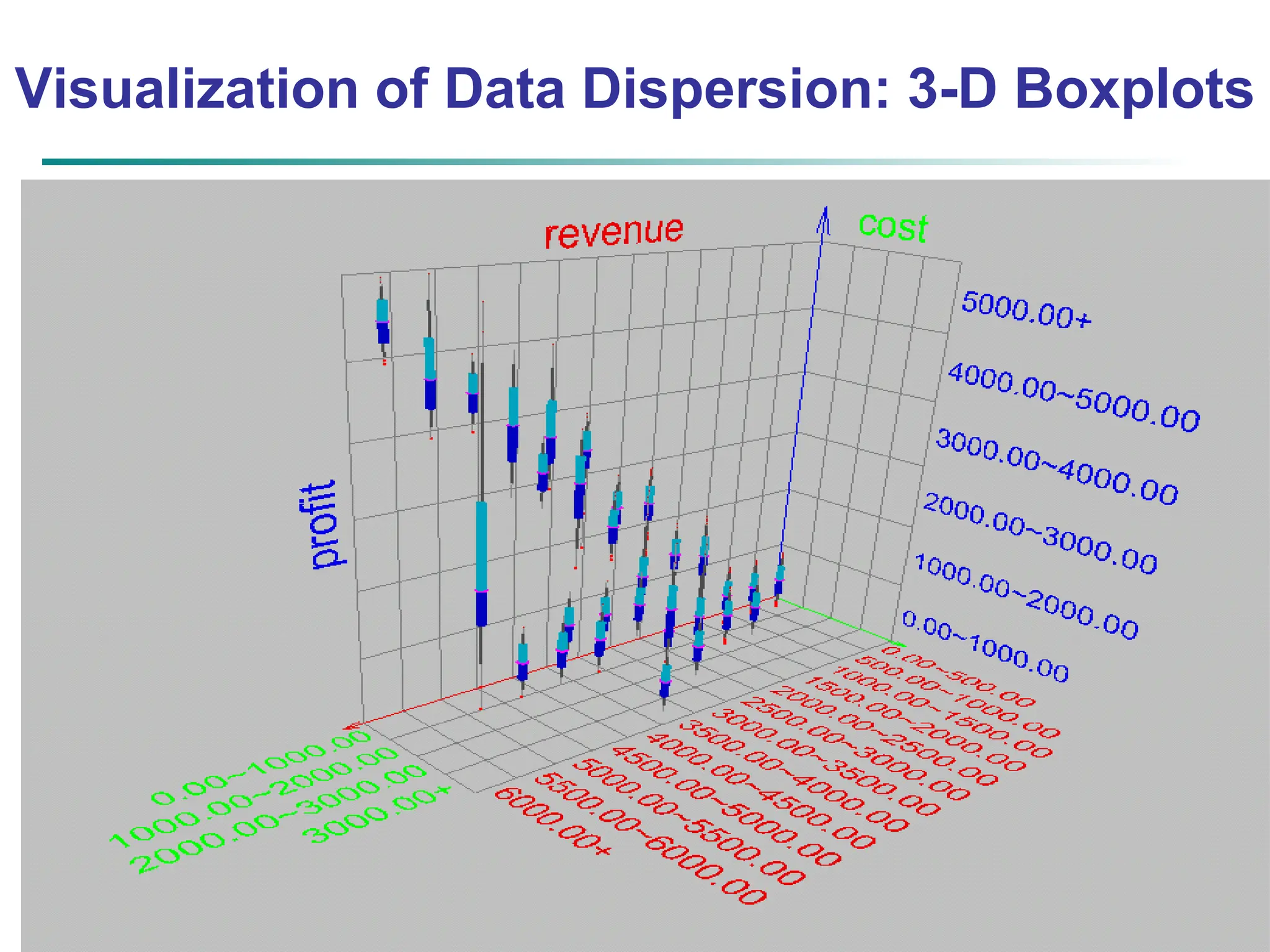
16 Measuring the Dispersion of Data  Quartiles, outliers and boxplots  Quartiles: Q1 (25th percentile), Q3 (75th percentile)  Inter-quartile range: IQR = Q3 – Q1  Five number summary: min, Q1, median, Q3, max  Boxplot: ends of the box are the quartiles; median is marked; add whiskers, and plot outliers individually  Outlier: usually, a value higher/lower than Q3 + 1.5 x IQR or Q1 – 1.5 x IQR  Variance and standard deviation (sample: s, population: σ)  Variance: (algebraic, scalable computation)  Standard deviation s (or σ) is the square root of variance s2 (or σ2)             n i n i i i n i i x n x n x x n s 1 1 2 2 1 2 2 ] ) ( 1 [ 1 1 ) ( 1 1         n i i n i i x N x N 1 2 2 1 2 2 1 ) ( 1   

17 Boxplot Analysis  Five-number summary of a distribution  Minimum, Q1, Median, Q3, Maximum  Boxplot  Data is represented with a box  The ends of the box are at the first and third quartiles, i.e., the height of the box is IQR  The median is marked by a line within the box  Whiskers: two lines outside the box extended to Minimum and Maximum  Outliers: points beyond a specified outlier threshold, plotted individually

Boxplot Analysis Example  Distribution A is positively skewed, because the whisker and half-box are longer on the right side of the median than on the left side.  Distribution B is approximately symmetric, because both half-boxes are almost the same length (0.11 on the left side and 0.10 on the right side).  Distribution C is negatively skewed because the whisker and half-box are longer on the left side of the median than on the right side. 18 https://www150.statcan.gc.ca/n1/edu/power-pouvoir/ch12/5214889-eng.htm

May 8, 2024 Data Mining: Concepts and Techniques 19 Visualization of Data Dispersion: 3-D Boxplots

20 Properties of Normal Distribution Curve  The normal (distribution) curve  From μ–σ to μ+σ: contains about 68% of the measurements (μ: mean, σ: standard deviation)  From μ–2σ to μ+2σ: contains about 95% of it  From μ–3σ to μ+3σ: contains about 99.7% of it

Standard deviation in a Normal Distribution 21 Images/google

22 Graphic Displays of Basic Statistical Descriptions  Boxplot: graphic display of five-number summary  Histogram: x-axis are values, y-axis repres. frequencies  Quantile plot: each value xi is paired with fi indicating that approximately 100 fi % of data are  xi  Quantile-quantile (q-q) plot: graphs the quantiles of one univariant distribution against the corresponding quantiles of another  Scatter plot: each pair of values is a pair of coordinates and plotted as points in the plane

23 Histogram Analysis  Histogram: Graph display of tabulated frequencies, shown as bars  It shows what proportion of cases fall into each of several categories  Differs from a bar chart in that it is the area of the bar that denotes the value, not the height as in bar charts, a crucial distinction when the categories are not of uniform width  The categories are usually specified as non-overlapping intervals of some variable. The categories (bars) must be adjacent 0 5 10 15 20 25 30 35 40 10000 30000 50000 70000 90000

Homework 1  Homework 1 has been posted at the course web site and on Canvas.  Due Sept. 12, 2023  Submit it to Canvas May 8, 2024 Data Mining: Concepts and Techniques 24

25 Histograms Often Tell More than Boxplots  The two histograms shown in the left may have the same boxplot representation  The same values for: min, Q1, median, Q3, max  But they have rather different data distributions

Data Mining: Concepts and Techniques 26 Quantile Plot  Displays all of the data (allowing the user to assess both the overall behavior and unusual occurrences)  Plots quantile information  For a data xi data sorted in increasing order, fi indicates that approximately 100 fi% of the data are below or equal to the value xi

27 Quantile-Quantile (Q-Q) Plot  Graphs the quantiles of one univariate distribution against the corresponding quantiles of another  View: Is there is a shift in going from one distribution to another?  Example shows unit price of items sold at Branch 1 vs. Branch 2 for each quantile. Unit prices of items sold at Branch 1 tend to be lower than those at Branch 2.

28 Scatter plot  Provides a first look at bivariate data to see clusters of points, outliers, etc  Each pair of values is treated as a pair of coordinates and plotted as points in the plane

29 Positively and Negatively Correlated Data  The left half fragment is positively correlated  The right half is negative correlated

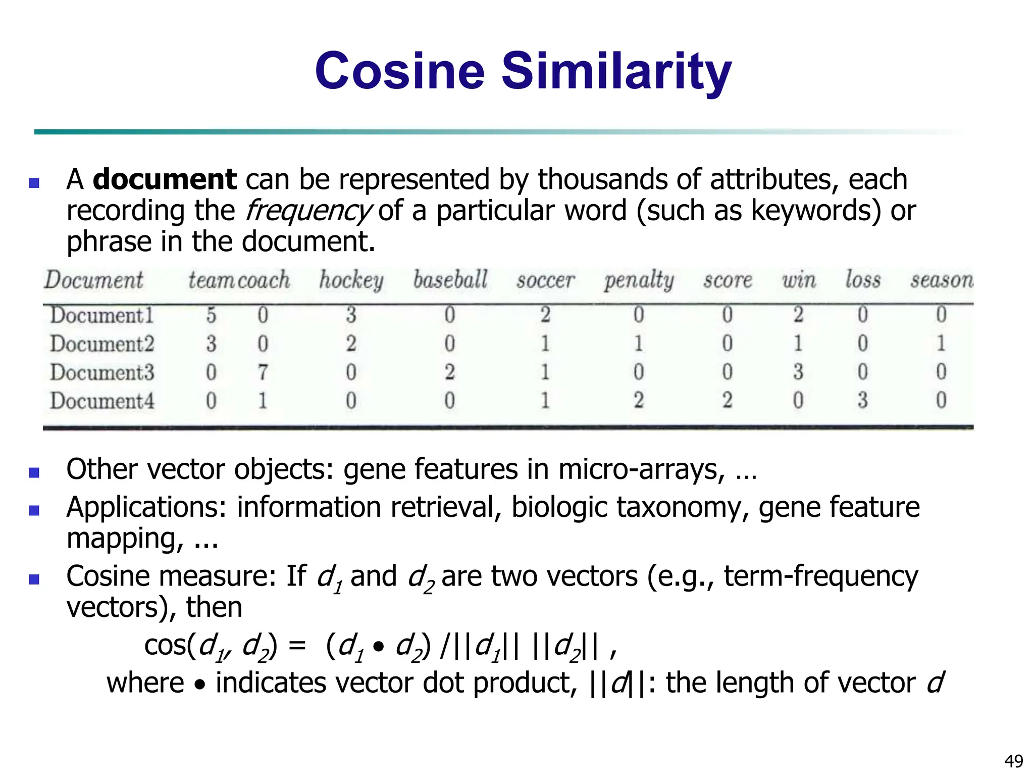
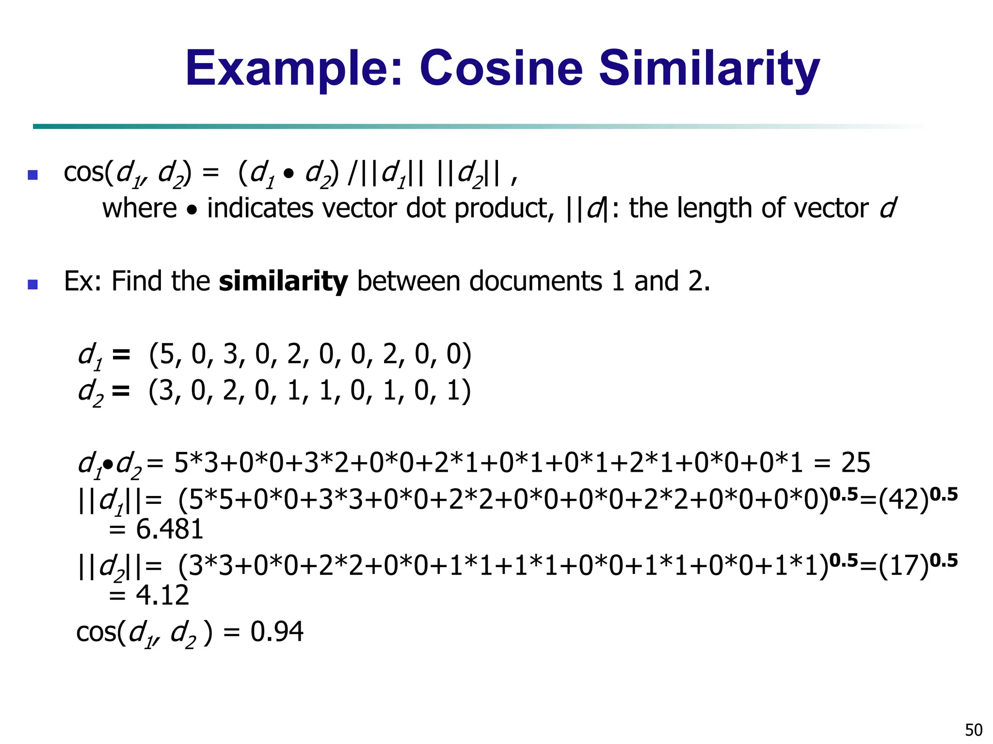
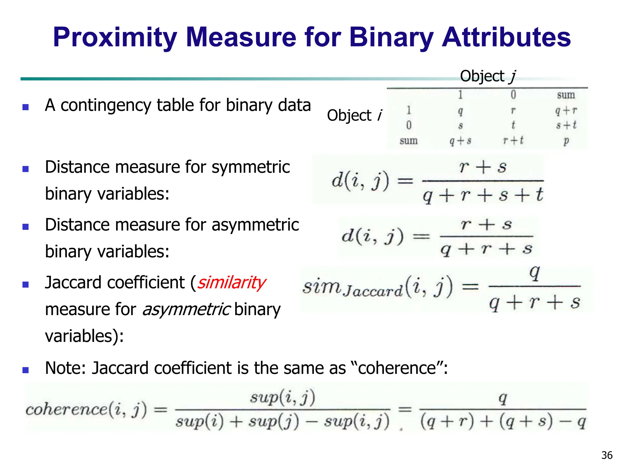
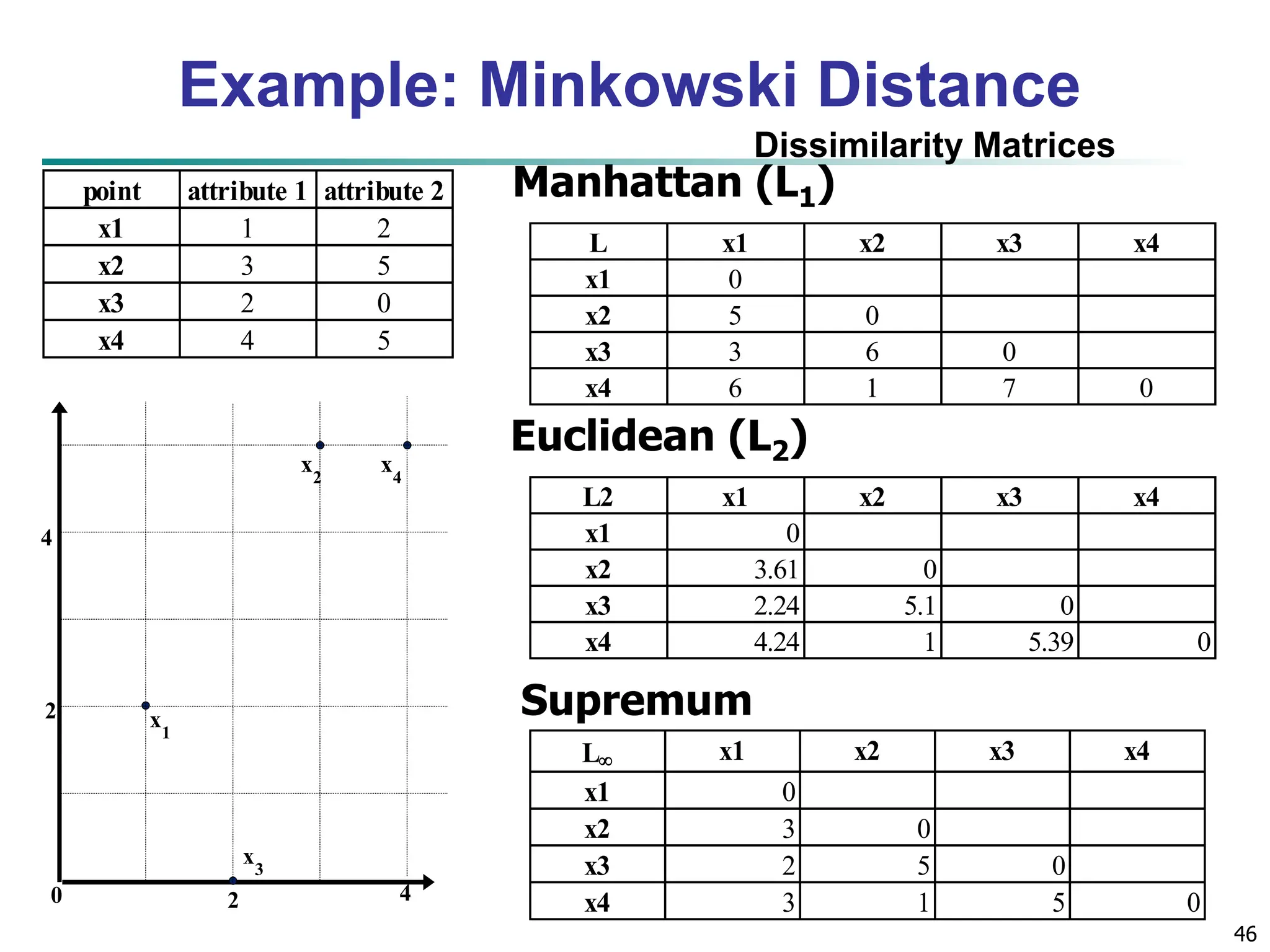
32 Similarity and Dissimilarity  Similarity  Numerical measure of how alike two data objects are  Value is higher when objects are more alike  Often falls in the range [0,1]  Dissimilarity (e.g., distance)  Numerical measure of how different two data objects are  Lower when objects are more alike  Minimum dissimilarity is often 0  Upper limit varies  Proximity refers to a similarity or dissimilarity

33 Data Matrix and Dissimilarity Matrix  Data matrix  n data points with p dimensions  Two modes  Dissimilarity matrix  n data points, but registers only the distance  A triangular matrix  Single mode                   np x ... nf x ... n1 x ... ... ... ... ... ip x ... if x ... i1 x ... ... ... ... ... 1p x ... 1f x ... 11 x                 0 ... ) 2 , ( ) 1 , ( : : : ) 2 , 3 ( ) ... n d n d 0 d d(3,1 0 d(2,1) 0

34 Proximity Measure for Nominal Attributes  Can take 2 or more states, e.g., red, yellow, blue, green (generalization of a binary attribute)  Method 1: Simple matching  m: # of matches, p: total # of variables  Method 2: Use a large number of binary attributes  creating a new binary attribute for each of the M nominal states p m p j i d   ) , (

Class Example: Method 1 35                 0 ... ) 2 , ( ) 1 , ( : : : ) 2 , 3 ( ) ... n d n d 0 d d(3,1 0 d(2,1) 0 p m p j i d   ) , (

36 Proximity Measure for Binary Attributes  A contingency table for binary data  Distance measure for symmetric binary variables:  Distance measure for asymmetric binary variables:  Jaccard coefficient (similarity measure for asymmetric binary variables):  Note: Jaccard coefficient is the same as “coherence”: Object i Object j

Variables (q, r, s ,t)  q is the number of attributes that equal 1 for both objects i and j,  r is the number of attributes that equal 1 for object i but equal 0 for object j,  s is the number of attributes that equal 0 for object i but equal 1 for object j, and  t is the number of attributes that equal 0 for both objects i and j. 37

38 Dissimilarity between Binary Variables  Example  Gender is a symmetric attribute  The remaining attributes are asymmetric binary attributes  Let the values Y(yes) and P(positive) be 1, and the value N(no and negative) 0 Name Gender Fever Cough Test-1 Test-2 Test-3 Test-4 Jack M Y N P N N N Mary F Y N P N P N Jim M Y P N N N N

Calculate the Dissimilarity  d(Jack, Mary) = ?  d(Jack, Jim). = ?  d(Jim, Jack) = ?  q is the number of attributes that equal 1 for both objects i and j,  r is the number of attributes that equal 1 for object i but equal 0 for object j,  s is the number of attributes that equal 0 for object i but equal 1 for object j, and  t is the number of attributes that equal 0 for both objects i and j. 39 OR

40 Dissimilarity between Binary Variables  Example  Gender is a symmetric attribute  The remaining attributes are asymmetric binary attributes  Let the values Y(yes) and P(positive) be 1, and the value N(no and negative) 0 Name Gender Fever Cough Test-1 Test-2 Test-3 Test-4 Jack M Y N P N N N Mary F Y N P N P N Jim M Y P N N N N 75 . 0 2 1 1 2 1 ) , ( 67 . 0 1 1 1 1 1 ) , ( 33 . 0 1 0 2 1 0 ) , (                mary jim d jim jack d mary jack d

Comment on the Result  What does the measurement suggest?  These measurements suggest that Jim and Mary are unlikely to have a similar disease because they have the highest dissimilarity value among the three pairs.  Of the three patients, Jack and Mary are the most likely to have a similar disease. 41

42 Standardizing Numeric Data  Z-score:  X: raw score to be standardized, μ: mean of the population, σ: standard deviation  the distance between the raw score and the population mean in units of the standard deviation  negative when the raw score is below the mean, “+” when above  An alternative way: Calculate the mean absolute deviation where  standardized measure (z-score):  Using mean absolute deviation is more robust than using standard deviation . ) ... 2 1 1 nf f f f x x (x n m     |) | ... | | | (| 1 2 1 f nf f f f f f m x m x m x n s        f f if if s m x z       x z

43 Example: Data Matrix and Dissimilarity Matrix point attribute1 attribute2 x1 1 2 x2 3 5 x3 2 0 x4 4 5 Dissimilarity Matrix (with Euclidean Distance) x1 x2 x3 x4 x1 0 x2 3.61 0 x3 5.1 5.1 0 x4 4.24 1 5.39 0 Data Matrix

44 Distance on Numeric Data: Minkowski Distance  Minkowski distance: A popular distance measure where i = (xi1, xi2, …, xip) and j = (xj1, xj2, …, xjp) are two p-dimensional data objects, and h is the order (the distance so defined is also called L-h norm)  Properties  d(i, j) > 0 if i ≠ j, and d(i, i) = 0 (Positive definiteness)  d(i, j) = d(j, i) (Symmetry)  d(i, j)  d(i, k) + d(k, j) (Triangle Inequality)  A distance that satisfies these properties is a metric

45 Special Cases of Minkowski Distance  h = 1: Manhattan (city block, L1 norm) distance  E.g., the Hamming distance: the number of bits that are different between two binary vectors  h = 2: (L2 norm) Euclidean distance  h  . “supremum” (Lmax norm, L norm) distance.  This is the maximum difference between any component (attribute) of the vectors ) | | ... | | | (| ) , ( 2 2 2 2 2 1 1 p p j x i x j x i x j x i x j i d        | | ... | | | | ) , ( 2 2 1 1 p p j x i x j x i x j x i x j i d       

46 Example: Minkowski Distance Dissimilarity Matrices point attribute 1 attribute 2 x1 1 2 x2 3 5 x3 2 0 x4 4 5 L x1 x2 x3 x4 x1 0 x2 5 0 x3 3 6 0 x4 6 1 7 0 L2 x1 x2 x3 x4 x1 0 x2 3.61 0 x3 2.24 5.1 0 x4 4.24 1 5.39 0 L x1 x2 x3 x4 x1 0 x2 3 0 x3 2 5 0 x4 3 1 5 0 Manhattan (L1) Euclidean (L2) Supremum

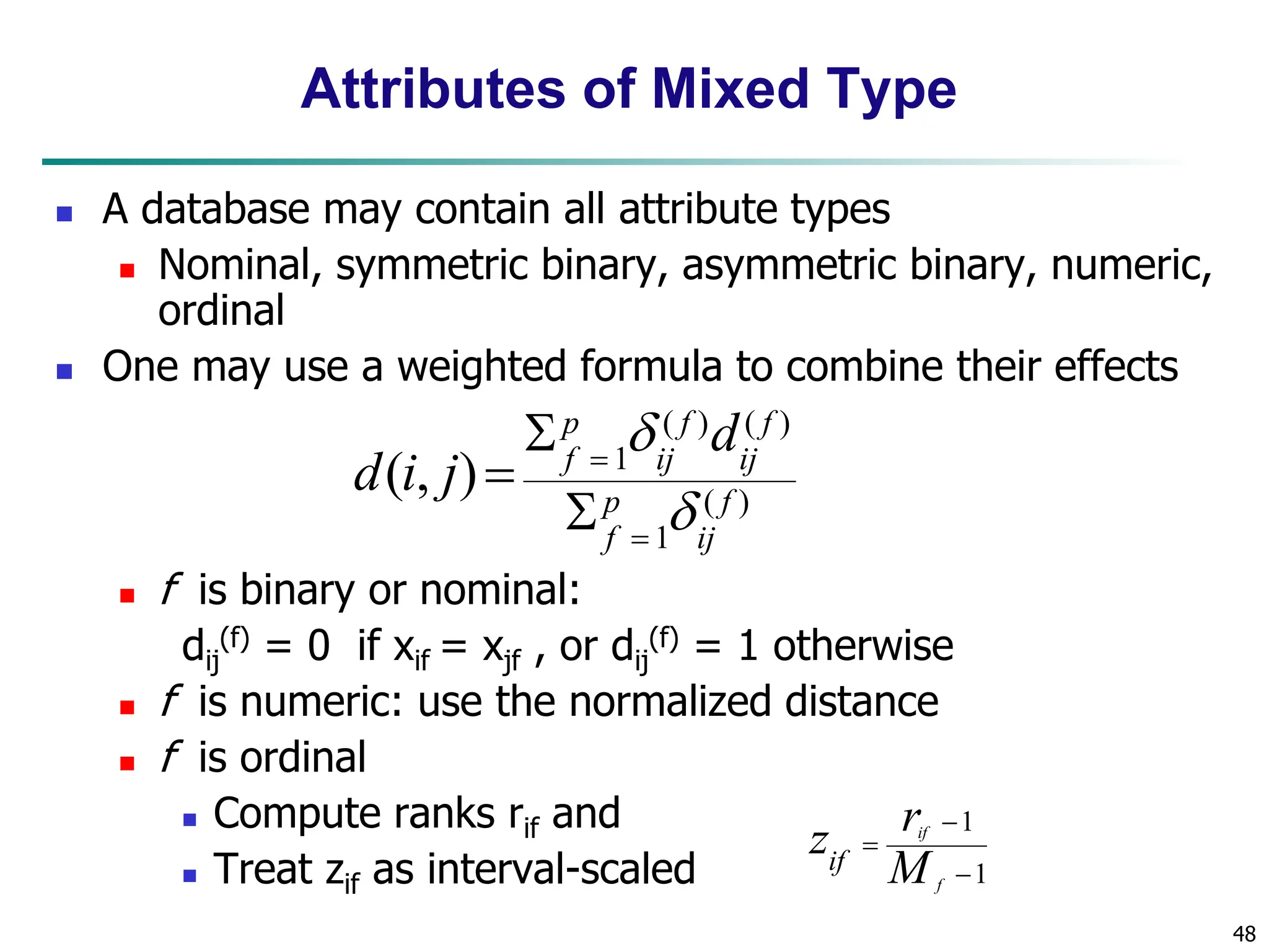
47 Ordinal Variables  An ordinal variable can be discrete or continuous  Order is important, e.g., rank  Can be treated like interval-scaled  replace xif by their rank  map the range of each variable onto [0, 1] by replacing i-th object in the f-th variable by  compute the dissimilarity using methods for interval- scaled variables 1 1    f if if M r z } ,..., 1 { f if M r 

48 Attributes of Mixed Type  A database may contain all attribute types  Nominal, symmetric binary, asymmetric binary, numeric, ordinal  One may use a weighted formula to combine their effects  f is binary or nominal: dij (f) = 0 if xif = xjf , or dij (f) = 1 otherwise  f is numeric: use the normalized distance  f is ordinal  Compute ranks rif and  Treat zif as interval-scaled ) ( 1 ) ( ) ( 1 ) , ( f ij p f f ij f ij p f d j i d        1 1    f if M r zif

49 Cosine Similarity  A document can be represented by thousands of attributes, each recording the frequency of a particular word (such as keywords) or phrase in the document.  Other vector objects: gene features in micro-arrays, …  Applications: information retrieval, biologic taxonomy, gene feature mapping, ...  Cosine measure: If d1 and d2 are two vectors (e.g., term-frequency vectors), then cos(d1, d2) = (d1  d2) /||d1|| ||d2|| , where  indicates vector dot product, ||d||: the length of vector d

50 Example: Cosine Similarity  cos(d1, d2) = (d1  d2) /||d1|| ||d2|| , where  indicates vector dot product, ||d|: the length of vector d  Ex: Find the similarity between documents 1 and 2. d1 = (5, 0, 3, 0, 2, 0, 0, 2, 0, 0) d2 = (3, 0, 2, 0, 1, 1, 0, 1, 0, 1) d1d2 = 5*3+0*0+3*2+0*0+2*1+0*1+0*1+2*1+0*0+0*1 = 25 ||d1||= (5*5+0*0+3*3+0*0+2*2+0*0+0*0+2*2+0*0+0*0)0.5=(42)0.5 = 6.481 ||d2||= (3*3+0*0+2*2+0*0+1*1+1*1+0*0+1*1+0*0+1*1)0.5=(17)0.5 = 4.12 cos(d1, d2 ) = 0.94

Summary  Data attribute types: nominal, binary, ordinal, interval-scaled, ratio- scaled  Many types of data sets, e.g., numerical, text, graph, Web, image.  Gain insight into the data by:  Basic statistical data description: central tendency, dispersion, graphical displays  Data visualization: map data onto graphical primitives  Measure data similarity  Above steps are the beginning of data preprocessing.  Many methods have been developed but still an active area of research. 52

References  W. Cleveland, Visualizing Data, Hobart Press, 1993  T. Dasu and T. Johnson. Exploratory Data Mining and Data Cleaning. John Wiley, 2003  U. Fayyad, G. Grinstein, and A. Wierse. Information Visualization in Data Mining and Knowledge Discovery, Morgan Kaufmann, 2001  L. Kaufman and P. J. Rousseeuw. Finding Groups in Data: an Introduction to Cluster Analysis. John Wiley & Sons, 1990.  H. V. Jagadish, et al., Special Issue on Data Reduction Techniques. Bulletin of the Tech. Committee on Data Eng., 20(4), Dec. 1997  D. A. Keim. Information visualization and visual data mining, IEEE trans. on Visualization and Computer Graphics, 8(1), 2002  D. Pyle. Data Preparation for Data Mining. Morgan Kaufmann, 1999  S. Santini and R. Jain,” Similarity measures”, IEEE Trans. on Pattern Analysis and Machine Intelligence, 21(9), 1999  E. R. Tufte. The Visual Display of Quantitative Information, 2nd ed., Graphics Press, 2001  C. Yu , et al., Visual data mining of multimedia data for social and behavioral studies, Information Visualization, 8(1), 2009 53

Know Your Data in data mining applications

More Related Content

Similar to Know Your Data in data mining applications

Recently uploaded

Know Your Data in data mining applications