2 Chapter 2: Gettingto Know Your Data Data Objects and Attribute Types Basic Statistical Descriptions of Data Data Visualization Measuring Data Similarity and Dissimilarity Summary
3.
3 Types of DataSets Record Relational records Data matrix, e.g., numerical matrix, crosstabs Document data: text documents: term- frequency vector Transaction data Graph and network World Wide Web Social or information networks Molecular Structures Ordered Video data: sequence of images Temporal data: time-series Sequential Data: transaction sequences Genetic sequence data Spatial, image and multimedia: Spatial data: maps Image data: Video data: Document 1 season timeout lost wi n game score ball pla y coach team Document 2 Document 3 3 0 5 0 2 6 0 2 0 2 0 0 7 0 2 1 0 0 3 0 0 1 0 0 1 2 2 0 3 0 TID Items 1 Bread, Coke, Milk 2 Beer, Bread 3 Beer, Coke, Diaper, Milk 4 Beer, Bread, Diaper, Milk 5 Coke, Diaper, Milk
4.
4 Data Objects Datasets are made up of data objects. A data object represents an entity. Examples: sales database: customers, store items, sales medical database: patients, treatments university database: students, professors, courses Also called samples , examples, instances, data points, objects, tuples. Data objects are described by attributes. Database rows -> data objects; columns ->attributes.
5.
5 Attributes Attribute (ordimensions, features, variables): a data field, representing a characteristic or feature of a data object. E.g., customer _ID, name, address Types: Nominal Binary Numeric: quantitative Interval-scaled Ratio-scaled
6.
6 Attribute Types Nominal:Nominal means “relating to names.” The values of a nominal attribute are symbols or names of things. Each value represents some kind of category, code, or state. nominal attribute values do not have any meaningful order about them and are not quantitative. Hair_color = {black, blond, brown, grey, red, white} marital status, occupation, ID numbers, zip codes Binary Nominal attribute with only 2 states (0 and 1) 0 typically means that the attribute is absent, 1 means present Example: attribute smoker describing a patient Symmetric binary: both outcomes equally important e.g., gender Asymmetric binary: outcomes not equally important. e.g., medical test (positive vs. negative) Ordinal Values have a meaningful order or ranking among them but magnitude between successive values is not known. Size = {small, medium, large}, grades, army rankings
7.
Quantity (integeror real-valued) Interval Measured on a scale of equal-sized units Values have order E.g., temperature in C˚or F˚, calendar dates Quantify the difference between values. For example, temperature of 20◦C is five degrees higher than a temperature of 15◦C. Calendar dates - the years 2002 and 2010 are eight years apart. No true zero-point - neither 0◦C nor 0◦F indicates “no temperature.” Ratio Inherent zero-point, value as being a multiple (or ratio) of another We can speak of values as being an order of magnitude larger than the unit of measurement (10 K˚ is twice as high as 5 K˚). e.g., temperature in Kelvin, length, counts, monetary quantities 7 Numeric Attribute Types
8.
8 Discrete vs. ContinuousAttributes Discrete Attribute Has only a finite or countably infinite set of values E.g., zip codes, profession, or the set of words in a collection of documents Sometimes, represented as integer variables Note: Binary attributes are a special case of discrete attributes Continuous Attribute Has real numbers as attribute values E.g., temperature, height, or weight Practically, real values can only be measured and represented using a finite number of digits Continuous attributes are typically represented as floating-point variables
9.
9 Chapter 2: Gettingto Know Your Data Data Objects and Attribute Types Basic Statistical Descriptions of Data Data Visualization Measuring Data Similarity and Dissimilarity Summary
10.
10 Basic Statistical Descriptionsof Data Motivation To better understand the data: central tendency, variation and spread Data dispersion characteristics median, max, min, quantiles, outliers, variance, etc. Numerical dimensions correspond to sorted intervals Data dispersion: analyzed with multiple granularities of precision Boxplot or quantile analysis on sorted intervals Dispersion analysis on computed measures Folding measures into numerical dimensions Boxplot or quantile analysis on the transformed cube
11.
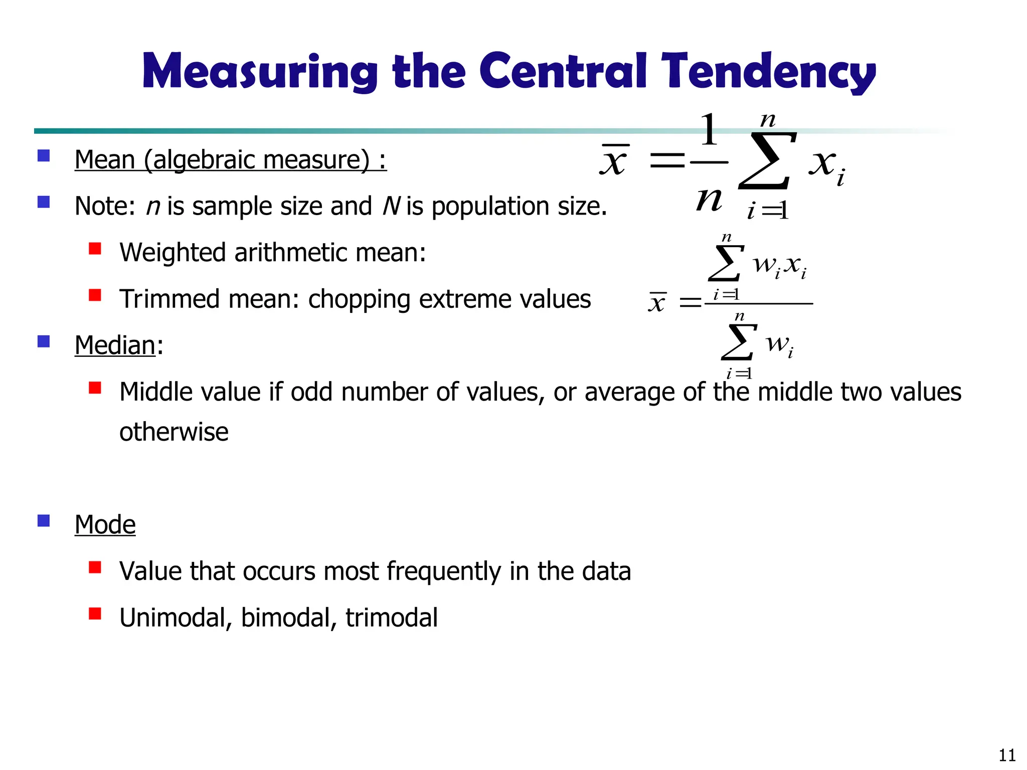
11 Measuring the CentralTendency Mean (algebraic measure) : Note: n is sample size and N is population size. Weighted arithmetic mean: Trimmed mean: chopping extreme values Median: Middle value if odd number of values, or average of the middle two values otherwise Mode Value that occurs most frequently in the data Unimodal, bimodal, trimodal n i i x n x 1 1 n i i n i i i w x w x 1 1
12.
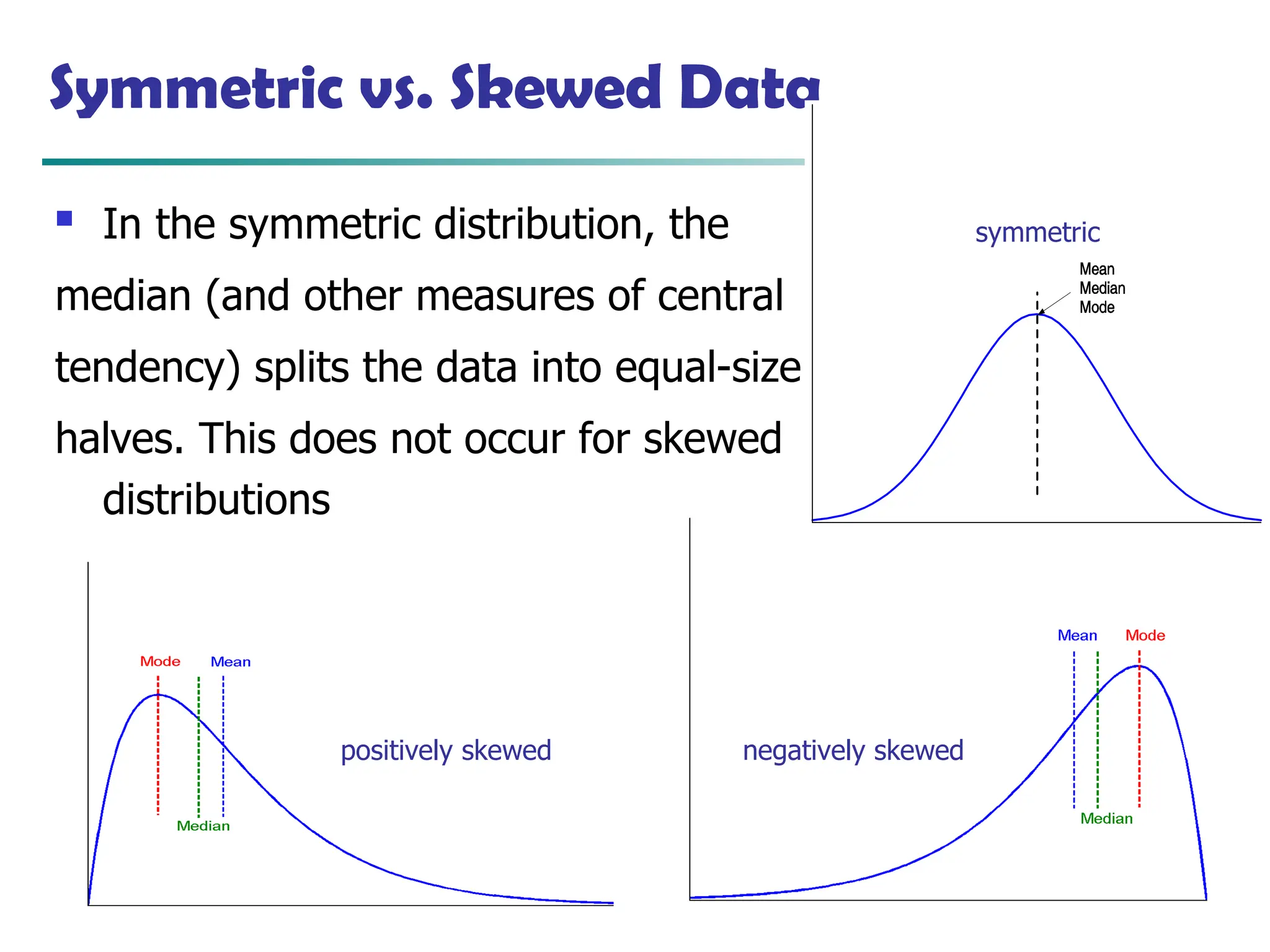
March 5, 2025Data Mining: Concepts and Techniques In the symmetric distribution, the median (and other measures of central tendency) splits the data into equal-size halves. This does not occur for skewed distributions 12 Symmetric vs. Skewed Data positively skewed negatively skewed symmetric
13.
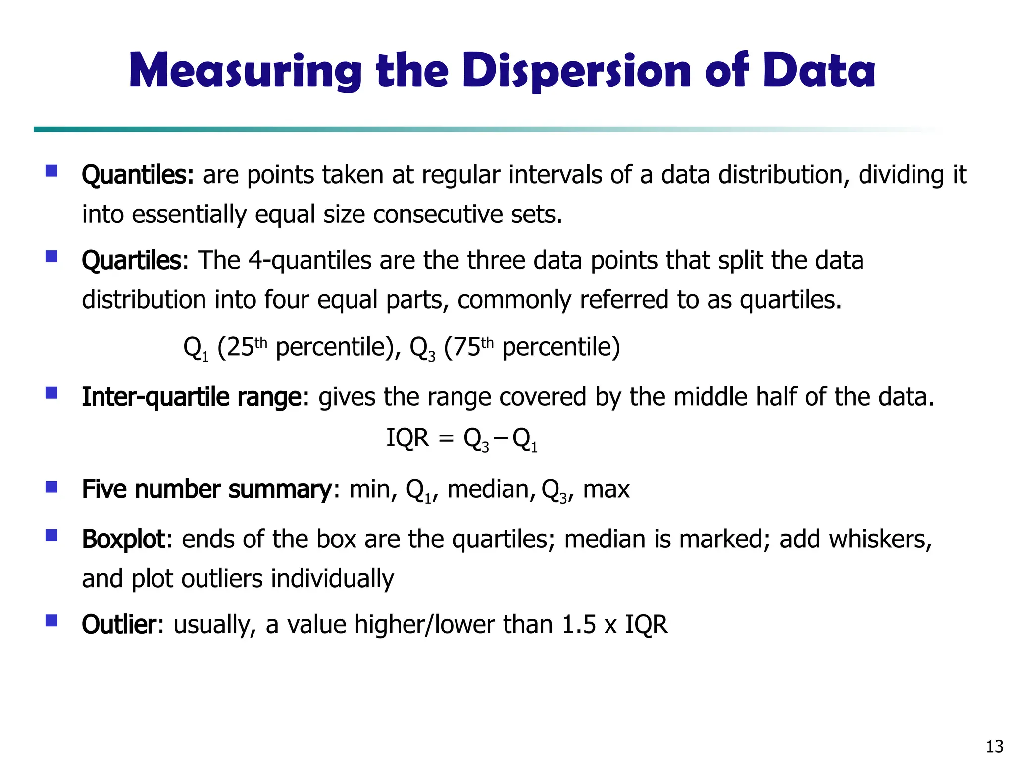
13 Measuring the Dispersionof Data Quantiles: are points taken at regular intervals of a data distribution, dividing it into essentially equal size consecutive sets. Quartiles: The 4-quantiles are the three data points that split the data distribution into four equal parts, commonly referred to as quartiles. Q1 (25th percentile), Q3 (75th percentile) Inter-quartile range: gives the range covered by the middle half of the data. IQR = Q3 – Q1 Five number summary: min, Q1, median, Q3, max Boxplot: ends of the box are the quartiles; median is marked; add whiskers, and plot outliers individually Outlier: usually, a value higher/lower than 1.5 x IQR
14.
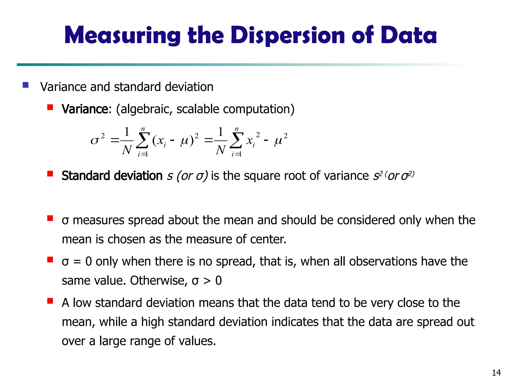
14 Measuring the Dispersionof Data Variance and standard deviation Variance: (algebraic, scalable computation) Standard deviation s (or σ) is the square root of variance s2 (or σ2) σ measures spread about the mean and should be considered only when the mean is chosen as the measure of center. σ = 0 only when there is no spread, that is, when all observations have the same value. Otherwise, σ > 0 A low standard deviation means that the data tend to be very close to the mean, while a high standard deviation indicates that the data are spread out over a large range of values. n i i n i i x N x N 1 2 2 1 2 2 1 ) ( 1
15.
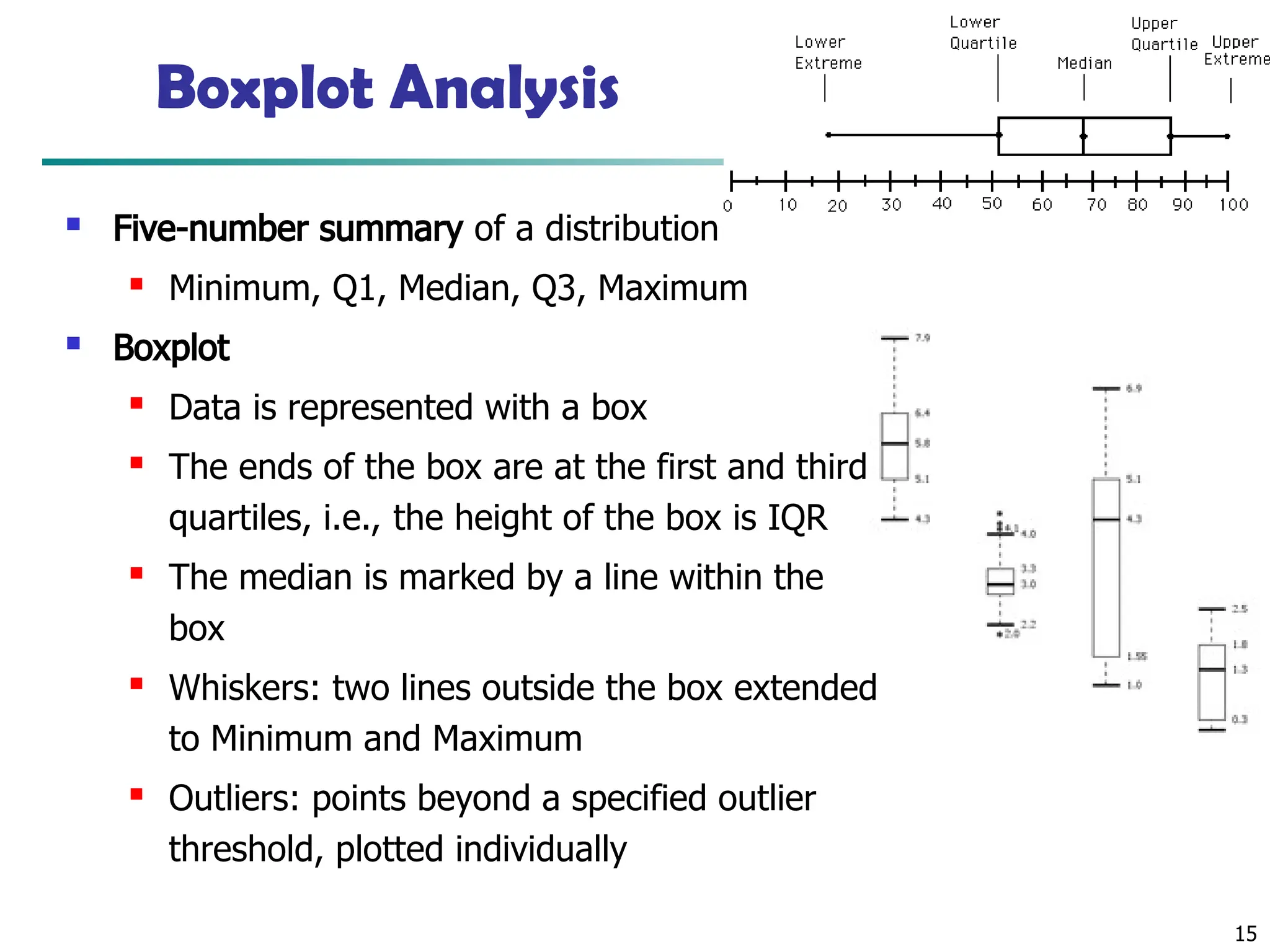
15 Boxplot Analysis Five-numbersummary of a distribution Minimum, Q1, Median, Q3, Maximum Boxplot Data is represented with a box The ends of the box are at the first and third quartiles, i.e., the height of the box is IQR The median is marked by a line within the box Whiskers: two lines outside the box extended to Minimum and Maximum Outliers: points beyond a specified outlier threshold, plotted individually
16.
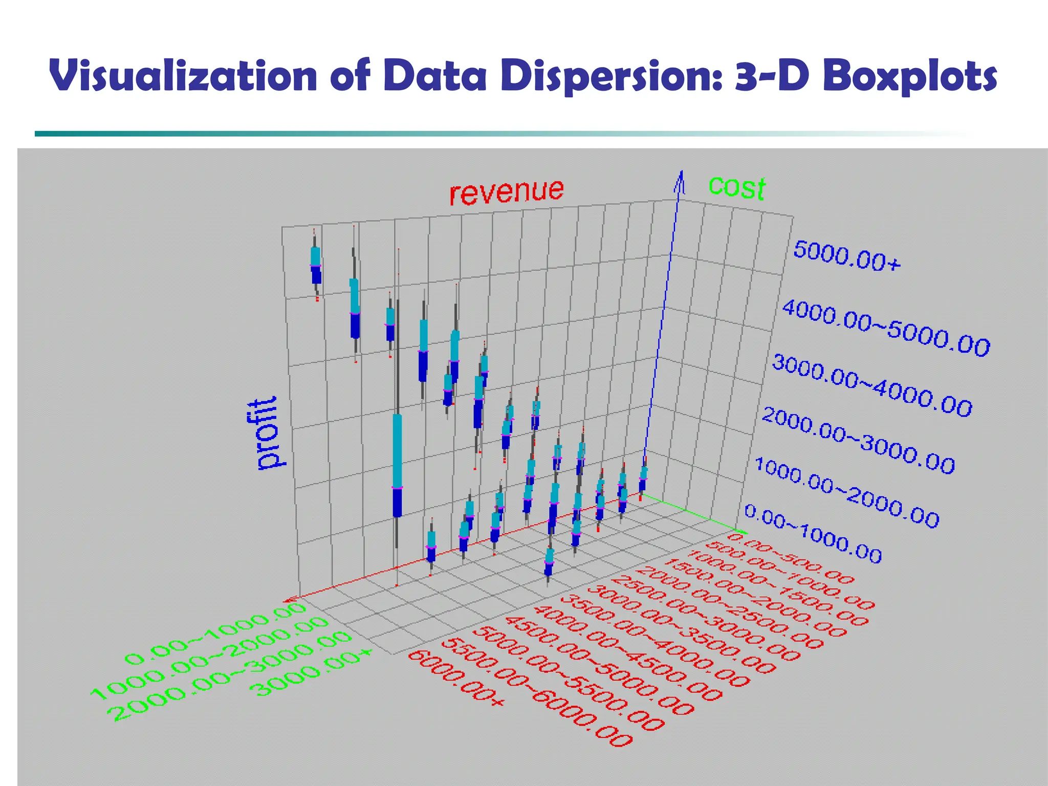
March 5, 2025Data Mining: Concepts and Techniques 16 Visualization of Data Dispersion: 3-D Boxplots
17.
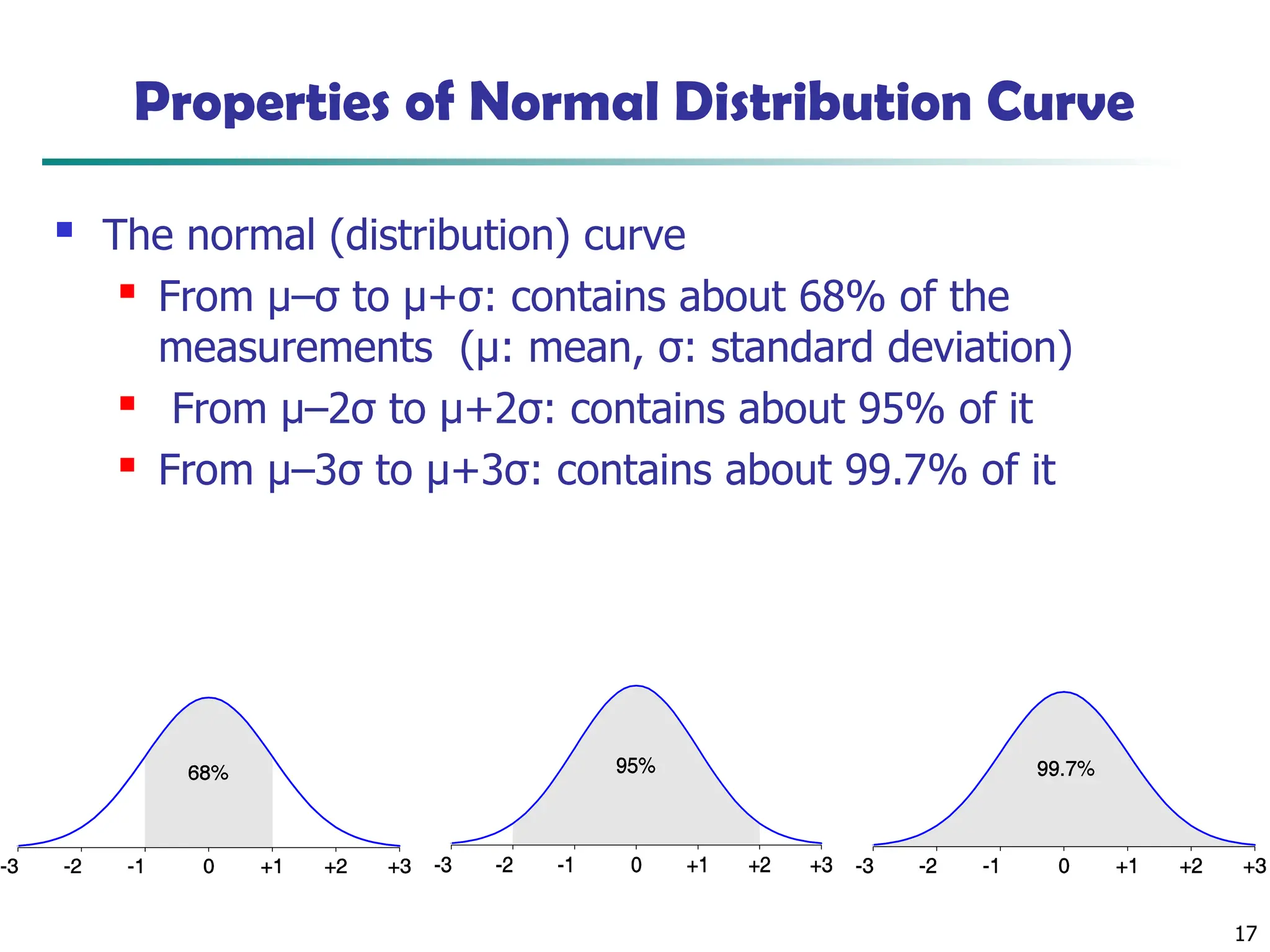
17 Properties of NormalDistribution Curve The normal (distribution) curve From μ–σ to μ+σ: contains about 68% of the measurements (μ: mean, σ: standard deviation) From μ–2σ to μ+2σ: contains about 95% of it From μ–3σ to μ+3σ: contains about 99.7% of it
18.
18 Graphic Displays ofBasic Statistical Descriptions Boxplot: graphic display of five-number summary Histogram: x-axis are values, y-axis repres. frequencies Quantile plot: each value xi is paired with fi indicating that approximately 100 fi % of data are xi Quantile-quantile (q-q) plot: graphs the quantiles of one univariant distribution against the corresponding quantiles of another Scatter plot: each pair of values is a pair of coordinates and plotted as points in the plane
19.
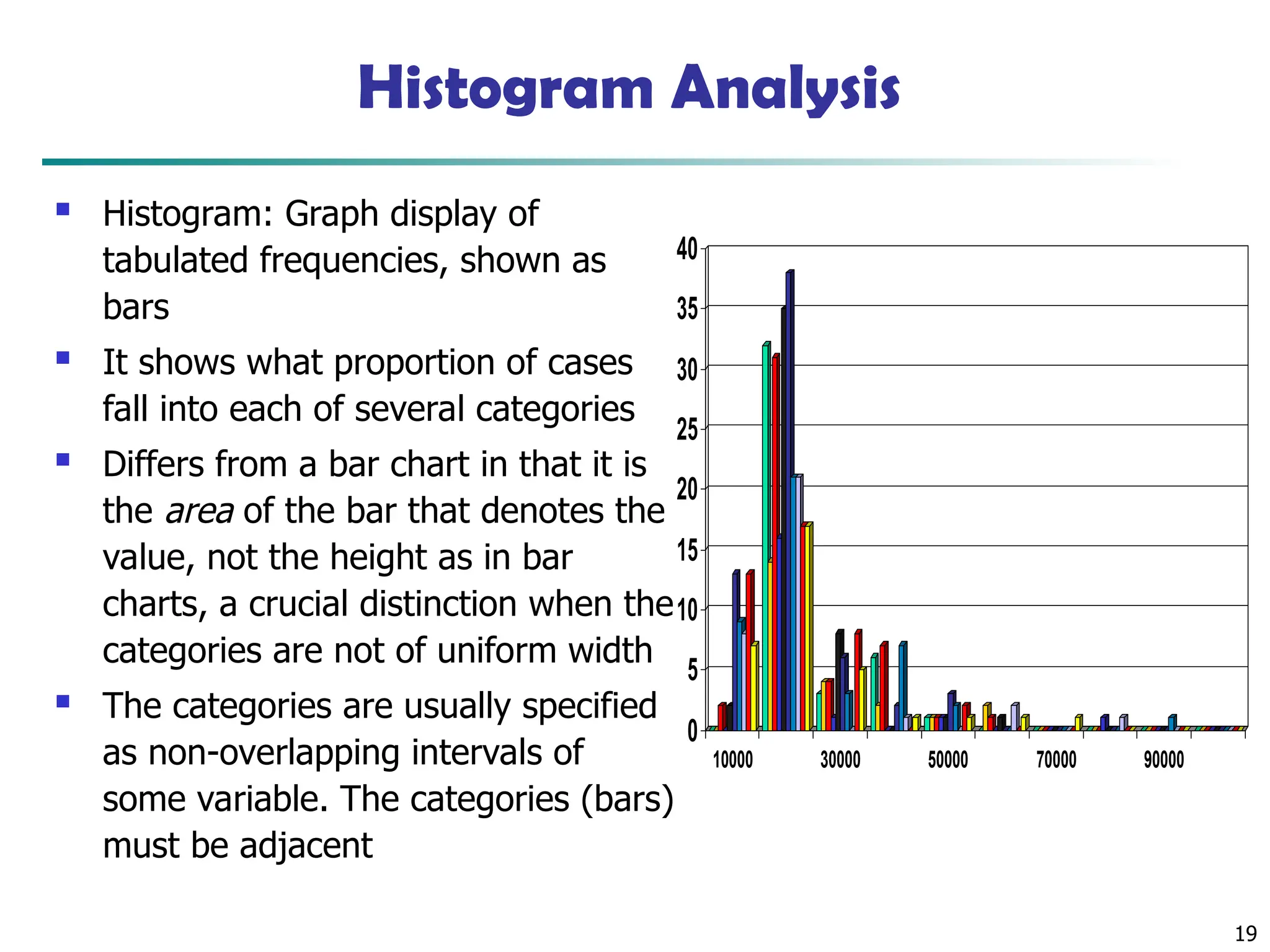
19 Histogram Analysis Histogram:Graph display of tabulated frequencies, shown as bars It shows what proportion of cases fall into each of several categories Differs from a bar chart in that it is the area of the bar that denotes the value, not the height as in bar charts, a crucial distinction when the categories are not of uniform width The categories are usually specified as non-overlapping intervals of some variable. The categories (bars) must be adjacent 0 5 10 15 20 25 30 35 40 10000 30000 50000 70000 90000
20.
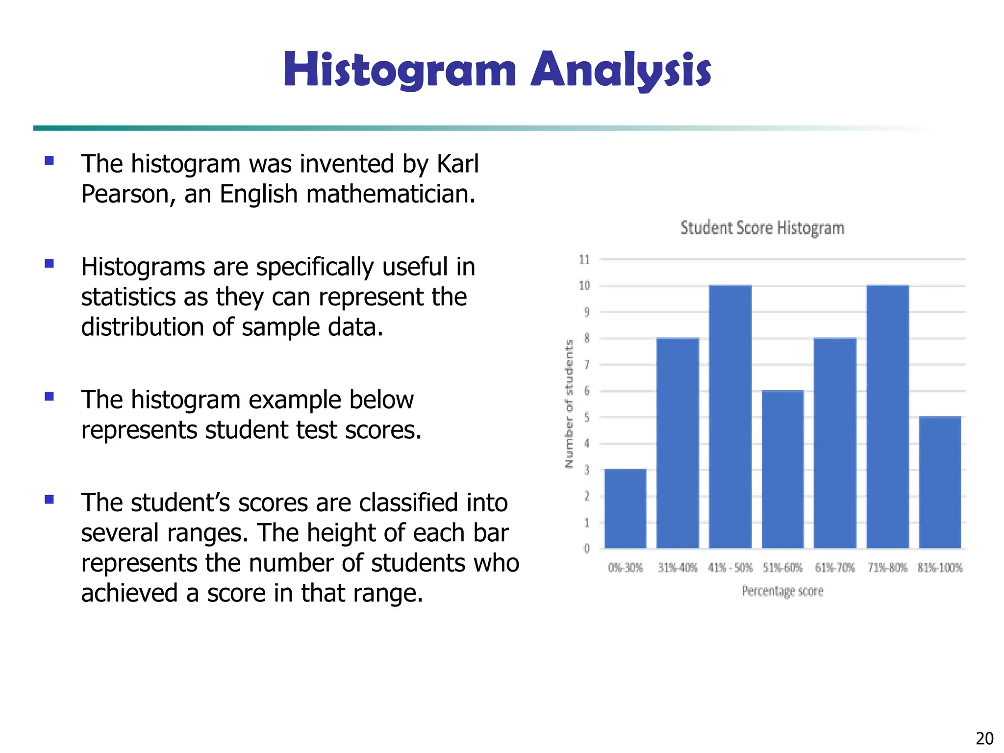
20 Histogram Analysis Thehistogram was invented by Karl Pearson, an English mathematician. Histograms are specifically useful in statistics as they can represent the distribution of sample data. The histogram example below represents student test scores. The student’s scores are classified into several ranges. The height of each bar represents the number of students who achieved a score in that range.
21.
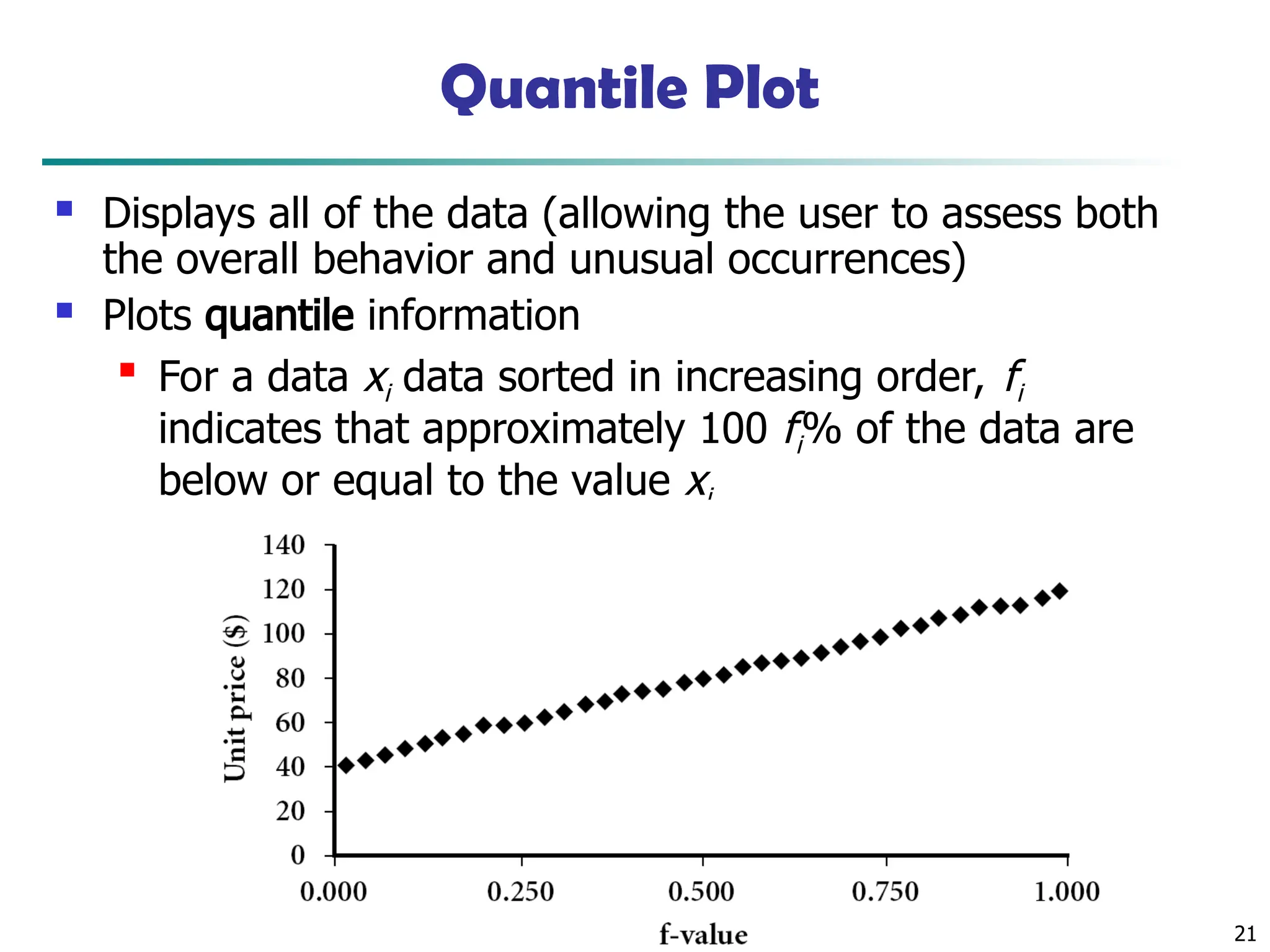
Data Mining: Conceptsand Techniques 21 Quantile Plot Displays all of the data (allowing the user to assess both the overall behavior and unusual occurrences) Plots quantile information For a data xi data sorted in increasing order, fi indicates that approximately 100 fi% of the data are below or equal to the value xi
22.
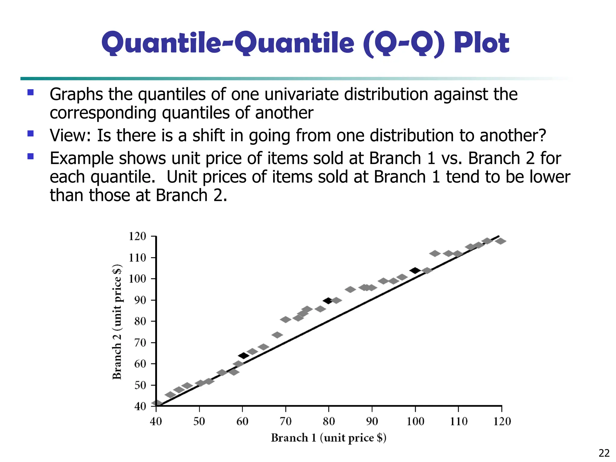
22 Quantile-Quantile (Q-Q) Plot Graphs the quantiles of one univariate distribution against the corresponding quantiles of another View: Is there is a shift in going from one distribution to another? Example shows unit price of items sold at Branch 1 vs. Branch 2 for each quantile. Unit prices of items sold at Branch 1 tend to be lower than those at Branch 2.
23.
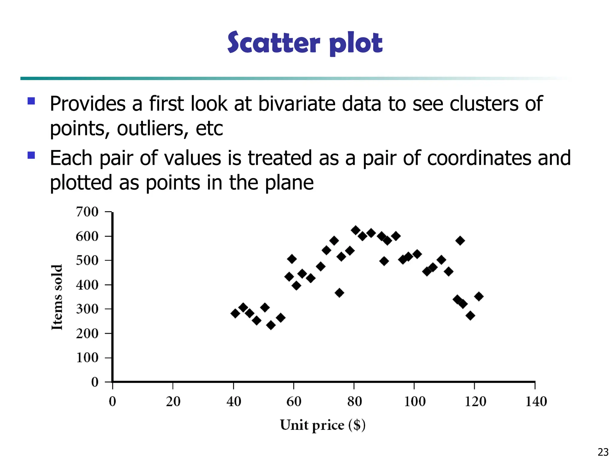
23 Scatter plot Providesa first look at bivariate data to see clusters of points, outliers, etc Each pair of values is treated as a pair of coordinates and plotted as points in the plane
24.
24 Chapter 2: Gettingto Know Your Data Data Objects and Attribute Types Basic Statistical Descriptions of Data Data Visualization Measuring Data Similarity and Dissimilarity Summary
25.
25 Chapter 2: Gettingto Know Your Data Data Objects and Attribute Types Basic Statistical Descriptions of Data Data Visualization Measuring Data Similarity and Dissimilarity Summary
26.
26 Similarity and Dissimilarity Similarity Numerical measure of how alike two data objects are Value is higher when objects are more alike Often falls in the range [0,1] Dissimilarity (e.g., distance) Numerical measure of how different two data objects are Lower when objects are more alike Minimum dissimilarity is often 0 Upper limit varies Proximity refers to a similarity or dissimilarity
27.
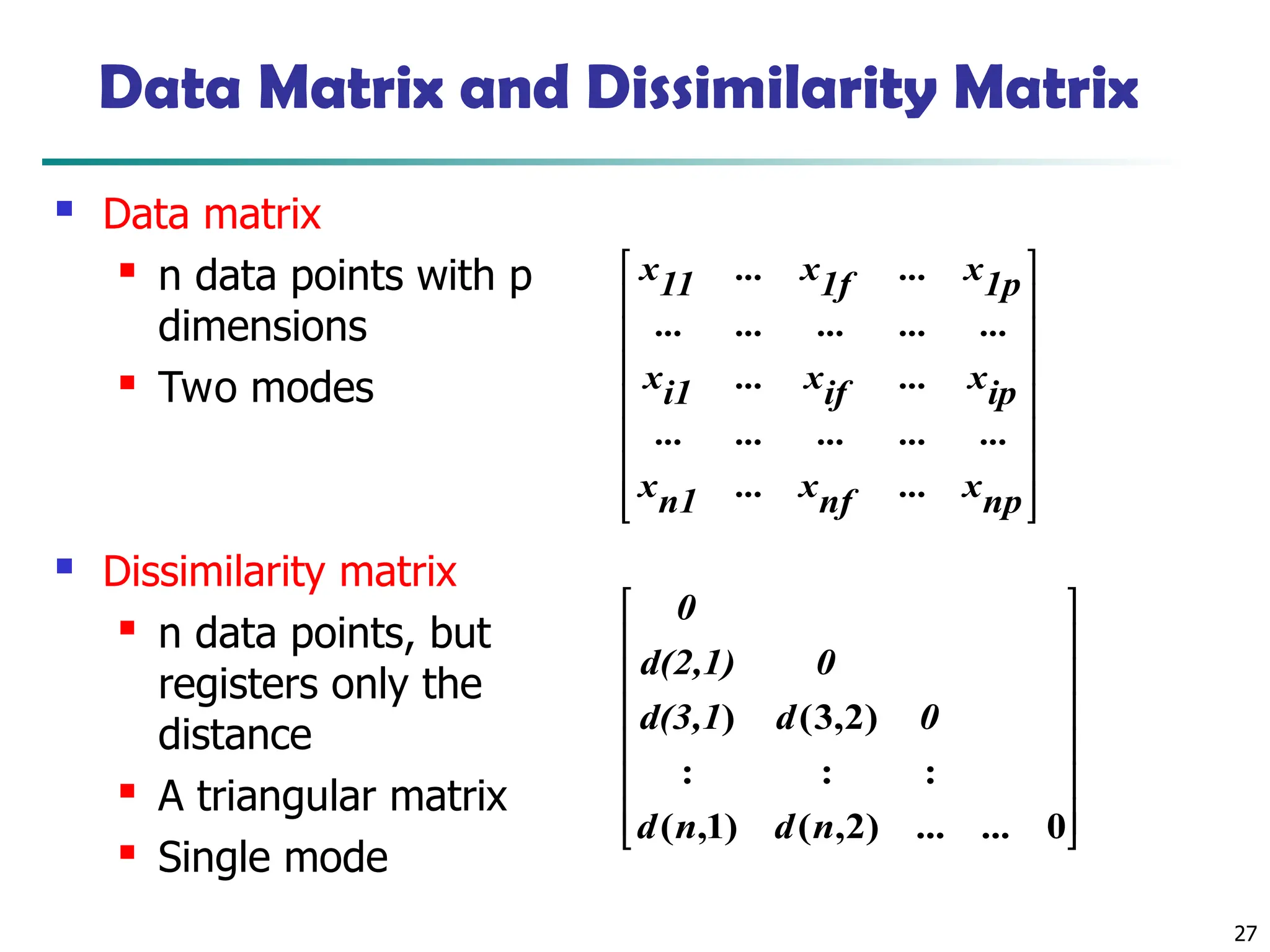
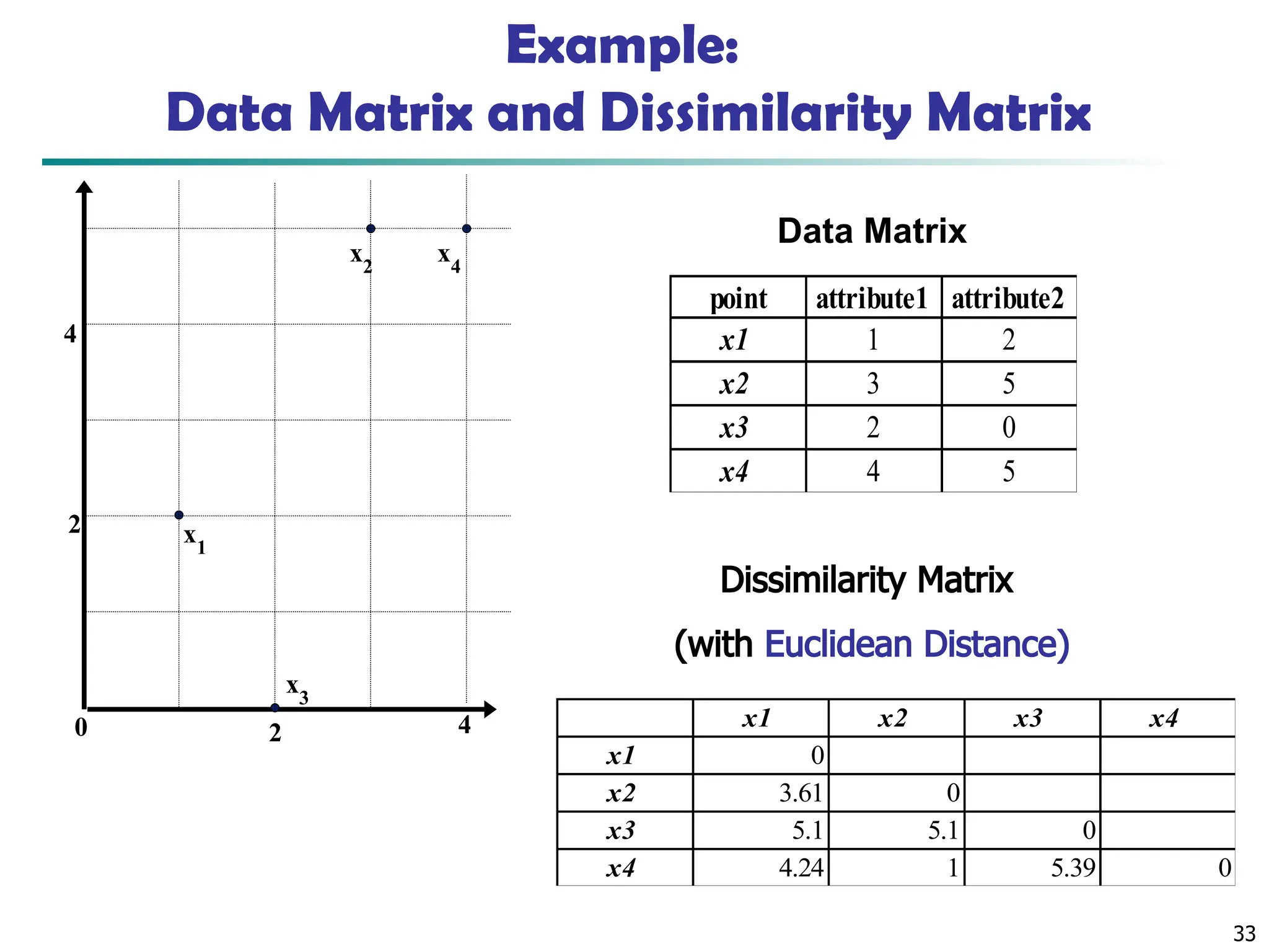
27 Data Matrix andDissimilarity Matrix Data matrix n data points with p dimensions Two modes Dissimilarity matrix n data points, but registers only the distance A triangular matrix Single mode np x ... nf x ... n1 x ... ... ... ... ... ip x ... if x ... i1 x ... ... ... ... ... 1p x ... 1f x ... 11 x 0 ... ) 2 , ( ) 1 , ( : : : ) 2 , 3 ( ) ... n d n d 0 d d(3,1 0 d(2,1) 0
28.
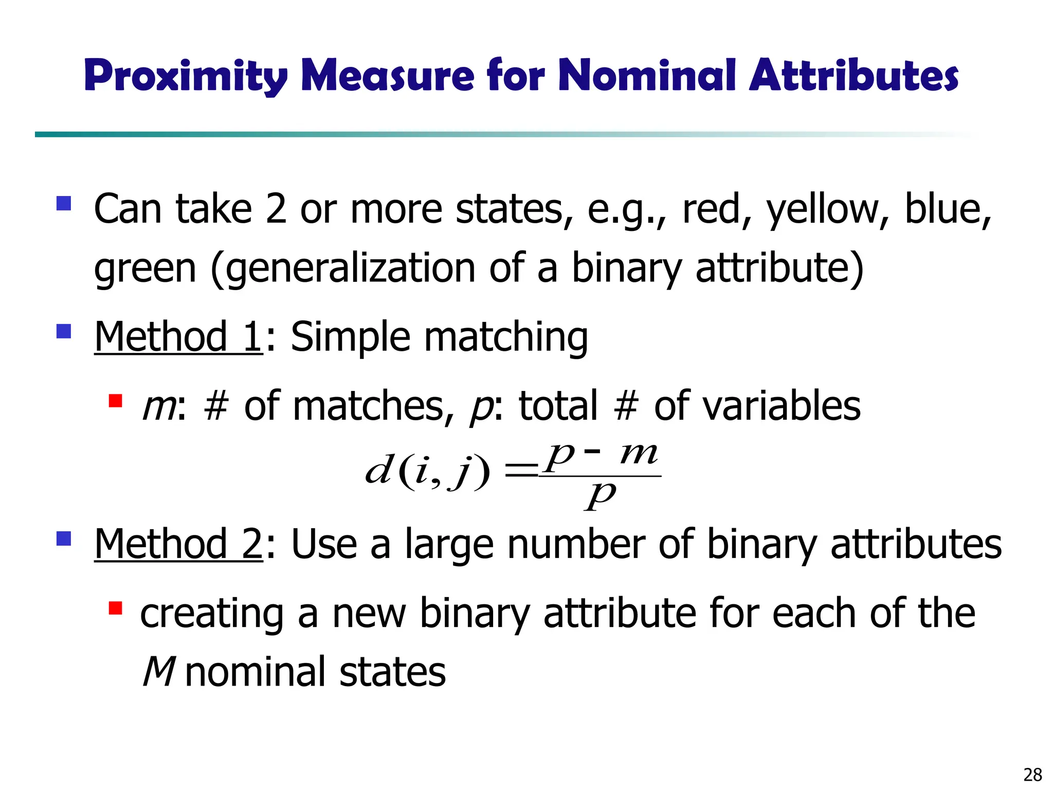
28 Proximity Measure forNominal Attributes Can take 2 or more states, e.g., red, yellow, blue, green (generalization of a binary attribute) Method 1: Simple matching m: # of matches, p: total # of variables Method 2: Use a large number of binary attributes creating a new binary attribute for each of the M nominal states p m p j i d ) , (
29.
29 Distance measure measuresinclude the Euclidean, Manhattan, and Minkowski distances. In some cases, the data are normalized before applying distance calculations Normalizing the data attempts to give all attributes an equal weight.
30.
30 Standardizing Numeric Data measures include the Euclidean, Manhattan, and Minkowski distances. In some cases, the data are normalized before applying distance calculations Normalizing the data attempts to give all attributes an equal weight. most popular distance measure is Euclidean distance
31.
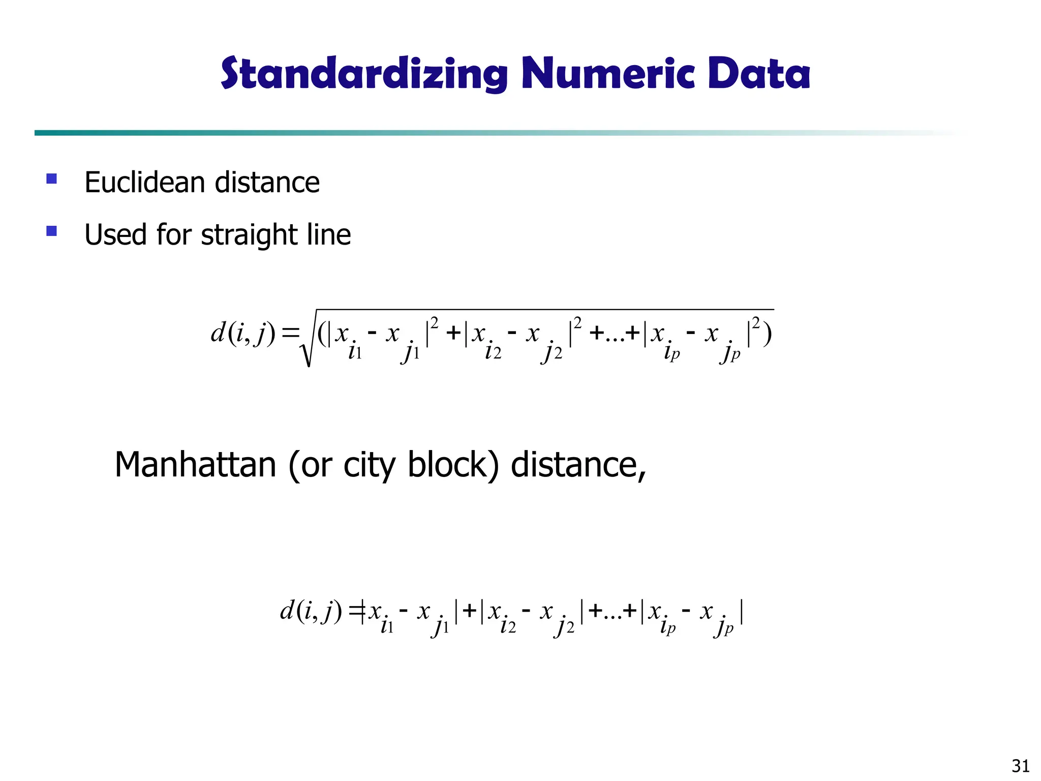
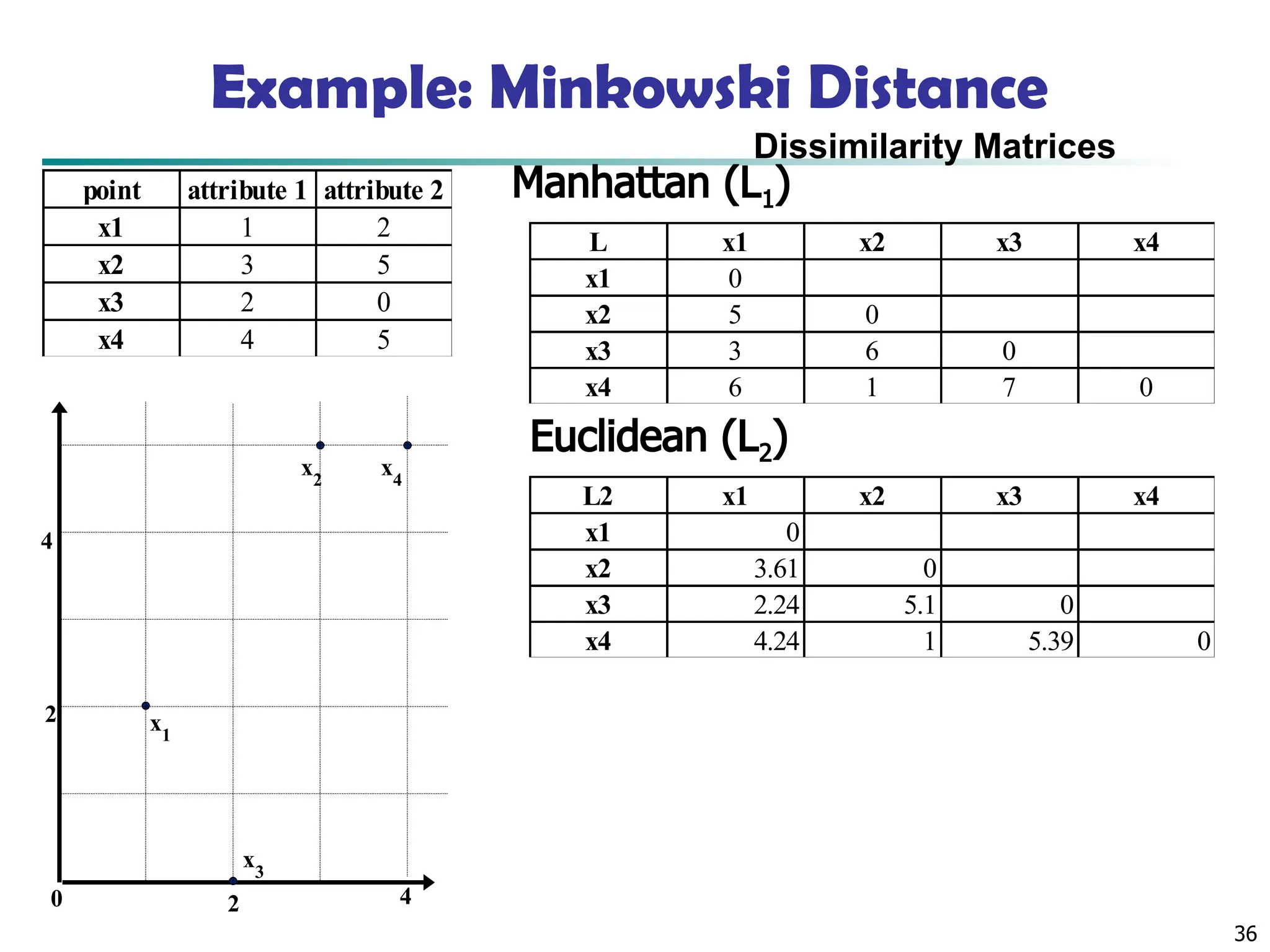
31 Standardizing Numeric Data Euclidean distance Used for straight line | | ... | | | | ) , ( 2 2 1 1 p p j x i x j x i x j x i x j i d ) | | ... | | | (| ) , ( 2 2 2 2 2 1 1 p p j x i x j x i x j x i x j i d Manhattan (or city block) distance,
32.
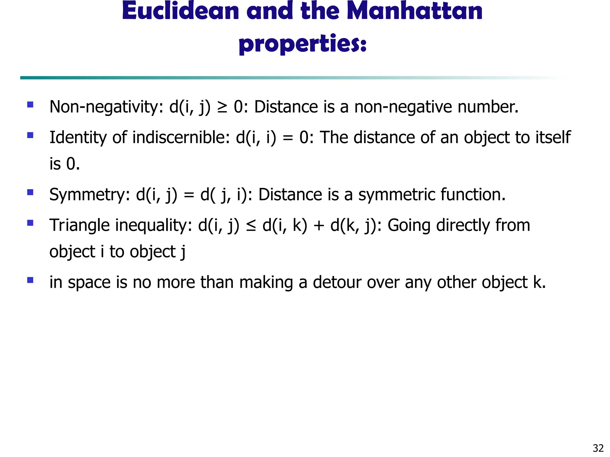
32 Euclidean and theManhattan properties: Non-negativity: d(i, j) ≥ 0: Distance is a non-negative number. Identity of indiscernible: d(i, i) = 0: The distance of an object to itself is 0. Symmetry: d(i, j) = d( j, i): Distance is a symmetric function. Triangle inequality: d(i, j) ≤ d(i, k) + d(k, j): Going directly from object i to object j in space is no more than making a detour over any other object k.
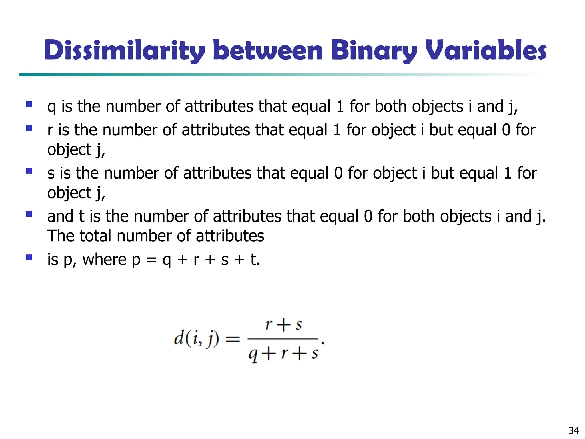
34 Dissimilarity between BinaryVariables q is the number of attributes that equal 1 for both objects i and j, r is the number of attributes that equal 1 for object i but equal 0 for object j, s is the number of attributes that equal 0 for object i but equal 1 for object j, and t is the number of attributes that equal 0 for both objects i and j. The total number of attributes is p, where p = q + r + s + t.
35.
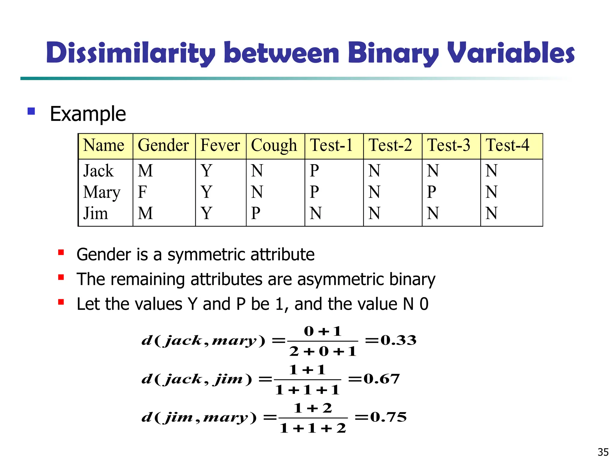
35 Dissimilarity between BinaryVariables Example Gender is a symmetric attribute The remaining attributes are asymmetric binary Let the values Y and P be 1, and the value N 0 Name Gender Fever Cough Test-1 Test-2 Test-3 Test-4 Jack M Y N P N N N Mary F Y N P N P N Jim M Y P N N N N 75 . 0 2 1 1 2 1 ) , ( 67 . 0 1 1 1 1 1 ) , ( 33 . 0 1 0 2 1 0 ) , ( mary jim d jim jack d mary jack d
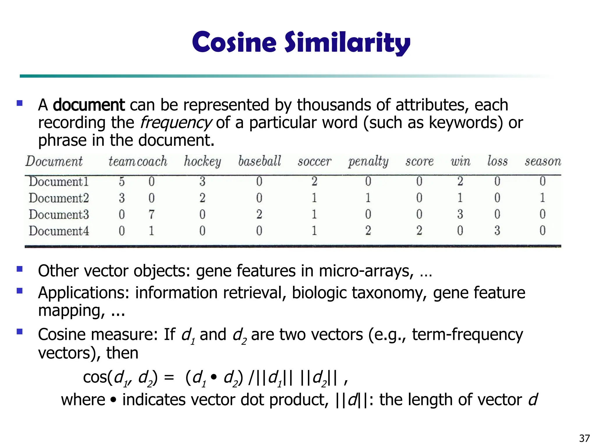
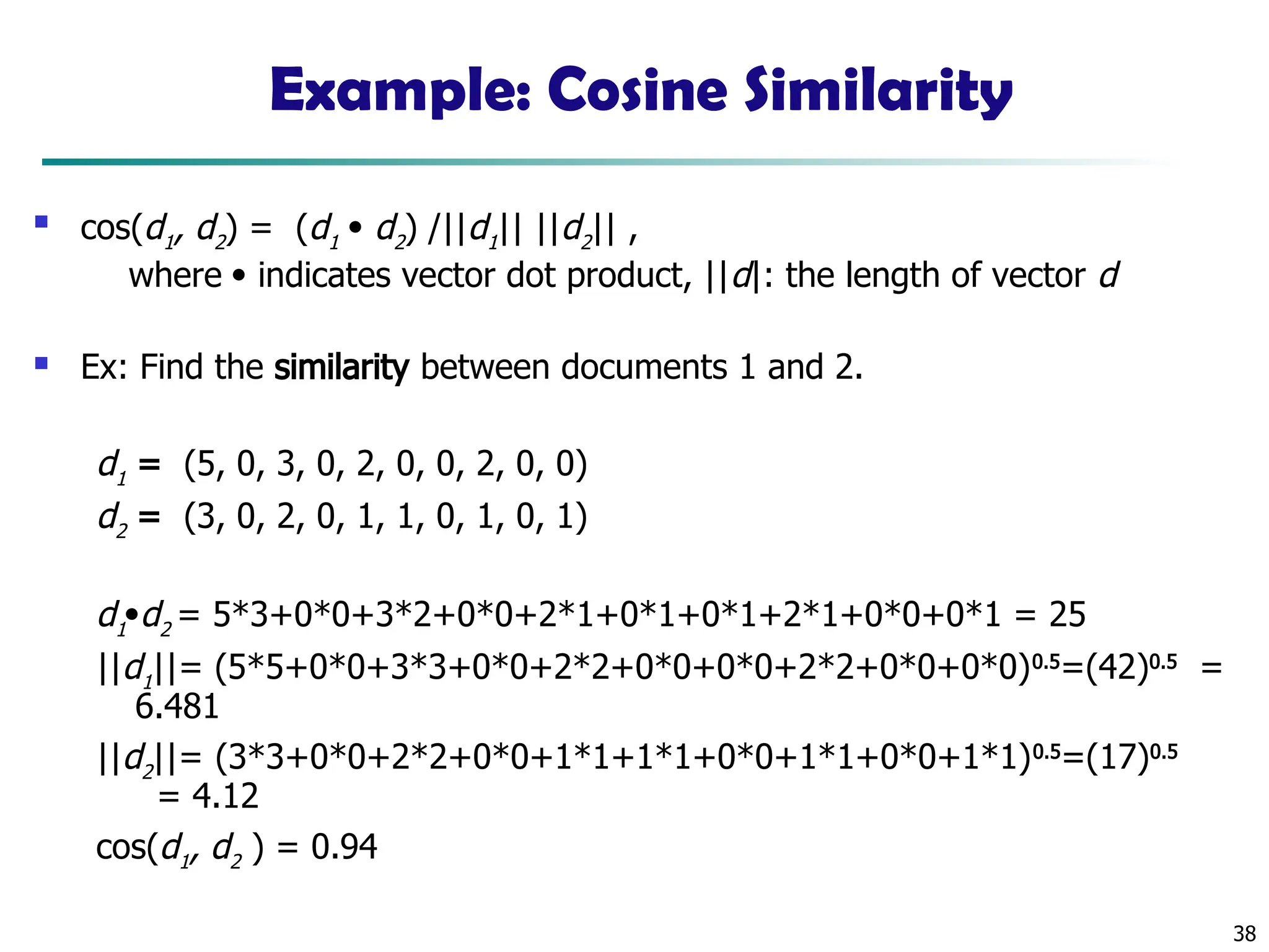
37 Cosine Similarity Adocument can be represented by thousands of attributes, each recording the frequency of a particular word (such as keywords) or phrase in the document. Other vector objects: gene features in micro-arrays, … Applications: information retrieval, biologic taxonomy, gene feature mapping, ... Cosine measure: If d1 and d2 are two vectors (e.g., term-frequency vectors), then cos(d1, d2) = (d1 d2) /||d1|| ||d2|| , where indicates vector dot product, ||d||: the length of vector d
39 Chapter 2: Gettingto Know Your Data Data Objects and Attribute Types Basic Statistical Descriptions of Data Data Visualization Measuring Data Similarity and Dissimilarity Summary
40.
Summary Data attributetypes: nominal, binary, ordinal, interval-scaled, ratio- scaled Many types of data sets, e.g., numerical, text, graph, Web, image. Gain insight into the data by: Basic statistical data description: central tendency, dispersion, graphical displays Data visualization: map data onto graphical primitives Measure data similarity Above steps are the beginning of data preprocessing. Many methods have been developed but still an active area of research. 40
41.
References W. Cleveland,Visualizing Data, Hobart Press, 1993 T. Dasu and T. Johnson. Exploratory Data Mining and Data Cleaning. John Wiley, 2003 U. Fayyad, G. Grinstein, and A. Wierse. Information Visualization in Data Mining and Knowledge Discovery, Morgan Kaufmann, 2001 L. Kaufman and P. J. Rousseeuw. Finding Groups in Data: an Introduction to Cluster Analysis. John Wiley & Sons, 1990. H. V. Jagadish, et al., Special Issue on Data Reduction Techniques. Bulletin of the Tech. Committee on Data Eng., 20(4), Dec. 1997 D. A. Keim. Information visualization and visual data mining, IEEE trans. on Visualization and Computer Graphics, 8(1), 2002 D. Pyle. Data Preparation for Data Mining. Morgan Kaufmann, 1999 S. Santini and R. Jain,” Similarity measures”, IEEE Trans. on Pattern Analysis and Machine Intelligence, 21(9), 1999 E. R. Tufte. The Visual Display of Quantitative Information, 2nd ed., Graphics Press, 2001 C. Yu , et al., Visual data mining of multimedia data for social and behavioral studies, Information Visualization, 8(1), 2009 41
Editor's Notes
#22 Note: We need to label the dark plotted points as Q1, Median, Q3 – that would help in understanding this graph. Tell audience: There is a shift in distribution of branch 1 WRT branch 2 in that the unit prices of items sold at branch 1 tend to be lower than those at branch 2.

![26 Similarity and Dissimilarity Similarity Numerical measure of how alike two data objects are Value is higher when objects are more alike Often falls in the range [0,1] Dissimilarity (e.g., distance) Numerical measure of how different two data objects are Lower when objects are more alike Minimum dissimilarity is often 0 Upper limit varies Proximity refers to a similarity or dissimilarity](https://image.slidesharecdn.com/02data1-250305121518-bc12b709/75/02Data-1-ppt-Computer-Science-Computer-Science-26-2048.jpg)