IMPROVED SWARM INTELLIGENCE APPROACH TO MULTI OBJECTIVE ED PROBLEMS

IMPROVED SWARM INTELLIGENCE APPROACH TO MULTI OBJECTIVE ED PROBLEMS

• 1.
  C.Jeevakarunya, Mrs.S.T.Suganthi /International Journal of Engineering Research and Applications (IJERA) ISSN: 2248-9622 www.ijera.com Vol. 2, Issue 2,Mar-Apr 2012, pp.1203-1211 1203 | P a g e IMPROVED SWARM INTELLIGENCE APPROACH TO MULTI OBJECTIVE ED PROBLEMS C.Jeevakarunya*, Mrs.S.T.Suganthi** *(M.E-Power system Engineering, Department of EEE, SNS college of Technology, Anna University, Coimbatore-2) ** (Assistant professor, Department of EEE, SNS college of Technology, Anna University, Coimbatore-2) ABSTRACT Electrical power industry restructuring has created highly vibrant and competitive market that altered many aspects of the power industry. In this changed scenario, scarcity of energy resources, increasing power generation cost, environment concern, ever growing demand for electrical energy necessitate optimal economic dispatch. Practical economic dispatch (ED) problems have nonlinear, non-convex type objective function with intense equality and inequality constraints. The conventional optimization methods are not able to solve such problems as due to local optimum solution convergence. Metaheuristic optimization techniques especially Improved Particle Swarm Optimization (IPSO) has gained an incredible recognition as the solution algorithm for such type of ED problems in last decade. The application of IPSO in ED problem, which is considered as one of the most complex optimization problem has been summarized in present paper. This paper illustrates successful implementation of the Improved Particle Swarm Optimization (IPSO) to Economic Load Dispatch Problem (ELD). Power output of each generating unit and optimum fuel cost obtained using IPSO algorithm has been compared with conventional techniques. The results obtained shows that IPSO algorithm converges to optimal fuel cost with reduced computational time when compared to PSO and GA for the three, six and IEEE 30 bus system. Keywords: Economic Load dispatch, Evolutionary Algorithms, GA, PSO 1. INTRODUCTION ECONOMIC dispatch (ED) problem is one of the fundamental issues in power system operation. In essence, it is an optimization problem and its objective is to reduce the total generation cost of units, while satisfying constraints. Previous efforts on solving ED problems have employed various mathematical programming methods and optimization techniques. These conventional methods include the lambda-iteration method, the base point and participation factors method, and the gradient method. [1], [2], [18], [19].In these numerical methods for solution of ED problems, an essential assumption is that the incremental cost curves of the units are monotonically increasing piecewise-linear functions. Unfortunately, this assumption may render these methods infeasible because of its nonlinear characteristics in practical systems. These nonlinear characteristics of a generator include discontinuous prohibited zones, ramp rate limits, and cost functions which are not smooth or convex. Furthermore, for a large-scale mixed-generating system, the conventional method has oscillatory problem resulting in a longer solution time. A dynamic programming (DP) method for solving the ED problem with valve-point modeling had been presented by [1], [2]. However, the DP method may cause the dimensions of the ED problem to become extremely large, thus requiring enormous computational efforts. In order to make numerical methods more convenient for solving ED problems, artificial intelligent techniques, such as the Hopfield neural networks, have been successfully employed to solve ED problems for units with piecewise quadratic fuel cost functions and prohibited zones constraint [3], [4]. However, an unsuitable sigmoidal function adopted in the Hopfield model may suffer from excessive numerical iterations, resulting in huge calculations. In the past decade, a global optimization technique known as genetic algorithms (GA) or simulated annealing (SA), which is a form of probabilistic heuristic algorithm, has been successfully used to solve power optimization problems such as feeder reconfiguration and capacitor placement in a distribution system [1],[5]–[7]. The GA method is usually faster than the SA method because the GA has parallel search techniques, which emulate natural genetic operations. Due to its high potential for global optimization, GA has received great attention in solving ED problems. In some GA applications, many constraints including network losses, ramp rate limits, and valve-point zone were considered for the practicability of the proposed method. Among these, Walters and Sheble presented a GA model that employed units‘ output as the encoded parameter of chromosome to solve an ED problem for valve-point discontinuities [5].Chen and Chang presented a GA method that used the system incremented cost as encoded parameter for solving ED problems that can take into account network losses, ramp rate limits, and valve-point zone [8]. Fung et al. presented an integrated parallel GA incorporating simulated annealing (SA) and tabu search (TS) techniques that employed the generator‘s output as the encoded parameter [9]. For an efficient GA method, Yalcinoz have used the real-coded representation scheme, arithmetic crossover, mutation, and elitism in the GA to solve more efficiently the ED problem, and it can obtain a high-quality solution with less computation time [10].
• 2.
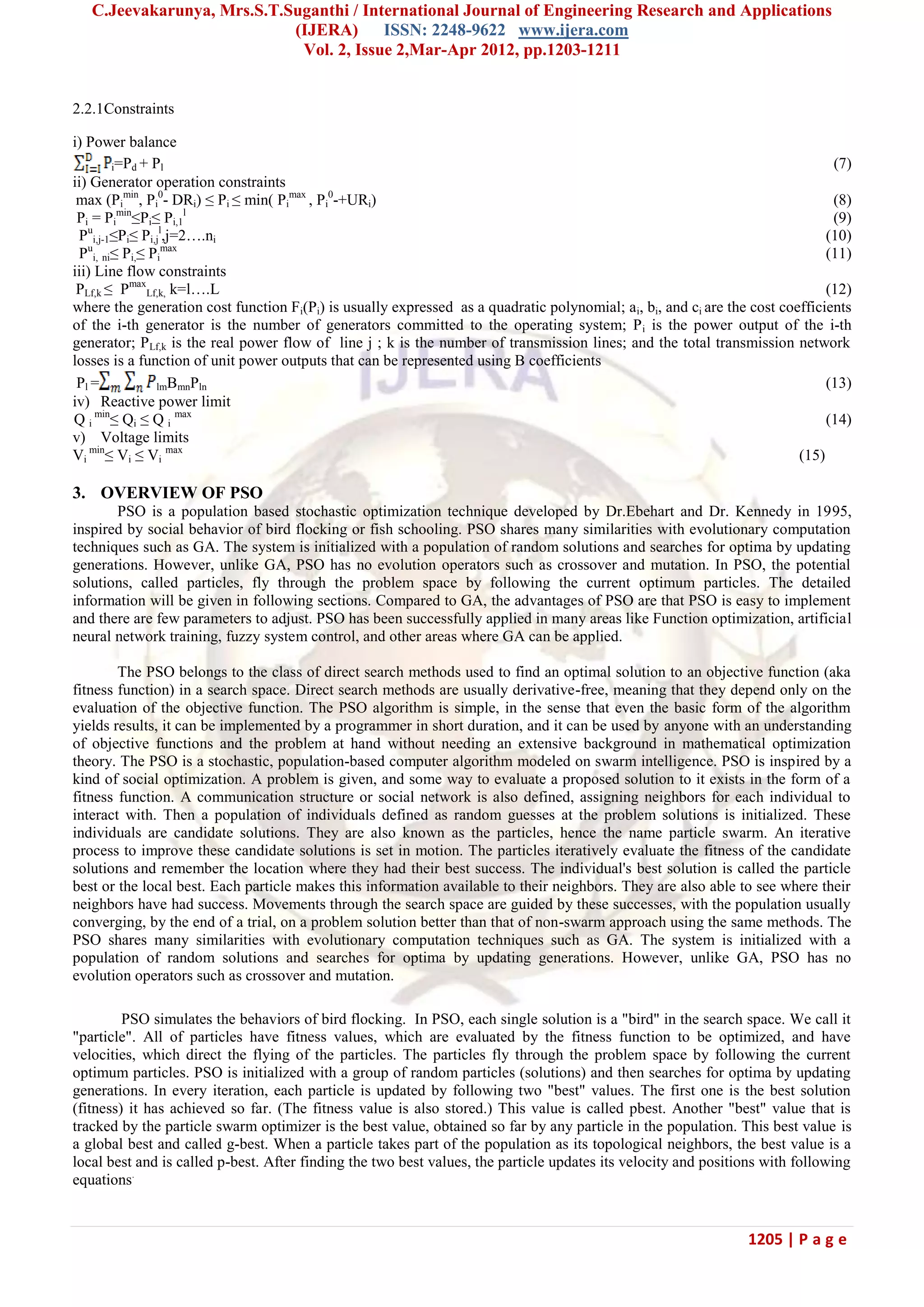
  C.Jeevakarunya, Mrs.S.T.Suganthi /International Journal of Engineering Research and Applications (IJERA) ISSN: 2248-9622 www.ijera.com Vol. 2, Issue 2,Mar-Apr 2012, pp.1203-1211 1204 | P a g e Though the GA methods have been employed successfully to solve complex optimization problems, recent research has identified some deficiencies in GA performance. This degradation in efficiency is apparent in applications with highly epistatic objective functions (i.e., where the parameters being optimized are highly correlated) [the crossover and mutation operations cannot ensure better fitness of offspring because chromosomes in the population have similar structures and their average fitness is high toward the end of the evolutionary process] [11],[16]. Moreover, the premature convergence of GA degrades its performance and reduces its search capability that leads to a higher probability toward obtaining a local optimum [11].Particle swarm optimization (PSO), first introduced by Kennedy and Eberhart, is one of the modern heuristic algorithms. It was developed through simulation of a simplified social system, and has been found to be robust in solving continuous nonlinear optimization problems [13]–[17]. The PSO technique can generate high-quality solutions within shorter calculation time and stable convergence characteristic than other stochastic methods [14]–[17]. Although the PSO seems to be sensitive to the tuning of some weights or parameters, many researches are still in progress for proving its potential in solving complex power system problems [16]. Researchers including Yoshida et al. have presented a PSO for reactive power and voltage control (VC) considering voltage security assessment. The feasibility of their method is compared with the reactive tabu system (RTS) and enumeration method on practical power system, and has shown promising results [18].Naka et al. have presented the use of a hybrid PSO method for solving efficiently the practical distribution state estimation problem [19]. In this paper, a PSO method for solving the ED problem in power system is proposed. The proposed method considers the nonlinear characteristics of a generator such as ramp rate limits and prohibited operating zone for actual power system operation. The feasibility of the proposed method was demonstrated for three different systems [8], [20], respectively. 2. PROBLEM DESCRIPTION The ED is one sub problem of the unit commitment (UC) problem. It is a nonlinear programming optimization one. Practically, while the scheduled combination units at each specific period of operation are listed, the ED planning must perform the optimal generation dispatch among the operating units to satisfy the system load demand, spinning reserve capacity, and practical operation constraints of generators that include the ramp rate limit and the prohibited operating zone [12]. 2.1 Practical Operation Constraints of Generator For convenience in solving the ED problem, the unit generation output is usually assumed to be adjusted smoothly and instantaneously. Practically, the operating range of all online units is restricted by their ramp rate limits for forcing the units operation continually between two adjacent specific operation periods [1], [2]. In addition, the prohibited operating zones in the input-output curve of generator are due to steam valve operation or vibration in a shaft bearing. Because it is difficult to determine the prohibited zone by actual performance testing or operating records, the best economy is achieved by avoiding operation in areas that are in actual operation. Hence, the two constraints of generator operation must be taken into account to achieve true economic operation. 2.1.1) Ramp Rate Limit: According to [3], [5], and [8], the inequality constraints due to ramp rate limits for unit generation changes are given a) As generation increases Pi-Pi 0 ≤URi (1) b) As generation decreases Pi-Pi 0 ≤DRi (2) Where Pi is the current output power and Pi 0 is the previous output power. URi is the up ramp limit of the i-th generator (MW/time-period); and DRi is the down ramp limit of the i-th generator (MW/time period). 2.1.2) Prohibited Operating Zone: References [2], [3], and [8] have shown the input-output performance curve for a typical thermal unit with many valve points. These valve points generate many prohibited zones. In practical operation, adjusting the generation output Pi of a unit must avoid unit operation in the prohibited zones. The feasible operating zones of unit can be described as follows: Pi min ≤Pi≤ Pi,1 l (3) Pi,j-1 u ≤Pi≤ Pi,j l ,j=2….ni (4) Pi, ni u ≤ Pi,≤ Pi max (5) 2.2 OBJECTIVE FUNCTION The objective of ED is to simultaneously minimize the generation cost rate and to meet the load demand of a power system over some appropriate period while satisfying various constraints. To combine the above two constraints into a ED problem, the constrained optimization problem at specific operating interval can be modified as Minimize F t = = ai (Pi 2 ) +bi(Pi)+ci (6)
• 3.
  C.Jeevakarunya, Mrs.S.T.Suganthi /International Journal of Engineering Research and Applications (IJERA) ISSN: 2248-9622 www.ijera.com Vol. 2, Issue 2,Mar-Apr 2012, pp.1203-1211 1205 | P a g e 2.2.1Constraints i) Power balance i=Pd + Pl (7) ii) Generator operation constraints max (Pi min , Pi 0 - DRi) ≤ Pi ≤ min( Pi max , Pi 0 -+URi) (8) Pi = Pi min ≤Pi≤ Pi,1 l (9) Pu i,j-1≤Pi≤ Pi,j l ,j=2….ni (10) Pu i, ni≤ Pi,≤ Pi max (11) iii) Line flow constraints PLf,k ≤ Pmax Lf,k, k=l….L (12) where the generation cost function Fi(Pi) is usually expressed as a quadratic polynomial; ai, bi, and ci are the cost coefficients of the i-th generator is the number of generators committed to the operating system; Pi is the power output of the i-th generator; PLf,k is the real power flow of line j ; k is the number of transmission lines; and the total transmission network losses is a function of unit power outputs that can be represented using B coefficients Pl = lmBmnPln (13) iv) Reactive power limit Q i min ≤ Qi ≤ Q i max (14) v) Voltage limits Vi min ≤ Vi ≤ Vi max (15) 3. OVERVIEW OF PSO PSO is a population based stochastic optimization technique developed by Dr.Ebehart and Dr. Kennedy in 1995, inspired by social behavior of bird flocking or fish schooling. PSO shares many similarities with evolutionary computation techniques such as GA. The system is initialized with a population of random solutions and searches for optima by updating generations. However, unlike GA, PSO has no evolution operators such as crossover and mutation. In PSO, the potential solutions, called particles, fly through the problem space by following the current optimum particles. The detailed information will be given in following sections. Compared to GA, the advantages of PSO are that PSO is easy to implement and there are few parameters to adjust. PSO has been successfully applied in many areas like Function optimization, artificial neural network training, fuzzy system control, and other areas where GA can be applied. The PSO belongs to the class of direct search methods used to find an optimal solution to an objective function (aka fitness function) in a search space. Direct search methods are usually derivative-free, meaning that they depend only on the evaluation of the objective function. The PSO algorithm is simple, in the sense that even the basic form of the algorithm yields results, it can be implemented by a programmer in short duration, and it can be used by anyone with an understanding of objective functions and the problem at hand without needing an extensive background in mathematical optimization theory. The PSO is a stochastic, population-based computer algorithm modeled on swarm intelligence. PSO is inspired by a kind of social optimization. A problem is given, and some way to evaluate a proposed solution to it exists in the form of a fitness function. A communication structure or social network is also defined, assigning neighbors for each individual to interact with. Then a population of individuals defined as random guesses at the problem solutions is initialized. These individuals are candidate solutions. They are also known as the particles, hence the name particle swarm. An iterative process to improve these candidate solutions is set in motion. The particles iteratively evaluate the fitness of the candidate solutions and remember the location where they had their best success. The individual's best solution is called the particle best or the local best. Each particle makes this information available to their neighbors. They are also able to see where their neighbors have had success. Movements through the search space are guided by these successes, with the population usually converging, by the end of a trial, on a problem solution better than that of non-swarm approach using the same methods. The PSO shares many similarities with evolutionary computation techniques such as GA. The system is initialized with a population of random solutions and searches for optima by updating generations. However, unlike GA, PSO has no evolution operators such as crossover and mutation. PSO simulates the behaviors of bird flocking. In PSO, each single solution is a "bird" in the search space. We call it "particle". All of particles have fitness values, which are evaluated by the fitness function to be optimized, and have velocities, which direct the flying of the particles. The particles fly through the problem space by following the current optimum particles. PSO is initialized with a group of random particles (solutions) and then searches for optima by updating generations. In every iteration, each particle is updated by following two "best" values. The first one is the best solution (fitness) it has achieved so far. (The fitness value is also stored.) This value is called pbest. Another "best" value that is tracked by the particle swarm optimizer is the best value, obtained so far by any particle in the population. This best value is a global best and called g-best. When a particle takes part of the population as its topological neighbors, the best value is a local best and is called p-best. After finding the two best values, the particle updates its velocity and positions with following equations.
• 4.
  C.Jeevakarunya, Mrs.S.T.Suganthi /International Journal of Engineering Research and Applications (IJERA) ISSN: 2248-9622 www.ijera.com Vol. 2, Issue 2,Mar-Apr 2012, pp.1203-1211 1206 | P a g e Vi (u+1) =W*Vi (u) +C1*rand()*(pbesti-Pi (u) )+ C2*rand()*(gbesti-Pi (u) ) (16) Pi (u+1) =Pi (u) + Vi (u+1) (17) In the above equation, The term rand ( )*(pbest i -Pi (u) ) is called particle memory influence The term rand ( )*( gbesti -Pi (u) ) is called swarm influence. Vi (u) which is the velocity of ith particle at iteration ‗u‘ must lie in the range Vmin ≤ Vi (u) ≤ Vmax The parameter Vmax determines the resolution, or fitness, with which regions are to be searched between the present position and the target position a. If Vmax is too high, particles may fly past good solutions. If Vmin is too small, particles may not explore sufficiently beyond local solutions. b. In many experiences with PSO, Vmax was often set at 10-20% of the dynamic range on each dimension. c. The constants C1and C2 pull each particle towards pbest and gbest positions. d. Low values allow particles to roam far from the target regions before being tugged back. On the other hand, high values result in abrupt movement towards, or past, target regions. e. The acceleration constants C1 and C2 are often set to be 2.0 according to past experiences f. Suitable selection of inertia weight ‘ω‘ provides a balance between global and local explorations, thus requiring less iteration on average to find a sufficiently optimal solution. In general, the inertia weight w is set according to the following equation, (18) where w -is the inertia weighting factor Wmax - maximum value of weighting factor Wmin - minimum value of weighting factor ITERmax - maximum number of iterations ITER - current number of iteration The Equation (5.1) is used to calculate the particle's new velocity according to its previous velocity and the distances of its current position from its own best experience (position) and the group's best experience. Then the particle flies towards a new position according to Equation (2). The performance of each particle is measured according to a predefined fitness function , this is related to the problem to be solved. The step by step procedure of PSO algorithm is given as follows a. Initialize a population of particles with random values and velocities within the d-dimensional search space. Initialize the maximum allowable velocity magnitude of any particle Vmax. Evaluate the fitness of each particle and assign the particle's position to pbest position and fitness to pbest fitness. Identify the best among the pbest as gbest. b. Change the velocity and position of the particle according to Equations (5.1) and Equations (5.2) respectively. c. For each particle, evaluate the fitness, if all decisions variables are within the search ranges. d. Compare the particle's fitness evaluation with its previous pbest. If the current value is better than the previous pbest, then set the pbest value equal to the current value and the pbest location equal to the current location in the d dimensional search space. e. Compare the best current fitness evaluation with the population gbest. If the current value is better than the population gbest, then reset the gbest to the current best position and the fitness value to current fitness value. f. Repeat steps 2-5 until a stopping criterion, such as sufficiently good gbest fitness or a maximum number of iterations i function evaluations is met. 4. PSO IMPLEMENTATION TO ELD When the losses are considered the optimization process becomes little bit complicated. Since the losses are dependent on the power generated of the each unit, in each generation the loss changes. The P-loss can be found out by using the equation (19)
• 5.
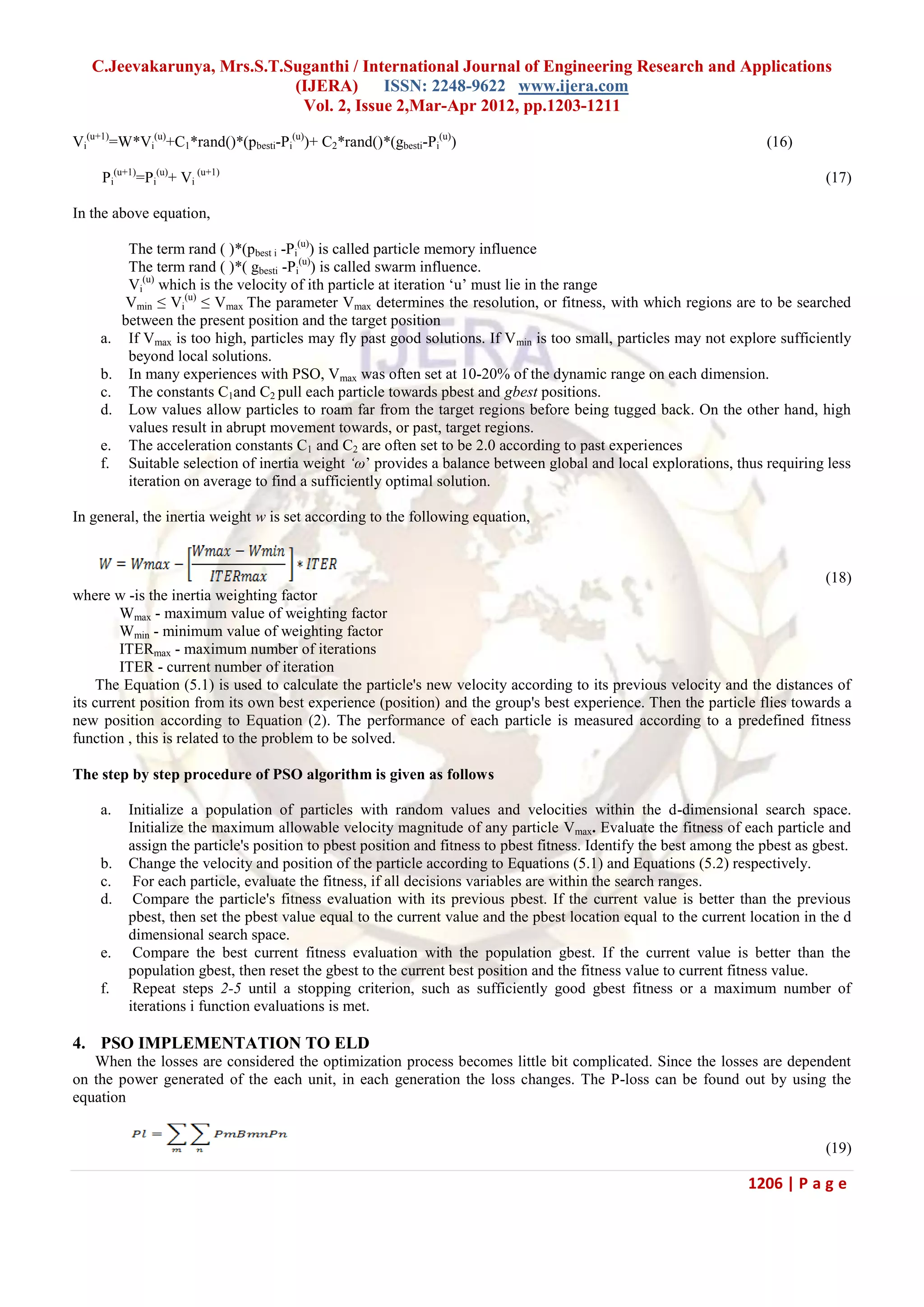
  C.Jeevakarunya, Mrs.S.T.Suganthi /International Journal of Engineering Research and Applications (IJERA) ISSN: 2248-9622 www.ijera.com Vol. 2, Issue 2,Mar-Apr 2012, pp.1203-1211 1207 | P a g e Where Bmn are the loss co-efficient. The loss co-efficient can be calculated from the load flow equations or it may be given in the problem. However in this work for simplicity the loss coefficient are given which are the approximate one. Some parts are neglected. The sequential steps to find the optimum solution are a. The power of each unit, velocity of particles, is randomly generated which must be in the maximum and minimum limit. These initial individuals must be feasible candidate solutions that satisfy the practical operation constraints. b. Each set of solution in the space should satisfy the following equation i=Pd + Pl (20) Pl calculated by using above equation .Then equality constraints are checked. If any c. Combination doesn‘t satisfy the constraints then they are set according to the power balance equation. (21) d. The cost function of each individual Pgi, is calculated in the population using the evaluation function F. Here F is F=a*(Pgi) 2 +b*Pgi +c (22) where a, b, c are constants. The present value is set as the pbest value. e. Each pbest values are compared with the other pbest values in the population. The best evaluation value among the pbest is denoted as gbest. f. The member velocity v of each individual Pg is updated according to the velocity update equation Vid (u+1) =w *Vi (u) +C1*rand ( )*(pbest id -Pgid (u) +C2*rand ( )*( gbestid -Pgid (u) ) (23) where u is the number of iteration. g. The velocity components constraint occurring in the limits from the following conditions are checked Vdmin = -0.5*Pmin (24) Vdmax = +0.5*Pmax (25) h. The position of each individual Pg is modified according to the position update equation P gid (u+1) = P gid (u) + V id (u+1) (26) i. The cost function of each new is calculated If the evaluation value of each individual is better than previous pbest; the current value is set to be pbest. If the best pbest is better than gbest, the value is set to be gbest. j. If the number of iterations reaches the maximum, then go to step 10.Otherwise, go to step 2. k. The individual that generates the latest gbest is the optimal generation power of each unit with the minimum total generation cost. 5. IMPROVED SWARM INTELLIGENCE APPROACH TO ELD Especially, most of the PSO algorithms are aimed at unconstrained problems. For the constrained problems, the approach introduced is just the traditional combination of primitive PSO and the penalty function. It was investigated that the simple penalty function strategy cannot be integrated well with PSO algorithms because it does not utilize the historical memory information, which is an essential of PSO. Besides penalty functions face the difficulty of maintaining a balance between obtaining feasibility even as finding optimality. Thus, in order to solve constrained ELD problem optimization a new constraints handling strategy is used for improvement the optimization mechanism of PSO algorithm. The proposed approach is called preservation of Feasible Solutions Method (FSM). This method for constraint handling with PSO was adapted by Hu and Eberhart in [8]. In the proposed method, fitness function and constraints are handled separately. Fitness function is used to guide search direction. Constraints are used to check the feasibility of particles. When implementing this technique into the global version of PSO, the initialization process involves forcing all particles into the feasible space before any evaluation of the objective function has begun. Upon evaluation of the objective function, only particles which remain in the feasible space are counted for the new PBest and GBest values (or lBest for the local version).Although extra loops are needed to find feasible solutions, the time complexity is not high as expected. A feasible solution has to satisfy all the constraints. Once a constraint is not satisfied, it is not necessary to test other constraints. Thus, the overall time complexity is not proportional to the number of needed loops and the computation time will be much less. The idea here is to accelerate the
• 6.
  C.Jeevakarunya, Mrs.S.T.Suganthi /International Journal of Engineering Research and Applications (IJERA) ISSN: 2248-9622 www.ijera.com Vol. 2, Issue 2,Mar-Apr 2012, pp.1203-1211 1208 | P a g e iterative process of tracking feasible solutions by forcing the search space to contain only solutions that do not violate any constraints. The process of the modified PSO algorithm for solution of the ELD problem can be summarized as follows: a. Read the original data including power system data and the PSO parameters. b. Set the generation counter t=0, Initialize randomly the particles of the population, Repeat initializing particle until it satisfies all the constraints. Note that it is very important to create a group of individuals satisfying the equality constraint (3) and inequality constraints (4). i.e.: summation of all elements of individual i. P and the created element of individual at random should be located within its boundary. Although, we can create element of individual at random satisfying the inequality constraint by mapping [0, 1] into [Pmax-Pmin], the particles are randomly generated between the maximum and the minimum operating limits of the generators. In the ED problems the number of online generating units is the ‗dimension‘ of this problem. For example, if there are N units, the i th particle is represented as follows: Pi = ( Pi1 , Pi2 , Pi3 , . . . , PiN ). c. The particle velocities are generated randomly in the range[-Vj max ,Vj max ].The maximum velocity limit in the jth dimension is computed as follows: Vj max= , max , minj jX X R  (27) Where, R is the chosen number of intervals in the jth dimension. For all the examples tested using the PSO approach, Vmax was set at 10–20% of the dynamic range of the variable on each dimension. d. Calculate the evaluation value of each particle, in the population using the evaluation function (1) as initial fitness and set initial position particles as the initial Pbest value of the particles. The initial best value among the particle swarm is set to initial Gbest. e. Let t=t+1. f. update velocities and positions for all the dimensions in each particle by Eq. (16).and (17). g. Calculate the fitness value of the new particles by power flow calculation and object function. h. Update Pbest by using preserving feasibility strategy.If the new value is better than the previous Pbest and the particle is in the feasible space, then the new value is set to Pbest and then selected the particle with the best Pbest value among all the swarm as the Gbest. i. The best value among all the Pbest values, Gbest, is identified. j. Go to step (5) until a termination criterion is met, usually a sufficiently good fitness value or a maximum number of generation is chosen for termination criterion. 5. SIMULATION RESULTS The applicability and validity of the PSO algorithm for practical applications has been tested on various test cases. The obtained best solution in fifty runs are compared with the results obtained using GA [2]. All the programs are developed using MATLAB 7.01 and the system configuration is Intel Core 2 Duo with 4 GHz speed and 4GB RAM. In this section, to demonstrate the effectiveness of the proposed method, the IPSO are applied to solve the three, six, and thirty bus systems by considering the constraints of the ED problem. The simulation results are compared with PSO and GA method reported in literature. The parameters of the IPSO such as c1 and c2 are set as 2.05, K =0.729 , Vmin =0.4, Vmax =0.9, Table I, II, III shows the data of the test system. The best results obtained from the IPSO are compared with the PSO and GA. The results show that the proposed approaches have high solution quality than others method as depicted. Table IV, V, VI shows the effectiveness in term of the solution quality among 100 trials of proposed methods. The solutions of the proposed methods higher quality than the rest methods in term of minimum cost, average cost, maximum cost, computational time and solution deviation. The cost coefficients and generation limits of three units system are taken from [2]. Transmission loss for this system is calculated using matrix. TABLE I GENERATING UNIT CAPACITY AND COEFFICIENTS: THREE GENERATING UNIT SYSTEM a i ($/MWh 2 ) b i ($/MWh) c i P min (MW) P max (MW) 0.008 7 200 10 85 0.009 6.3 180 10 80
• 7.
  C.Jeevakarunya, Mrs.S.T.Suganthi /International Journal of Engineering Research and Applications (IJERA) ISSN: 2248-9622 www.ijera.com Vol. 2, Issue 2,Mar-Apr 2012, pp.1203-1211 1209 | P a g e 0.007 6.8 140 10 70 ai,bi,ci are the fuel cost coefficients and Pmax and Pmin are the real power limits. TABLE II SIX GENERATING UNIT SYSTEM a i ($/MWh 2 ) b i ($/MWh) c i P min (MW) P max (MW) 0.0070 7 240 100 500 0.0095 10 200 50 200 0.0090 8.5 220 80 300 0.0090 11 200 50 150 0.0080 10.5 220 50 200 0.0075 12 120 50 120 TABLE III IEEE 30 BUS SYSTEM UNIT S p i MAX (MW) p i MIN (MW) a i ($/MWh 2 ) b i ($/MWh) C i 1 50 200 0.00375 2.00 0 2 20 80 0.01750 1.75 0 5 15 50 0.06250 1.00 0 8 10 35 0.00834 3.25 0 11 10 30 0.02500 3.00 0 13 12 40 0.02500 3.00 0 The results including the generation cost, and power losses are shown below. The result gives the optimum generations for minimum total cost and seems to be efficient for solving non convex ELD problems. The IPSO algorithms were tested and the results were presented for various test systems. Results showed that IPSO methods are well suited for obtaining the best solution for fuel cost functions of differentiable, non smooth, and non differentiable of the test systems.
• 8.
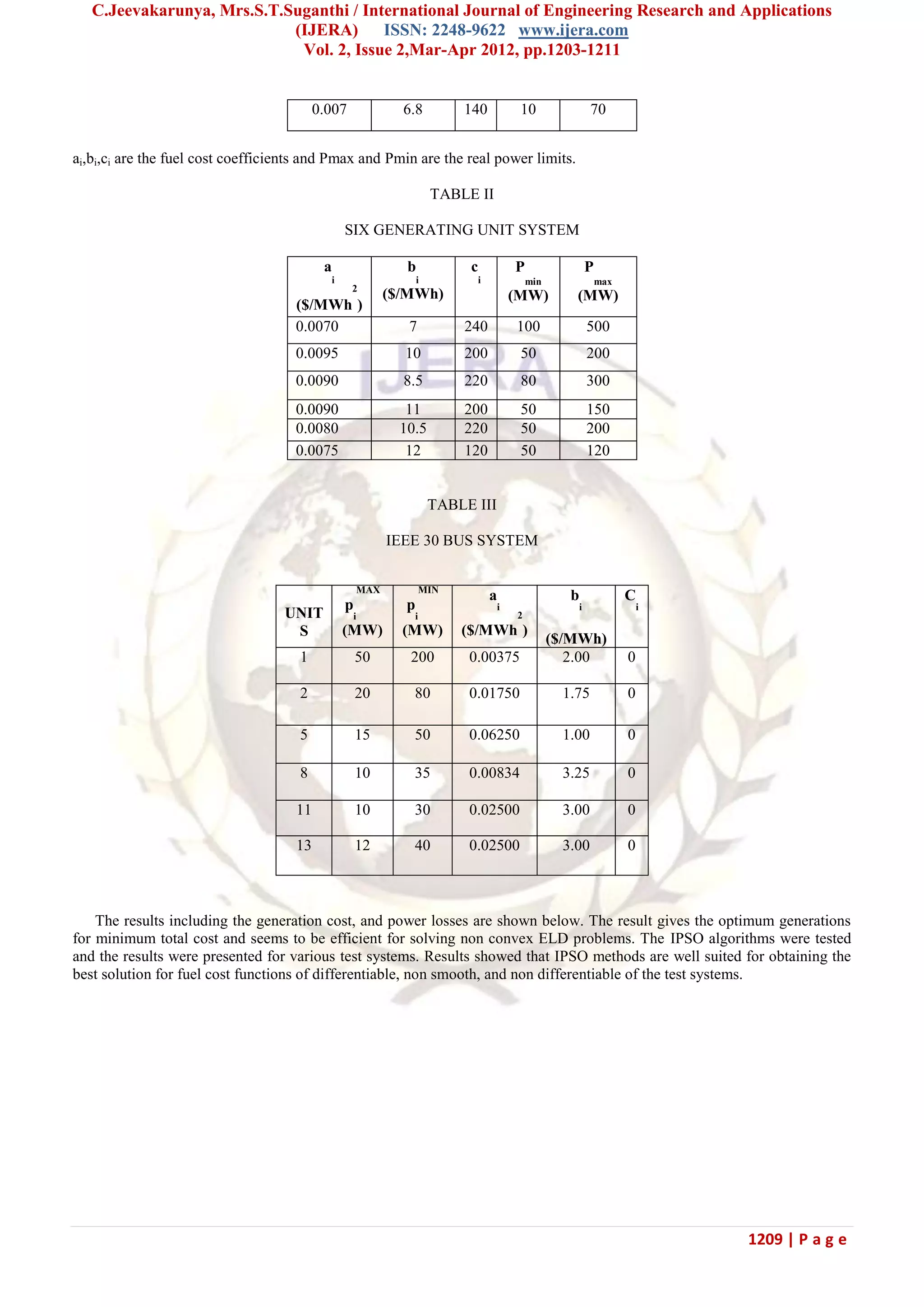
  C.Jeevakarunya, Mrs.S.T.Suganthi /International Journal of Engineering Research and Applications (IJERA) ISSN: 2248-9622 www.ijera.com Vol. 2, Issue 2,Mar-Apr 2012, pp.1203-1211 1210 | P a g e TABLE IV SIMULATION RESULT FOR THREE BUS SYSTEM TABLE V SIMULATION RESULT FOR SIX BUS SYSTEM IPSO PSO GA P1(MW) 323.6373 276.2339 277.322 P2(MW) 76.685 106.1268 105.2414 P3(MW) 158.435 143.868 144.5728 P4(MW) 50.00 54.5248 55.6876 P5(MW) 51.976 80.5364 82.7985 P6(MW) 50.00 50.00 51.000 Pl(MW) 10.73541 11.29094 11.6883 F($/hr) 8352.61 8388.13 8390.93 TABLE VI SIMULATION RESULT FOR IEEE 30 BUS SYSTEM 6. CONCLUSION In this paper, we have successfully employed the IPSO method to solve the ELD problem with the generator constraints. The IPSO algorithm has been demonstrated to have superior features, including high-quality solution, stable convergence characteristic, and good computation efficiency. Many nonlinear characteristics of the generator such as ramp rate limits, valve-point zones, and non smooth cost functions are considered for practical generator operation in the proposed method. The results show that the proposed method was indeed capable of obtaining higher quality solution efficiently in ED problems. REFERENCES [1] Bakirtzis, V. Petridis, and S. Kazarlis, ―Genetic algorithm solution to the economic dispatch problem,‖ Proc. Inst. Elect. Eng.–Gen., Transm.Dist., vol. 141, no. 4, pp. 377–382, July 1994. [2] F. N. Lee and A. M. Breipohl, ―Reserve constrained economic dispatch with prohibited operating zones,‖ IEEE Trans. Power Syst., vol. 8, pp.246–254, Feb. 1993. IPSO PSO GA P1(MW) 34.3249 32.8203 34.4895 P2(MW) 64.595 64.5435 64.0299 P3(MW) 54.9369 54.6427 54.1534 Pl(MW) 2.302049 2.540060 2.678 F($/hr) 1597.48 1597.72 1600 IPSO PSO GA P1(MW) 168.48 156.86 160.89 P2(MW) 46.47 49.984 50.984 P3(MW) 20.24 21.5873 22.7385 P4(MW) 182.279 184.627 185.627 P5(MW) 11.054 190.833 191.84 P6(MW) 277.59 255.44 256.44 P L (MW) 8.010 8.122 9.1 F($/hr) 796.51 801.085 803.08
• 9.
  C.Jeevakarunya, Mrs.S.T.Suganthi /International Journal of Engineering Research and Applications (IJERA) ISSN: 2248-9622 www.ijera.com Vol. 2, Issue 2,Mar-Apr 2012, pp.1203-1211 1211 | P a g e [3] C.-T. Su and G.-J. Chiou, ―A fast-computation hopfield method to economic dispatch of power systems,‖ IEEE Trans. Power Syst., vol. 12, pp.1759–1764, Nov. 1997. [4] T. Yalcinoz and M. J. Short, ―Neural networks approach for solving economic dispatch problem with transmission capacity constraints,‖ IEEE Trans. Power Syst., vol. 13, pp. 307–313, May 1998. [5] D. C.Walters and G. B. Sheble, ―Genetic algorithm solution of economic dispatch with valve point loading,‖ IEEE Trans. Power Syst., vol. 8, pp.1325–1332, Aug. 1993. [6] K. P. Wong and Y. W. Wong, ―Genetic and genetic/simulated — Annealing approaches to economic dispatch,‖ Proc. Inst. Elect. Eng., pt. C,vol. 141, no. 5, pp. 507–513, Sept. 1994. [7] G. B. Sheble and K. Brittig, ―Refined genetic algorithm — Economic dispatch example,‖ IEEE Trans. Power Syst., vol. 10, pp. 117–124, Feb.1995. [8] P.-H. Chen and H.-C. Chang, ―Large-Scale economic dispatch by genetic algorithm,‖ IEEE Trans. Power Syst., vol. 10, pp. 1919–1926, Nov.1995. [9] C. C. Fung, S. Y. Chow, and K. P. Wong, ―Solving the economic dispatch problem with an integrated parallel genetic algorithm,‖ in Proc. Power Con Int. Conf., vol. 3, 2000, pp. 1257–1262. [10] T. Yalcionoz, H. Altun, and M. Uzam, ―Economic dispatch solution using a genetic algorithm based on arithmetic crossover,‖ in Proc. IEEE Proto Power Tech. Conf., Proto, Portugal, Sept. 2001. [11] D. B. Fogel, Evolutionary Computation: Toward a New Philosophy of Machine Intelligence, 2 ed. Piscataway, NJ: IEEE Press, 2000. [12] K. S. Swarup and S. Yamashiro, ―Unit commitment solution methodology using genetic algorithm,‖ IEEE Trans. Power Syst., vol. 17, pp.87–91, Feb. 2002. [13] J. Kennedy and R. Eberhart, ―Particle swarm optimization,‖ Proc. IEEE Int. Conf. Neural Networks, vol. IV, pp. 1942–1948, 1995. [14] Y. Shi and R. Eberhart, ―A modified particle swarm optimizer,‖ Proc.IEEE Int. Conf. Evol. Comput., pp. 69–73, May 1998. [15] Y. Shi and R. C. Eberhart, ―Empirical study of particle swarm optimization,‖ in Proc. Congr. Evol. Comput., NJ, 1999, pp. 1945–1950. [16] R. C. Eberhart and Y. Shi, ―Comparison between genetic algorithms and particle swarm optimization,‖ Proc. IEEE Int. Conf. Evol. Comput., pp.611–616, May 1998. [17] P. J. Angeline, ―Using selection to improve particle swarm optimization,‖Proc. IEEE Int. Conf. Evol. Comput., pp. 84–89, May 1998. [18] H. Yoshida, K. Kawata, Y. Fukuyama, S. Takayama, and Y. Nakanishi,―A particle swarm optimization for reactive power and voltage control considering voltage security assessment,‖ IEEE Trans. Power Syst., vol.15, pp. 1232– 1239, Nov. 2000. [19] S. Naka, T. Genji, T. Yura, and Y. Fukuyama, ―Practical distribution state estimation using hybrid particle swarm optimization,‖ Proc. IEEE Power Eng. Soc. Winter Meeting, vol. 2, pp. 815–820, 2001. [20] H. Saadat, Power System Analysis. New York: McGraw-Hill, 1999.