Downloaded 204 times
![Brown Level Optimisation private GetBytes getBytesCache; public byte[] getBytes(String charsetName) throws UnsupportedEncodingException { if (charsetName == null) throw new NullPointerException(); GetBytes getBytes = getBytesCache; if (getBytes != null && getBytes.charsetName.equals(charsetNam e))](https://image.slidesharecdn.com/gc-freecoding-140515092303-phpapp02/75/GC-free-coding-in-Java-presented-Geecon-22-2048.jpg)


The document discusses optimizing Java applications for low garbage collection (GC) and low latency in high-frequency trading (HFT) environments, highlighting the importance of memory utilization and CPU cache efficiency. It introduces key open-source projects and techniques for minimizing pauses, using primitives, and the efficient management of data through optimized data structures. Additionally, it covers strategies for building low-latency systems, critical path databases, and the use of specialized tools like Java Chronicle for high-throughput logging.
An introduction by Peter Lawrey about GC Free coding, agenda of the talk, and who Higher Frequency Trading is.
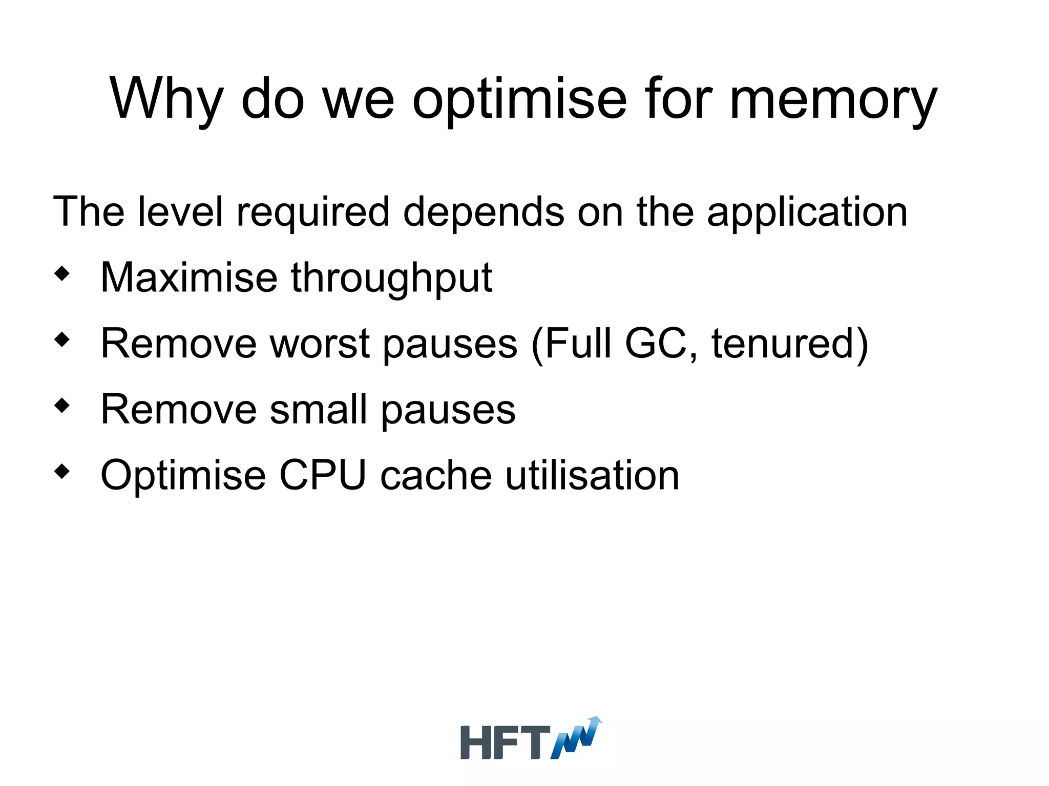
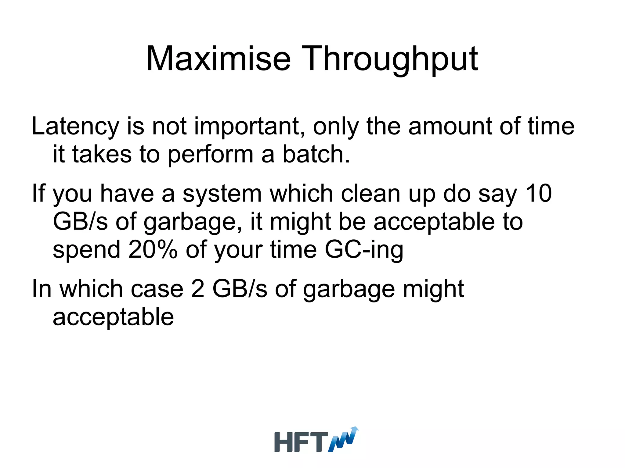
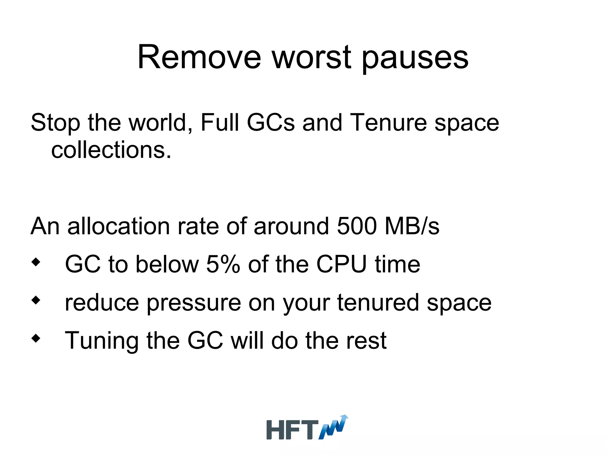
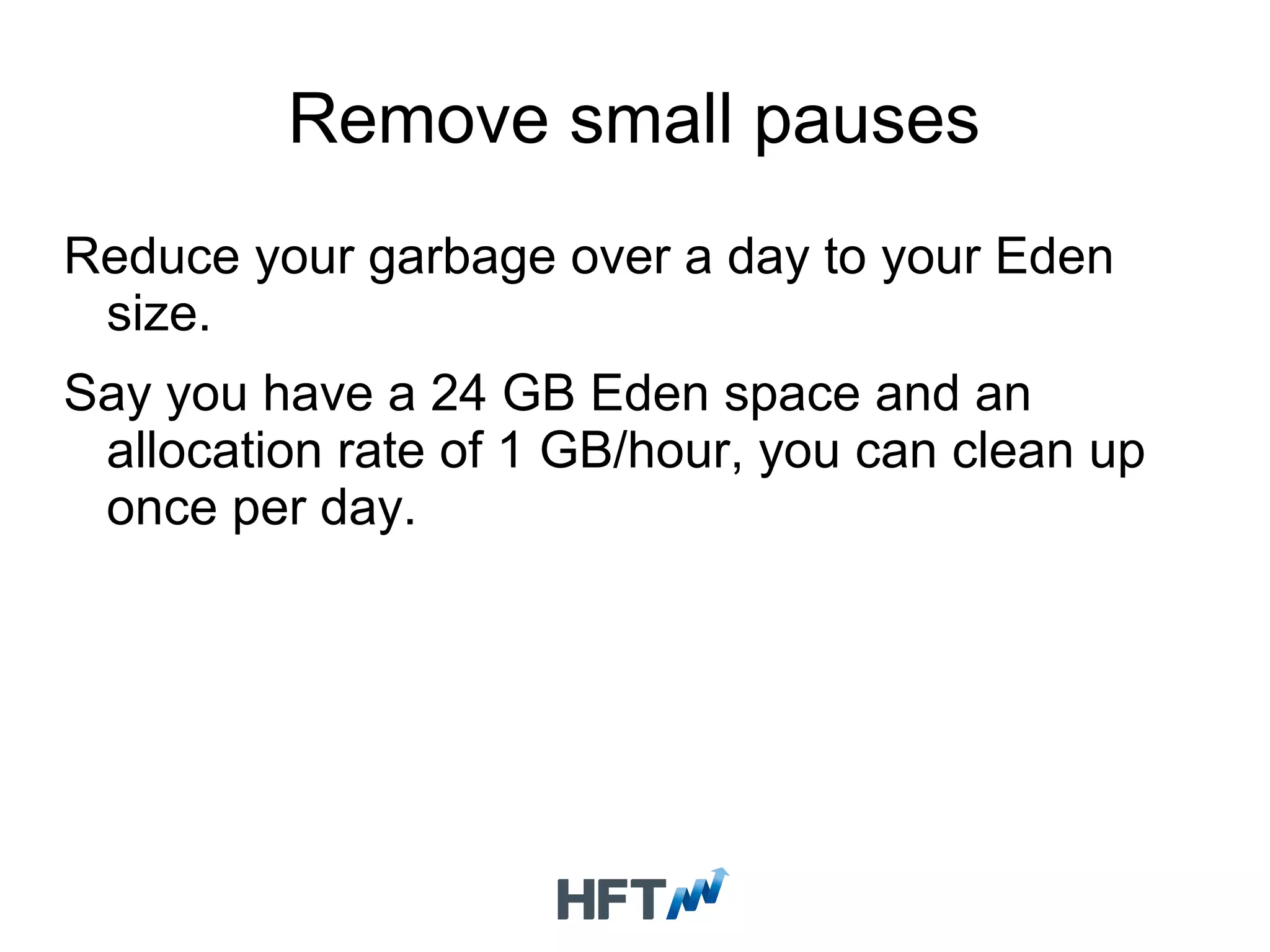
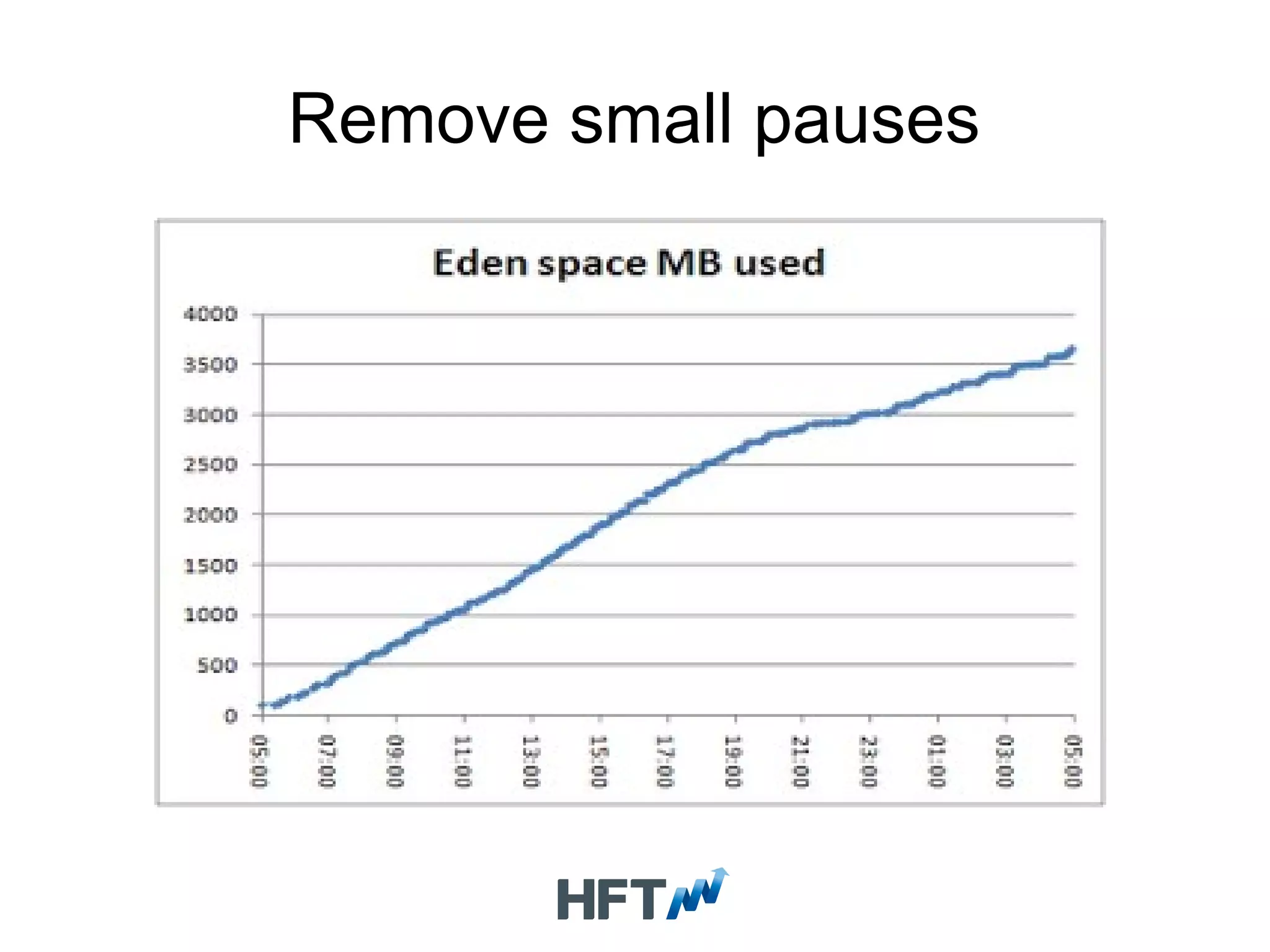
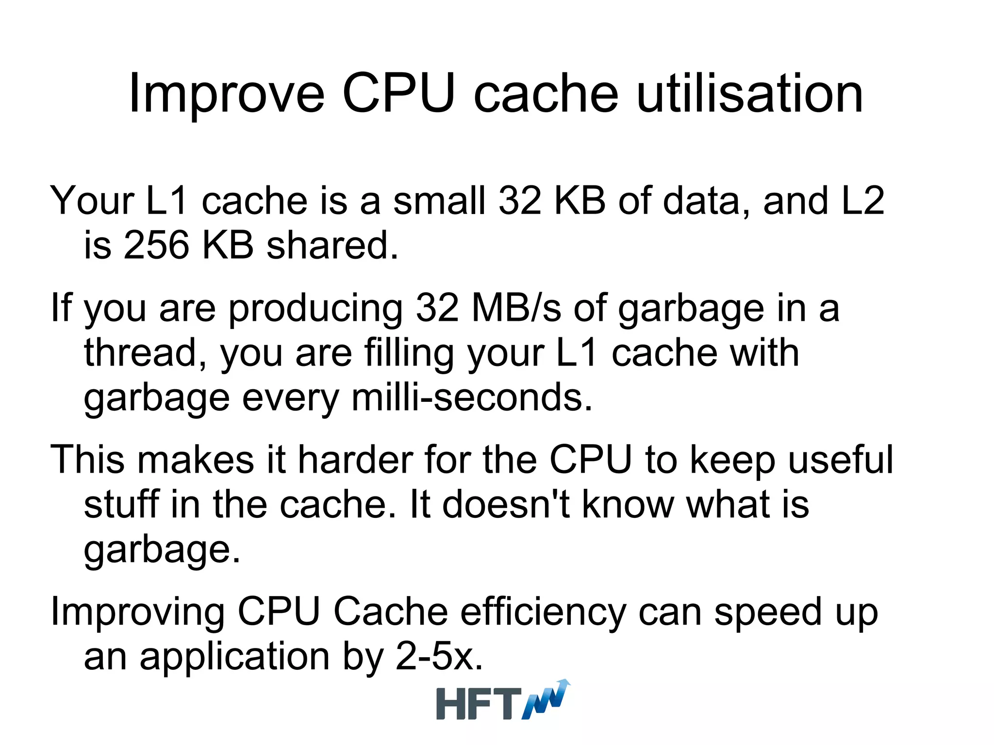
Discusses the importance of memory optimization, focusing on maximizing throughput, removing pauses, and improving CPU cache utilization.
Explains when to optimize code, emphasizing the significance of proper testing and evaluation before optimization.
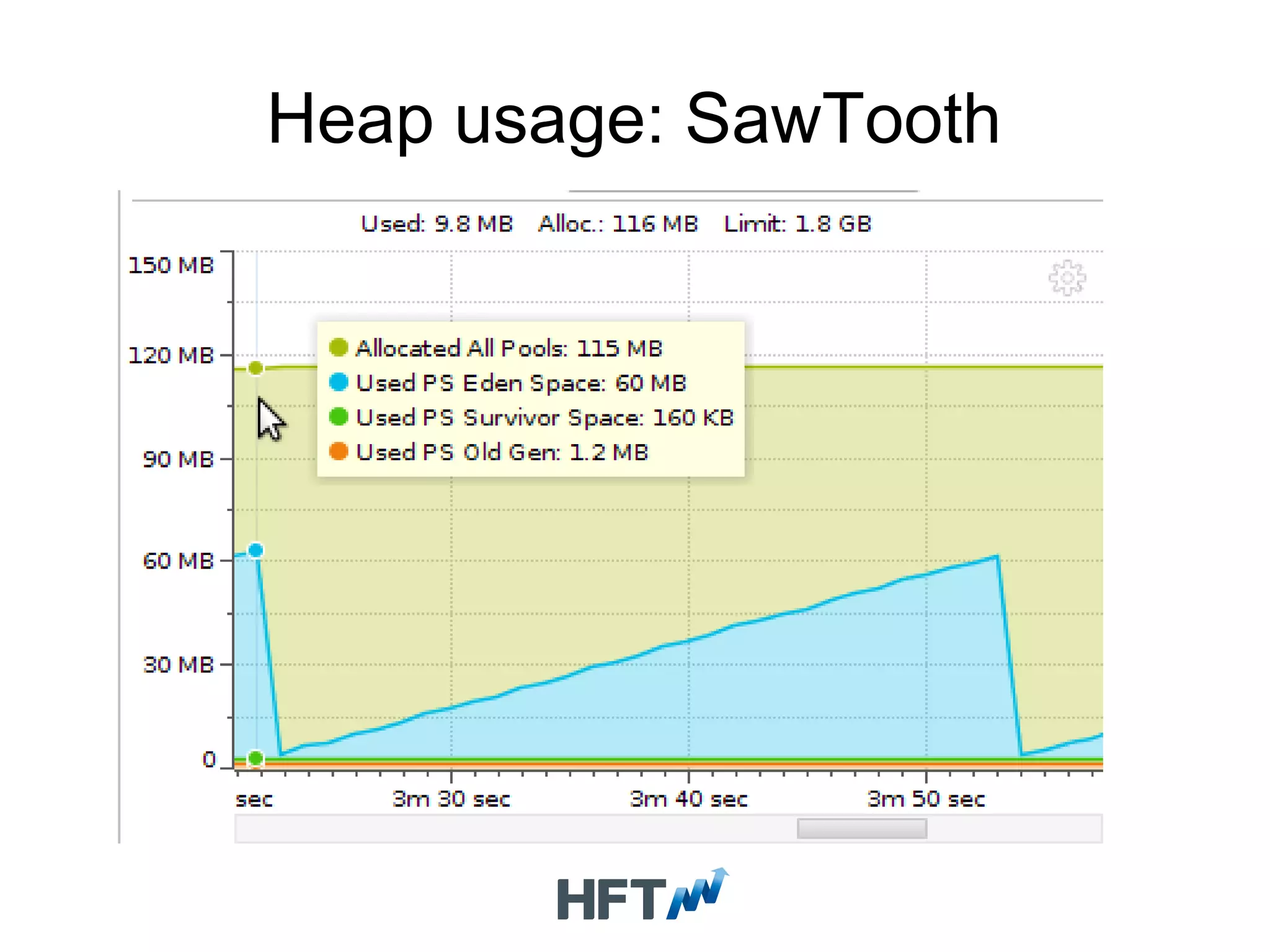
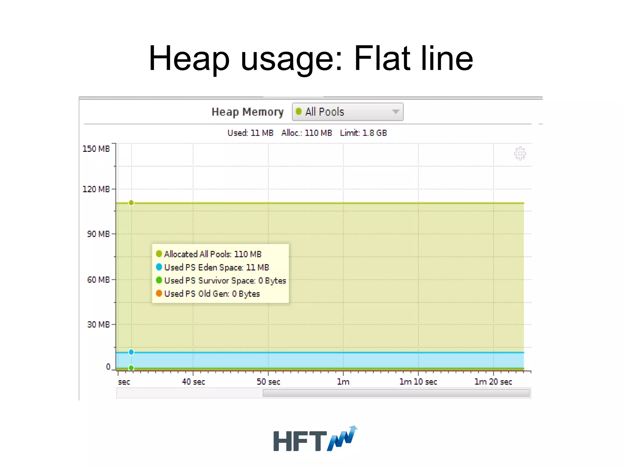
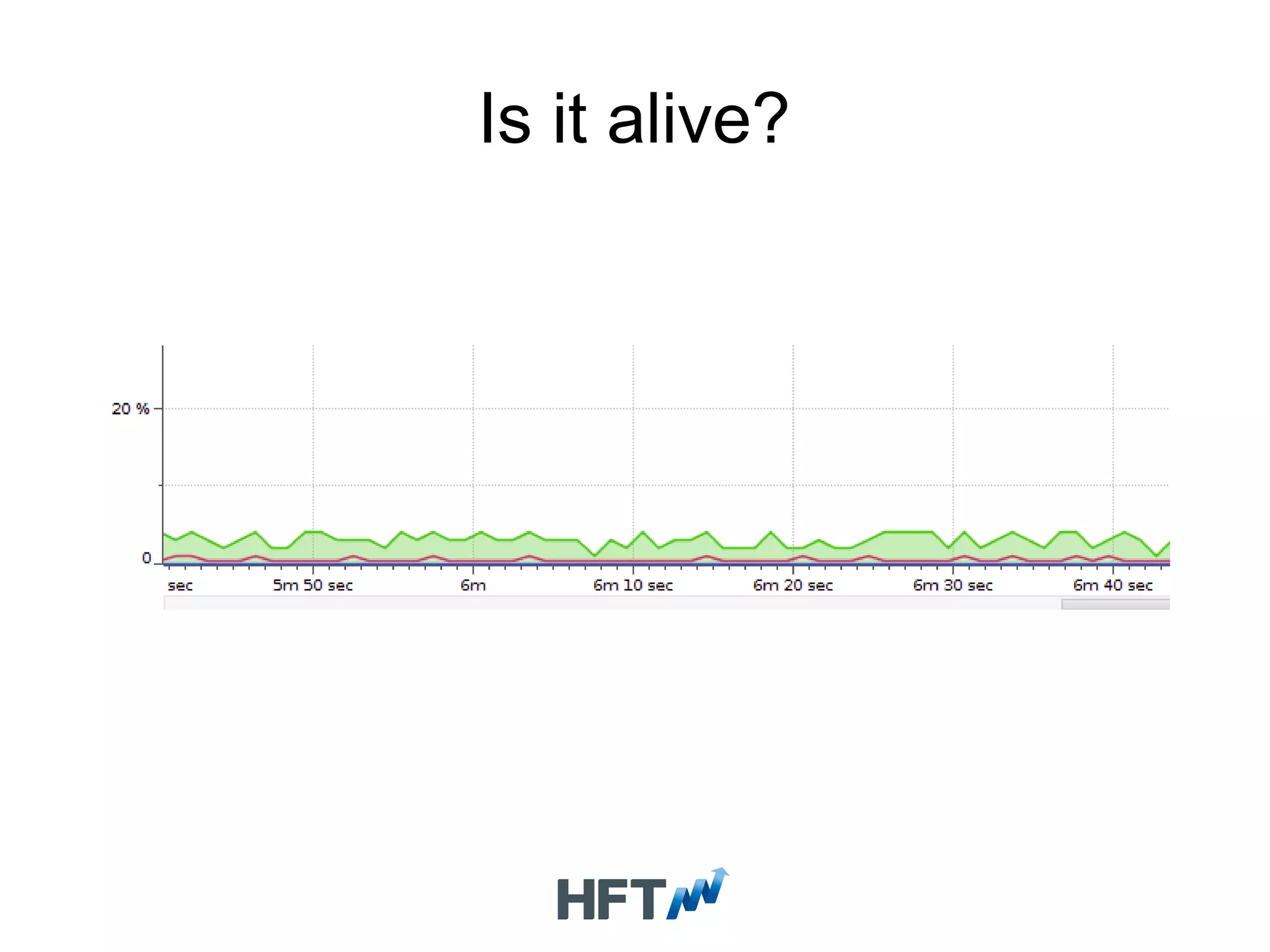
Guidelines for profiling applications, initiating optimization processes using correct test cases, and monitoring heap usage.
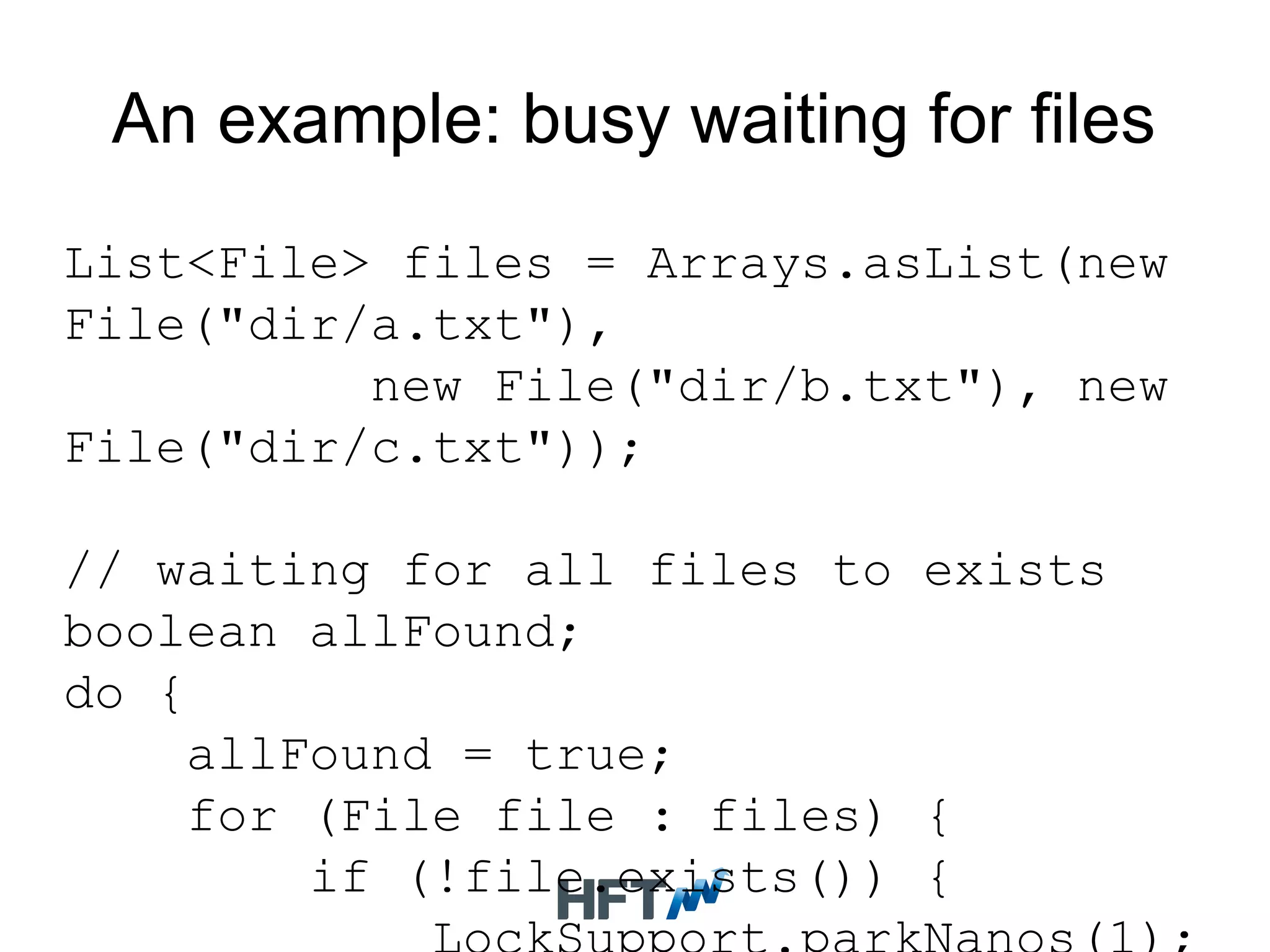
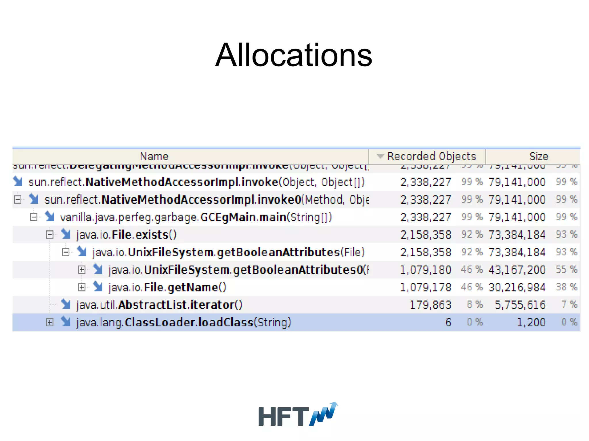
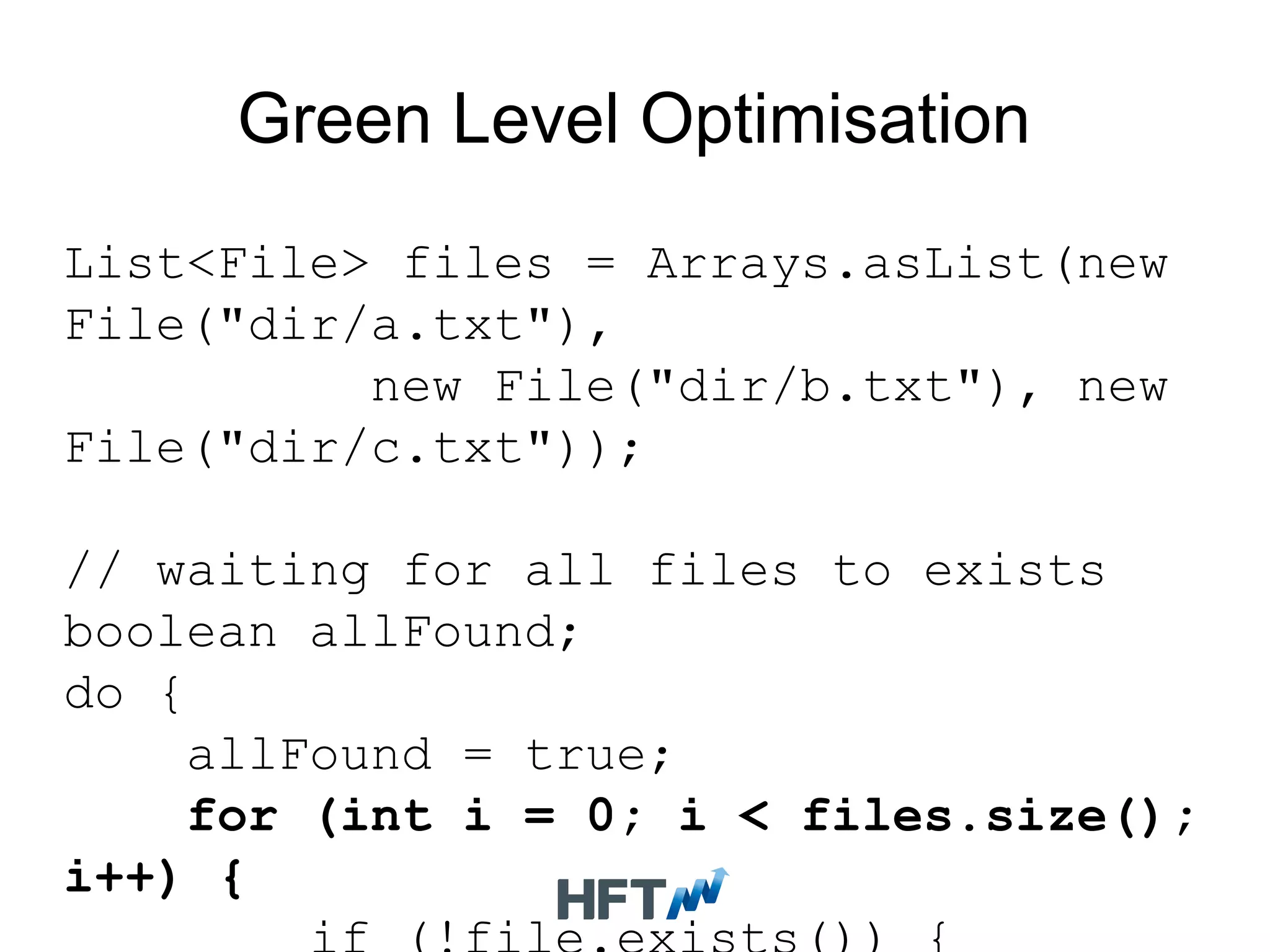
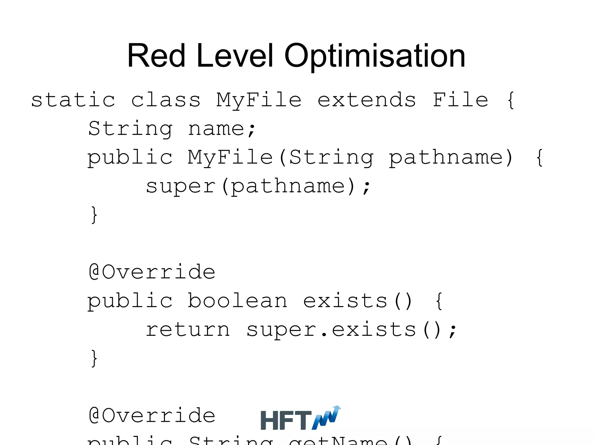
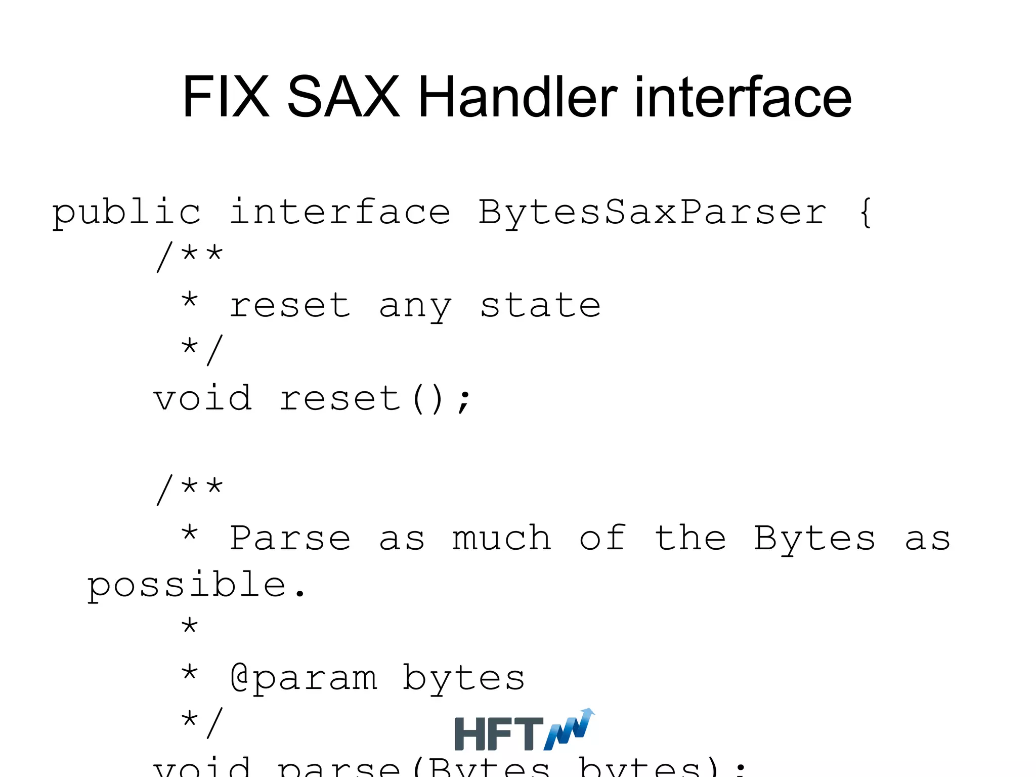
Demonstrates various levels of code optimization through practical examples of file handling improvements.
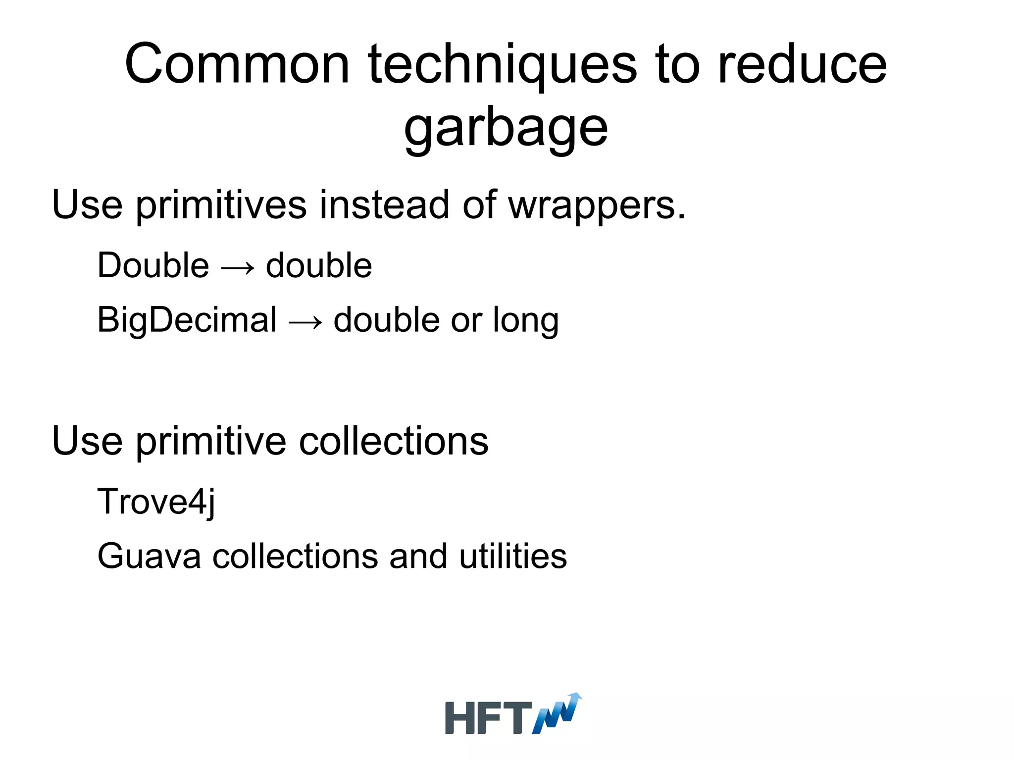
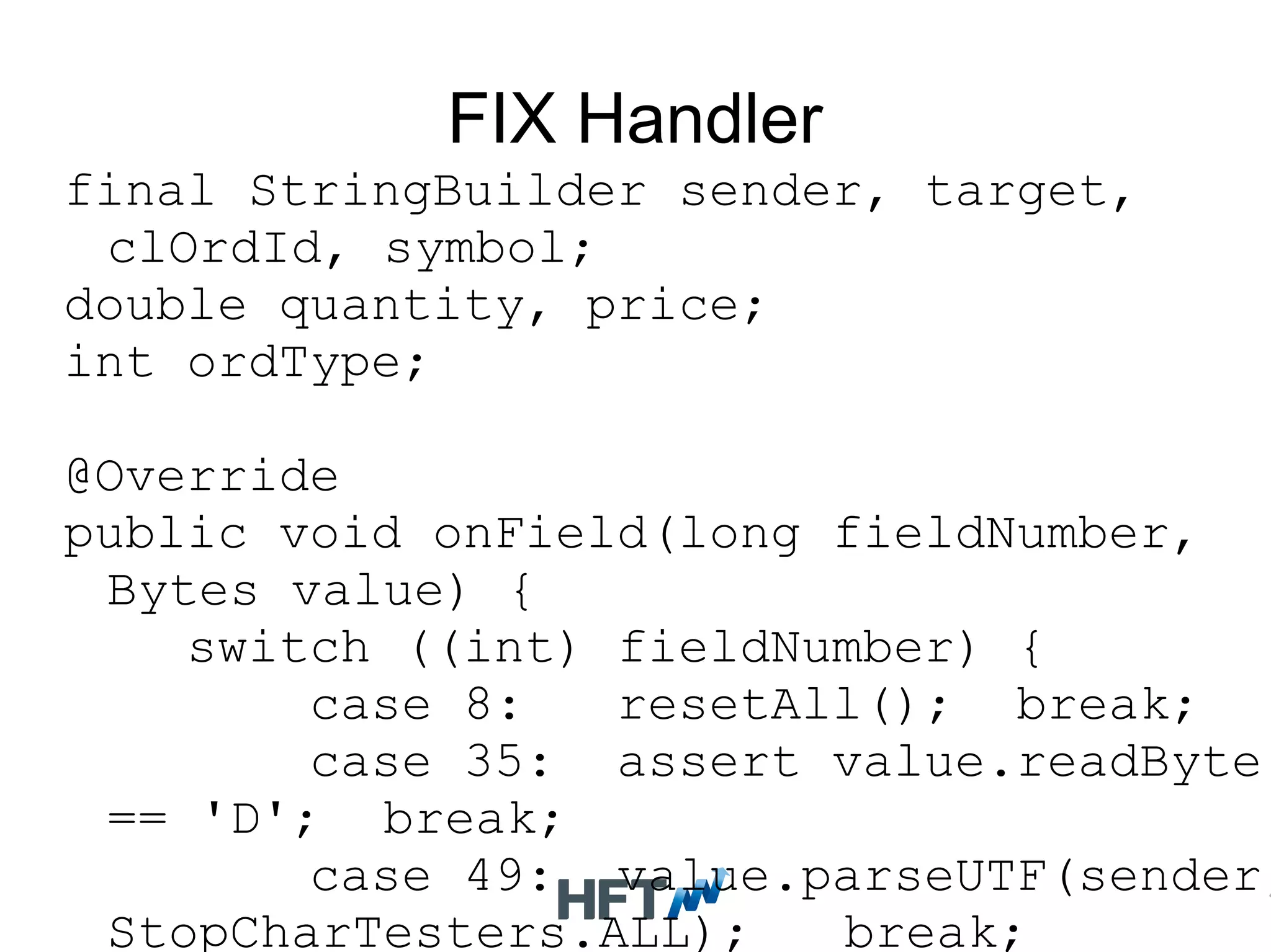
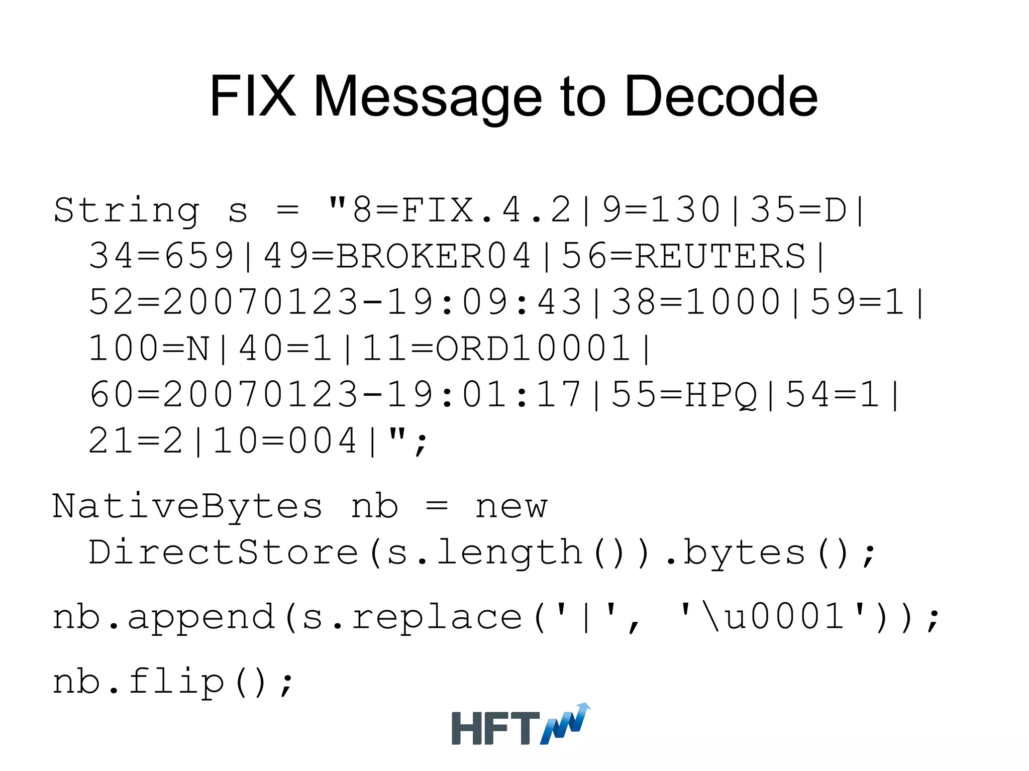
Outlines techniques to reduce garbage collection overhead like using primitives over wrappers and SAX instead of DOM.
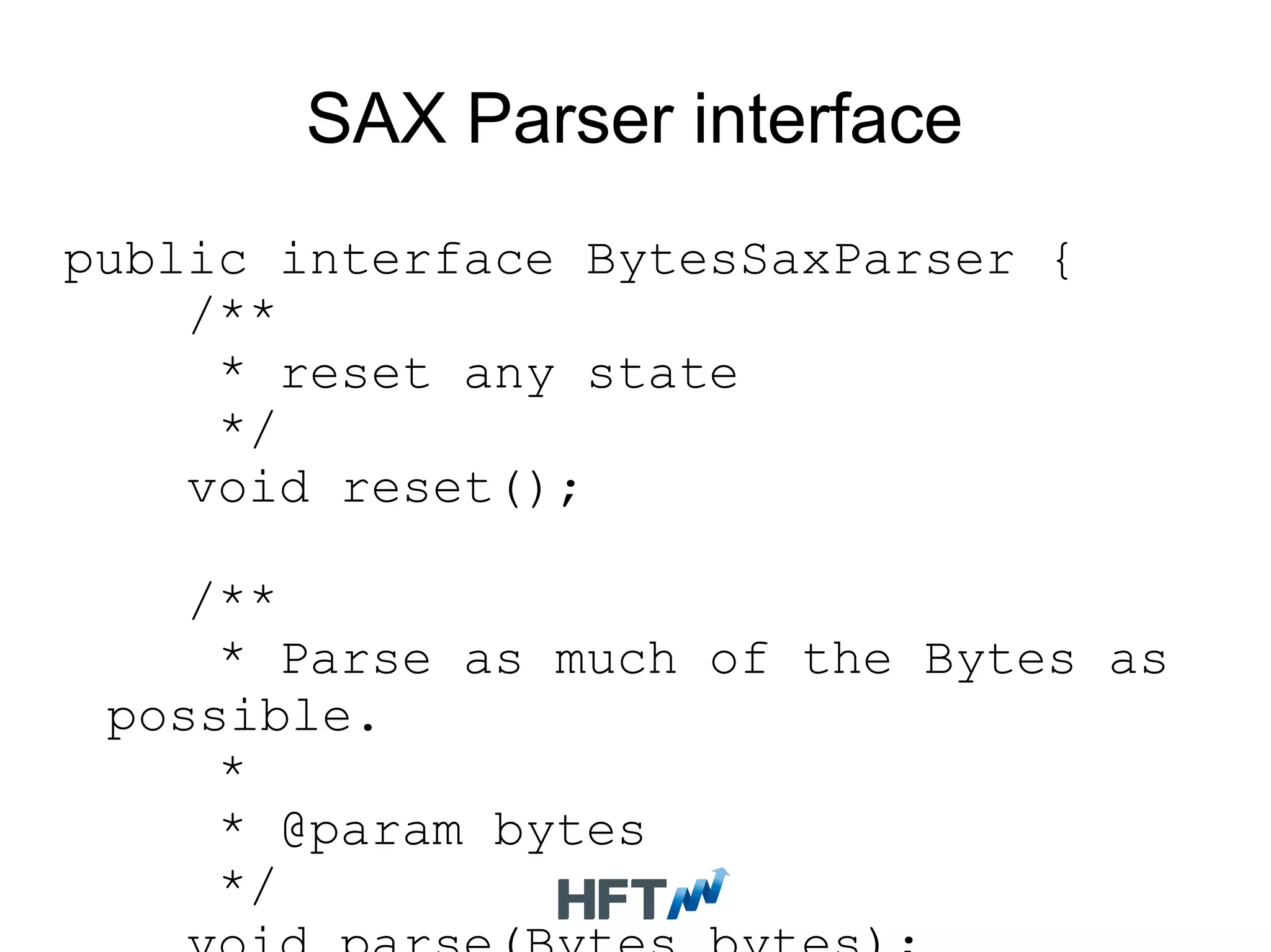
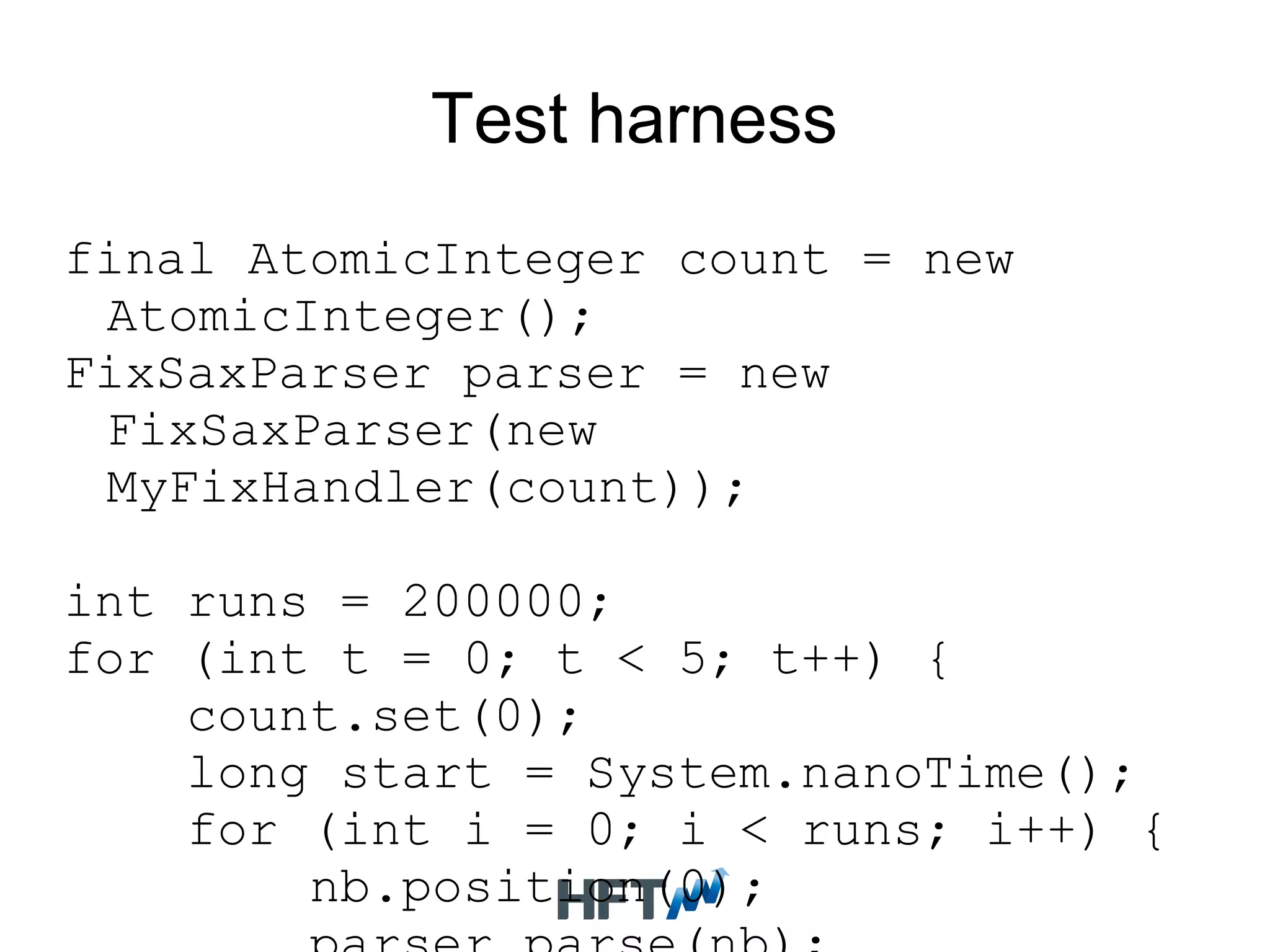
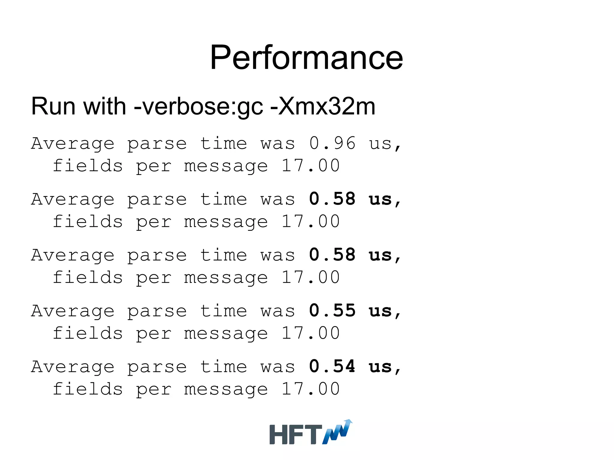
Introduction and performance metrics for SAXophone, discussing its GC-free features and efficiency in processing.
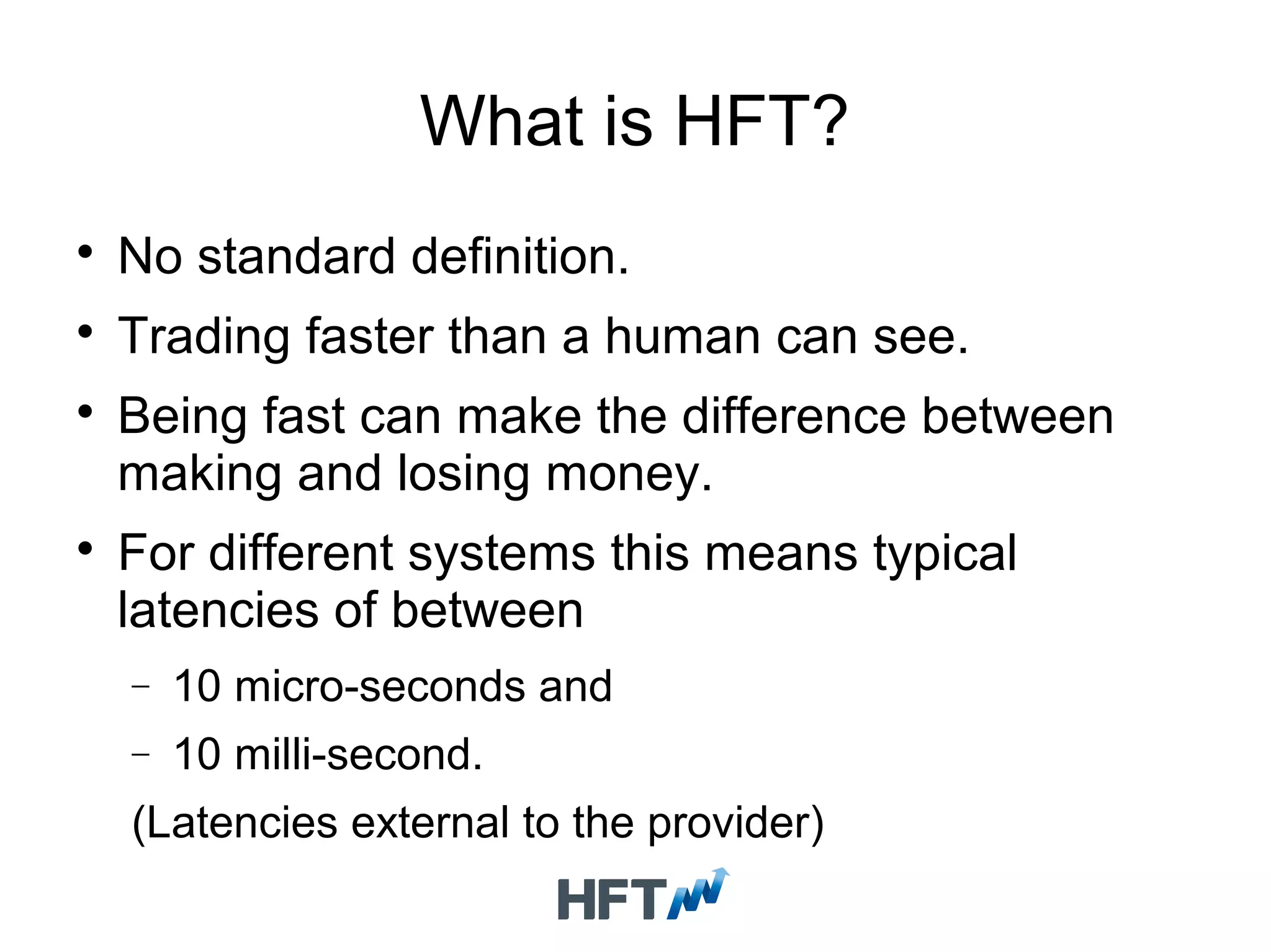
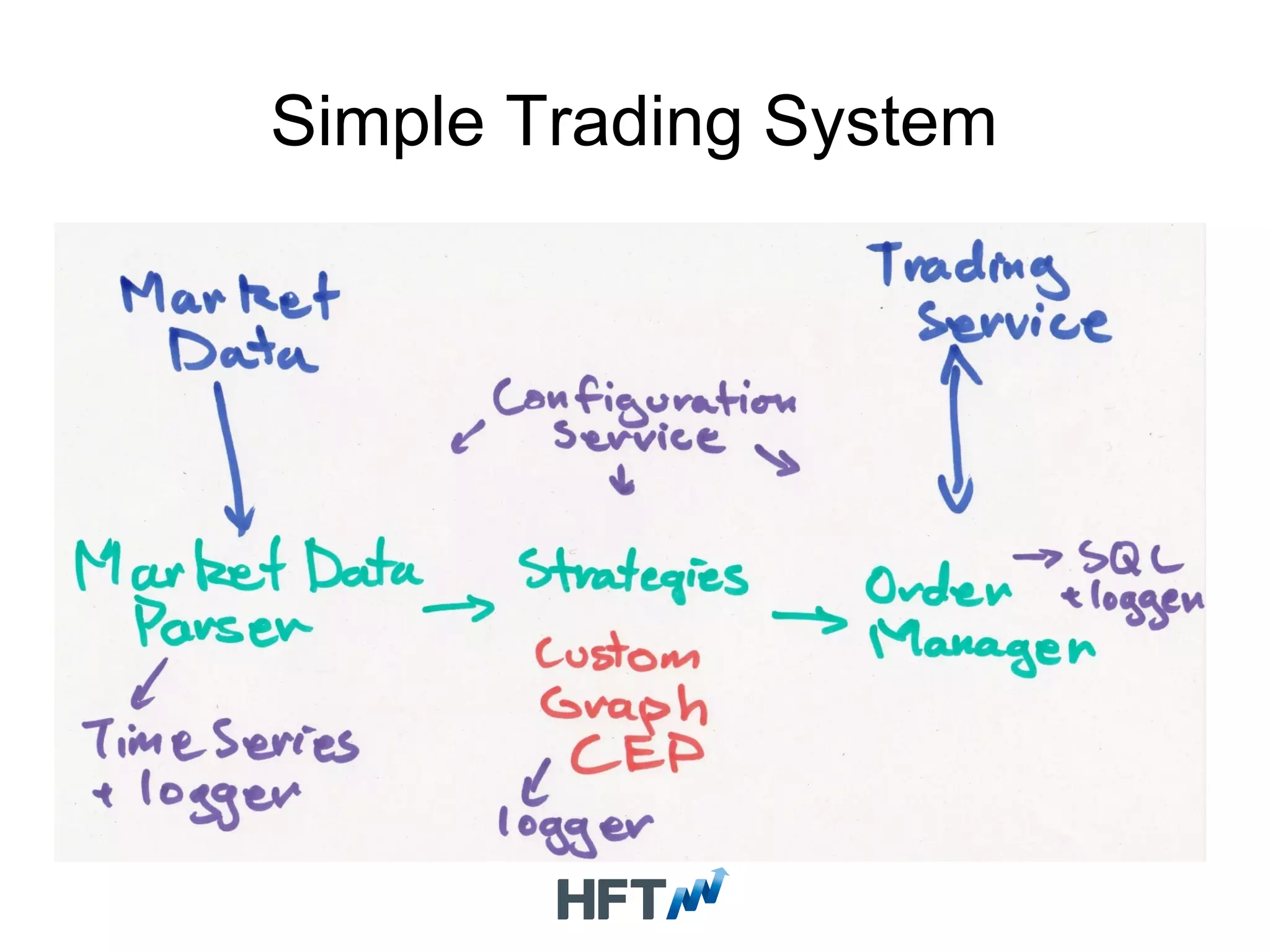
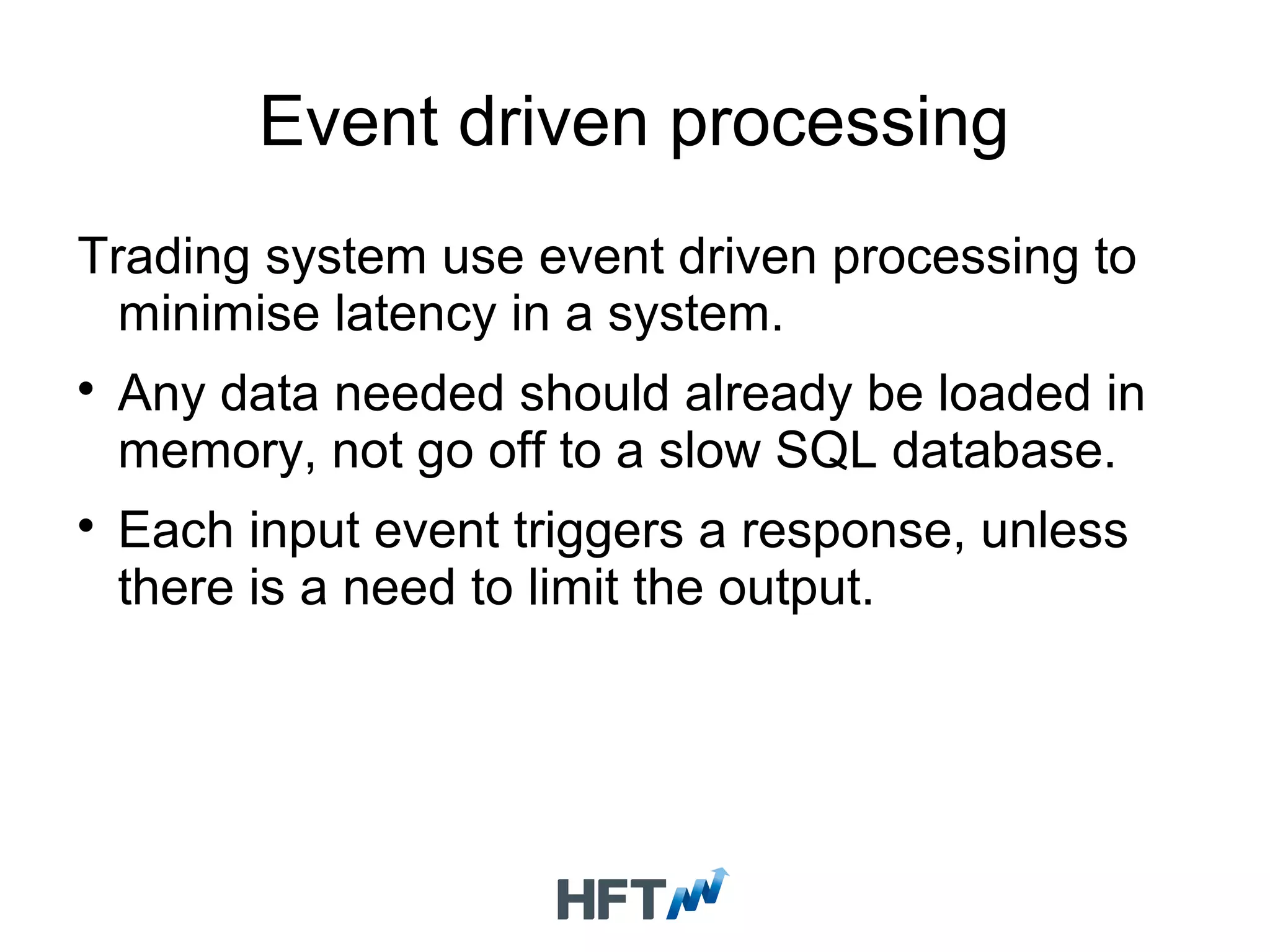
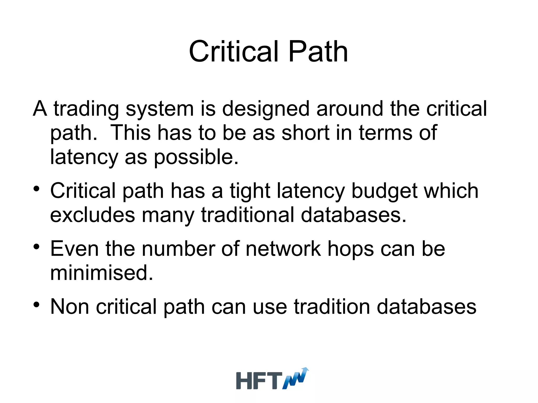
Defines HFT, discusses the importance of minimizing latency, and outlines critical paths in trading systems.
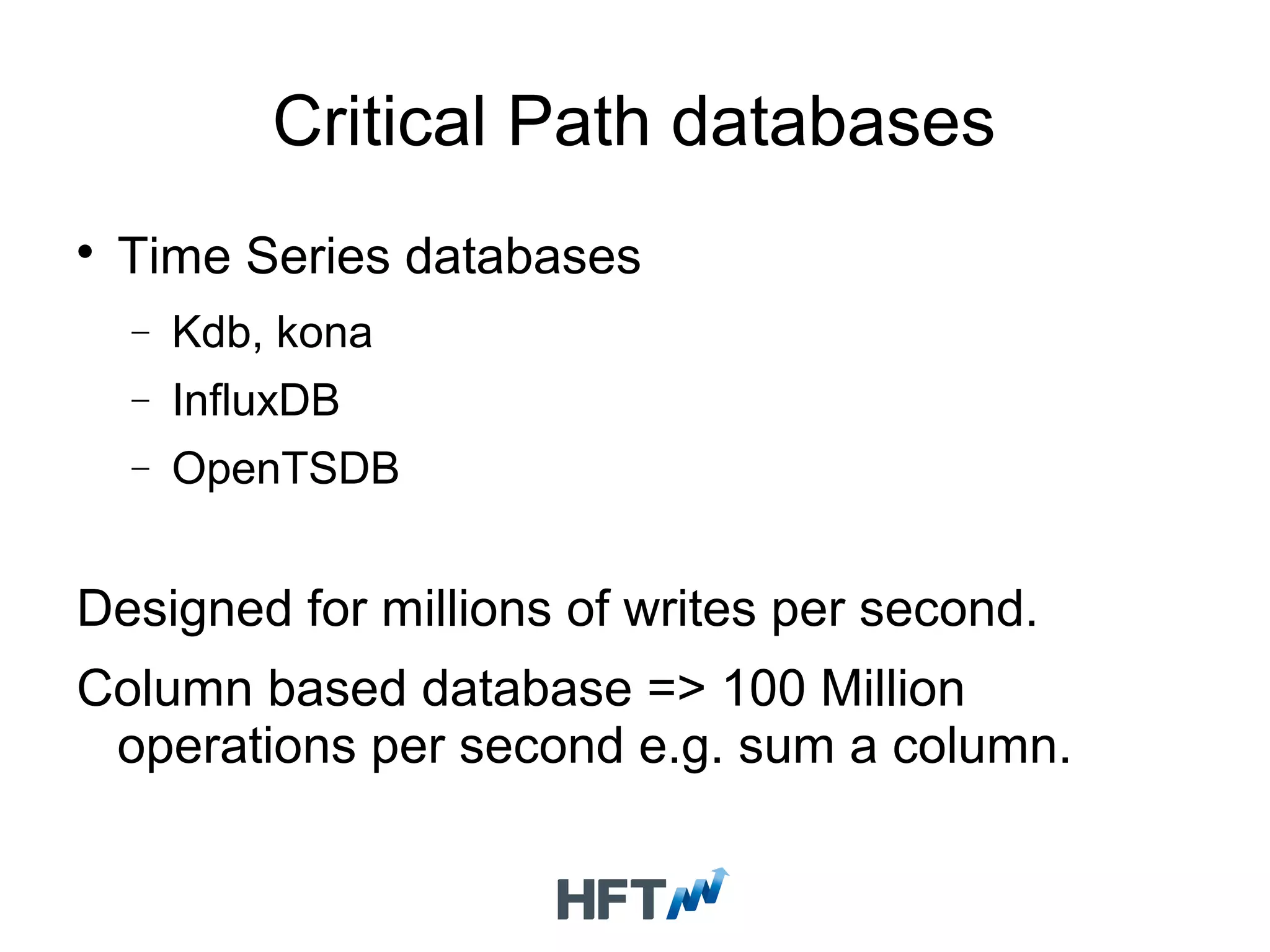
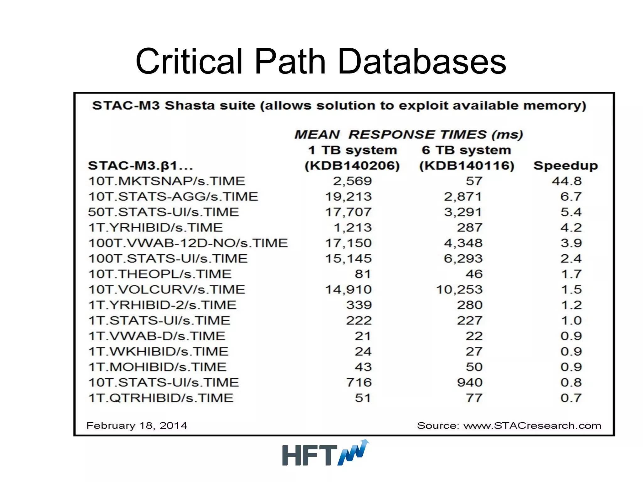
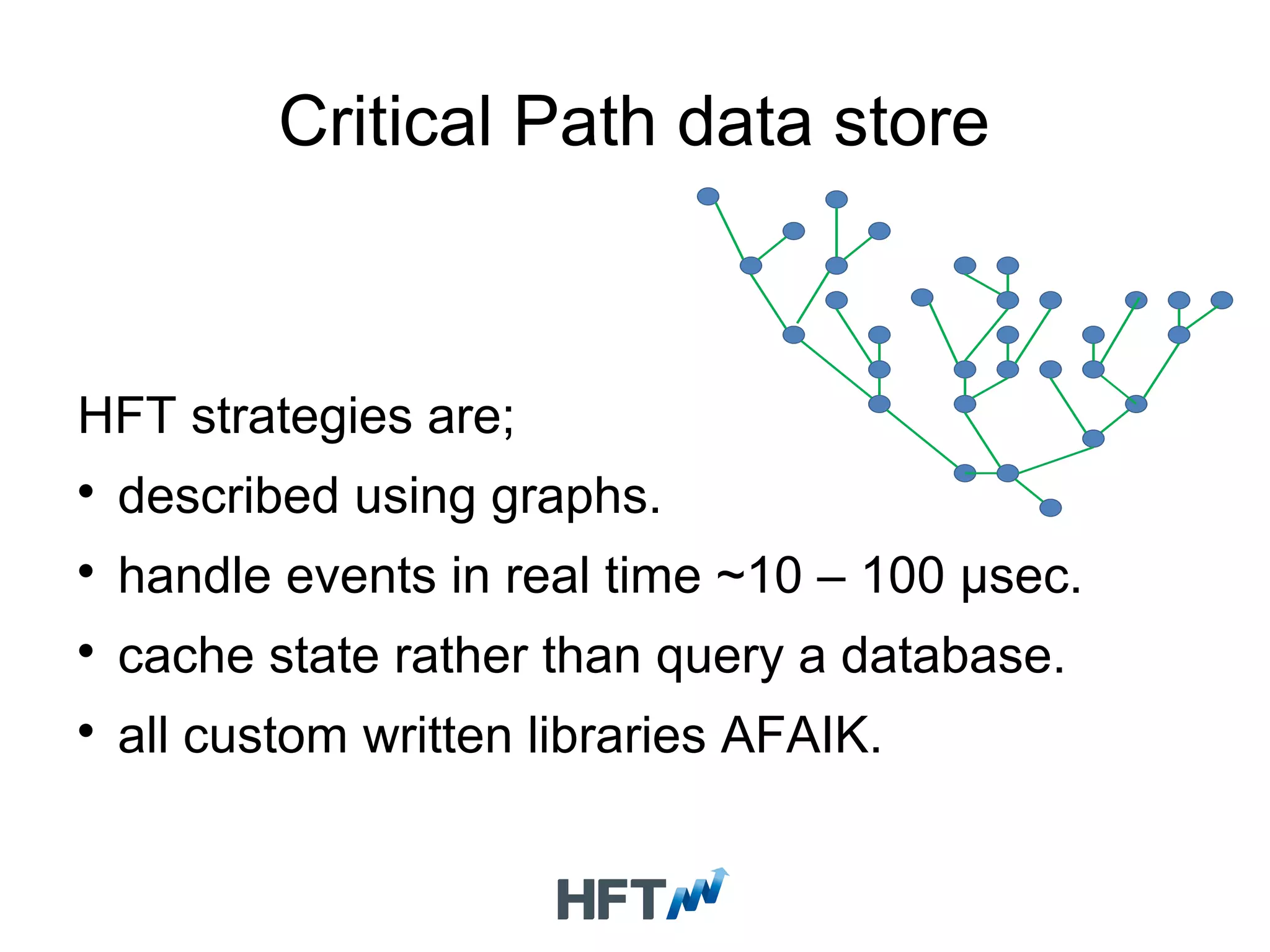
Overview of suitable databases for HFT applications with emphasis on high throughput and low latency.
Describes control, management infrastructure, and the benefits of specialized databases in HFT environments.
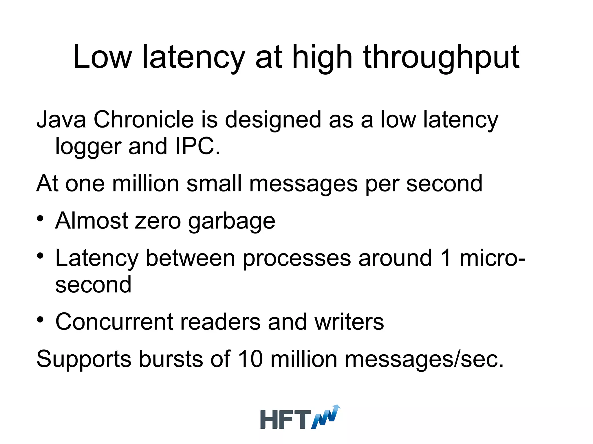
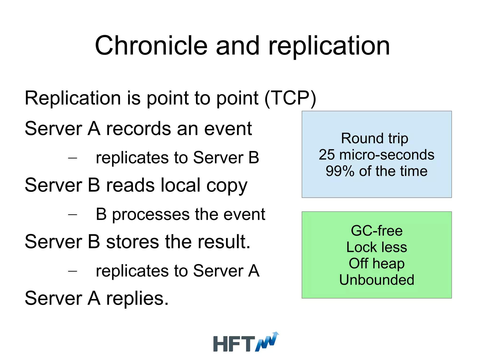
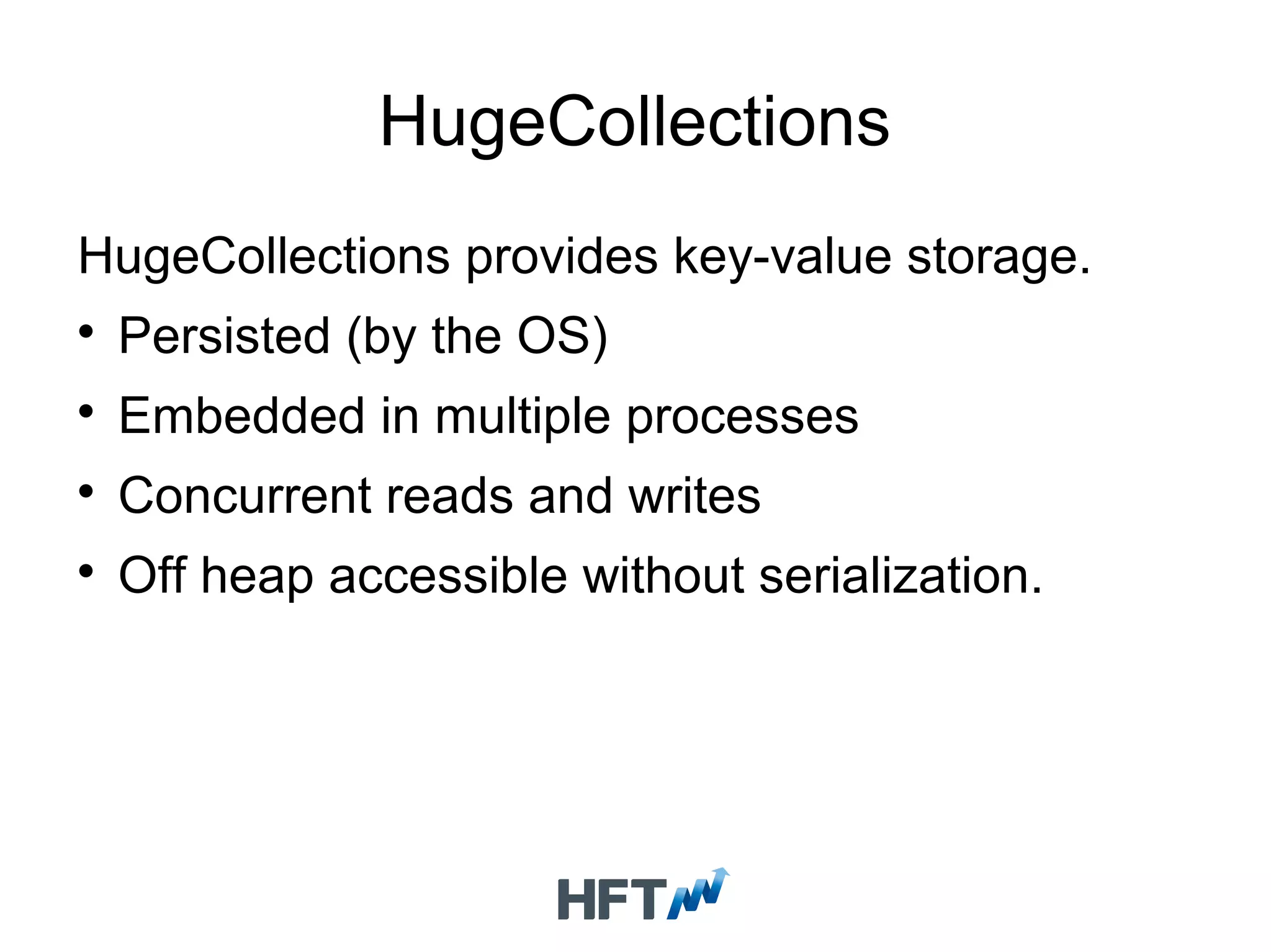
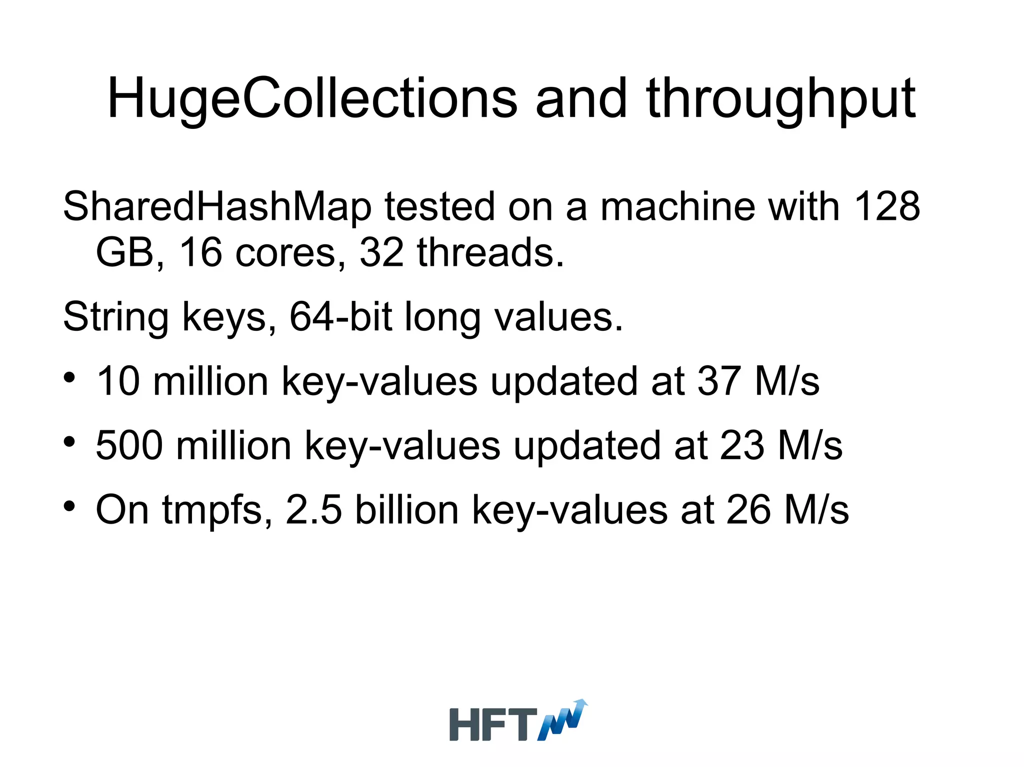
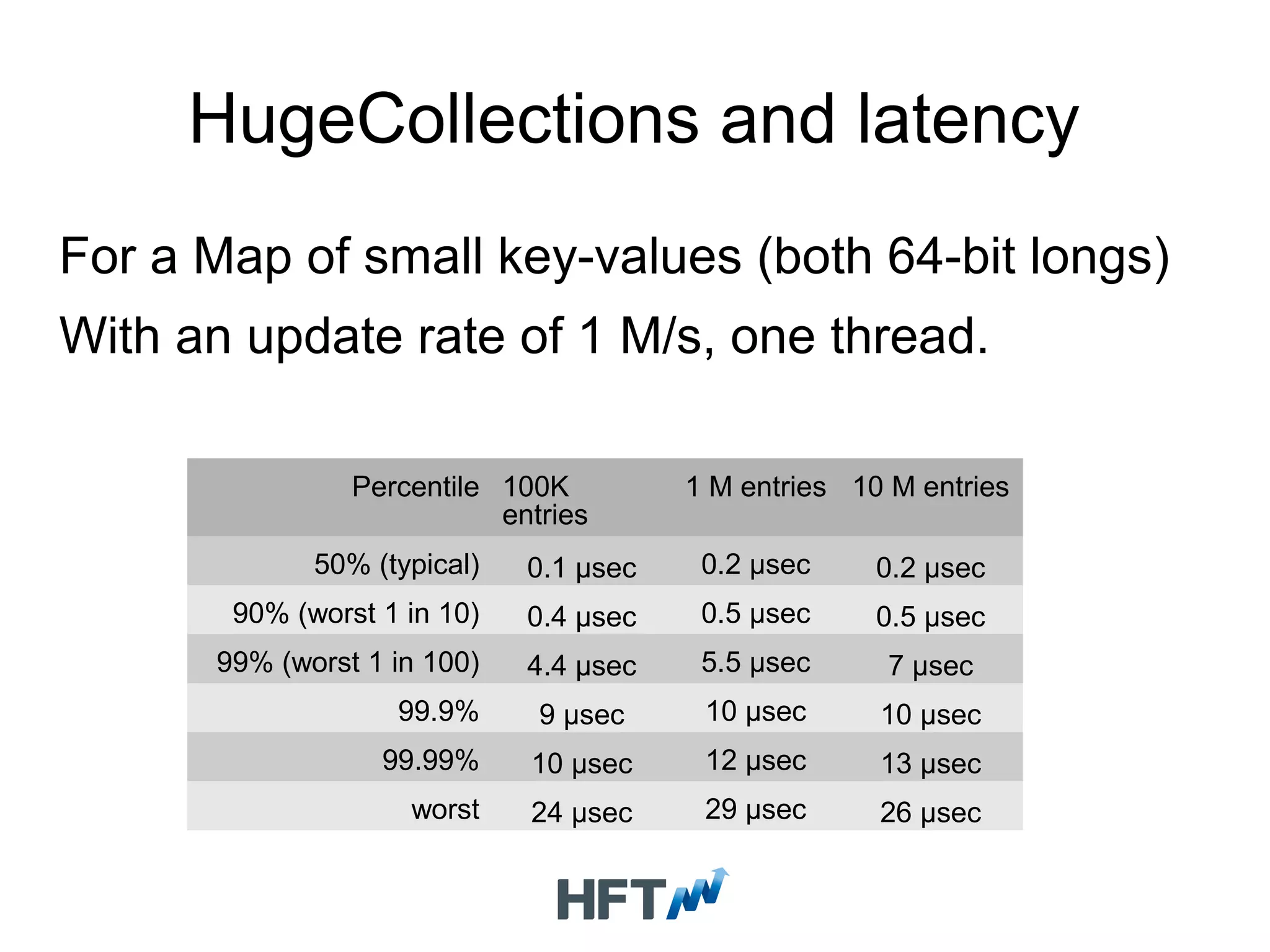
Details on Java Chronicle as a low-latency logger and performance results of HugeCollections in storage tasks.
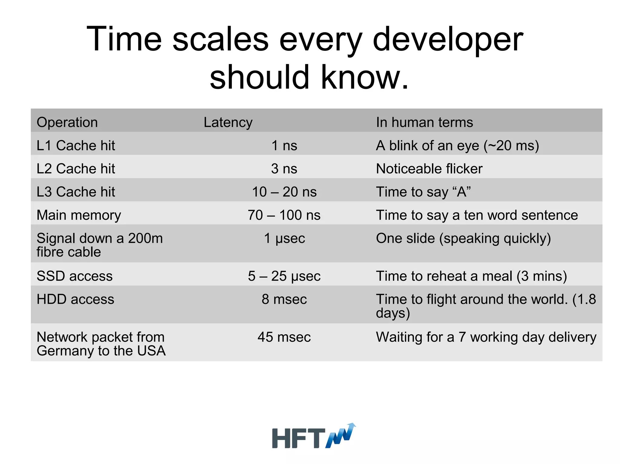
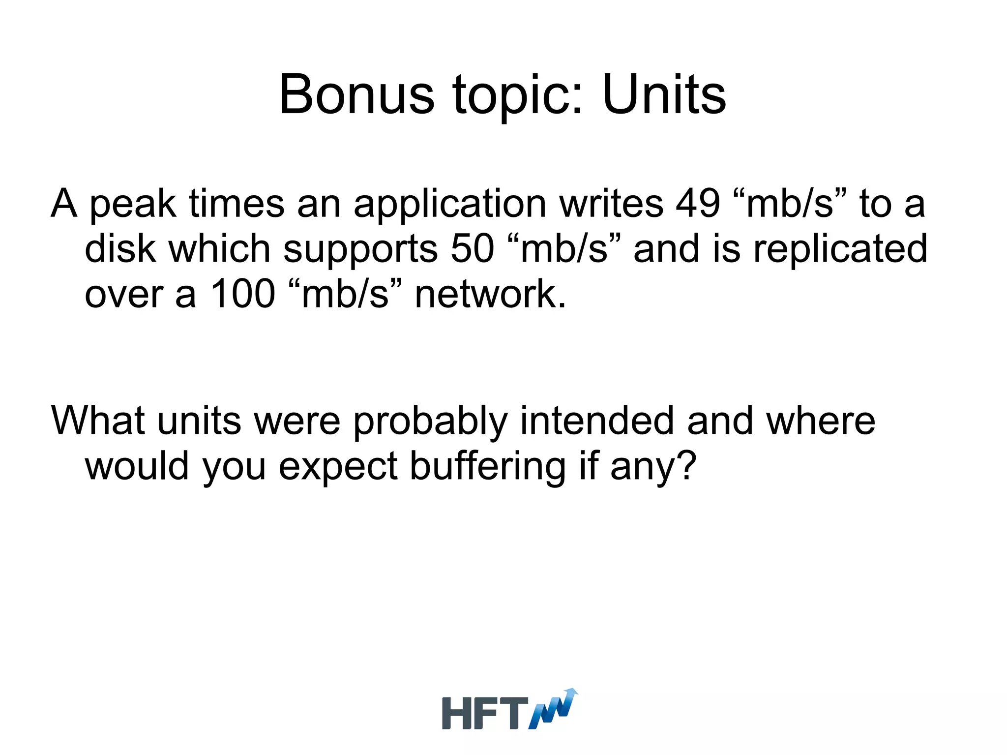
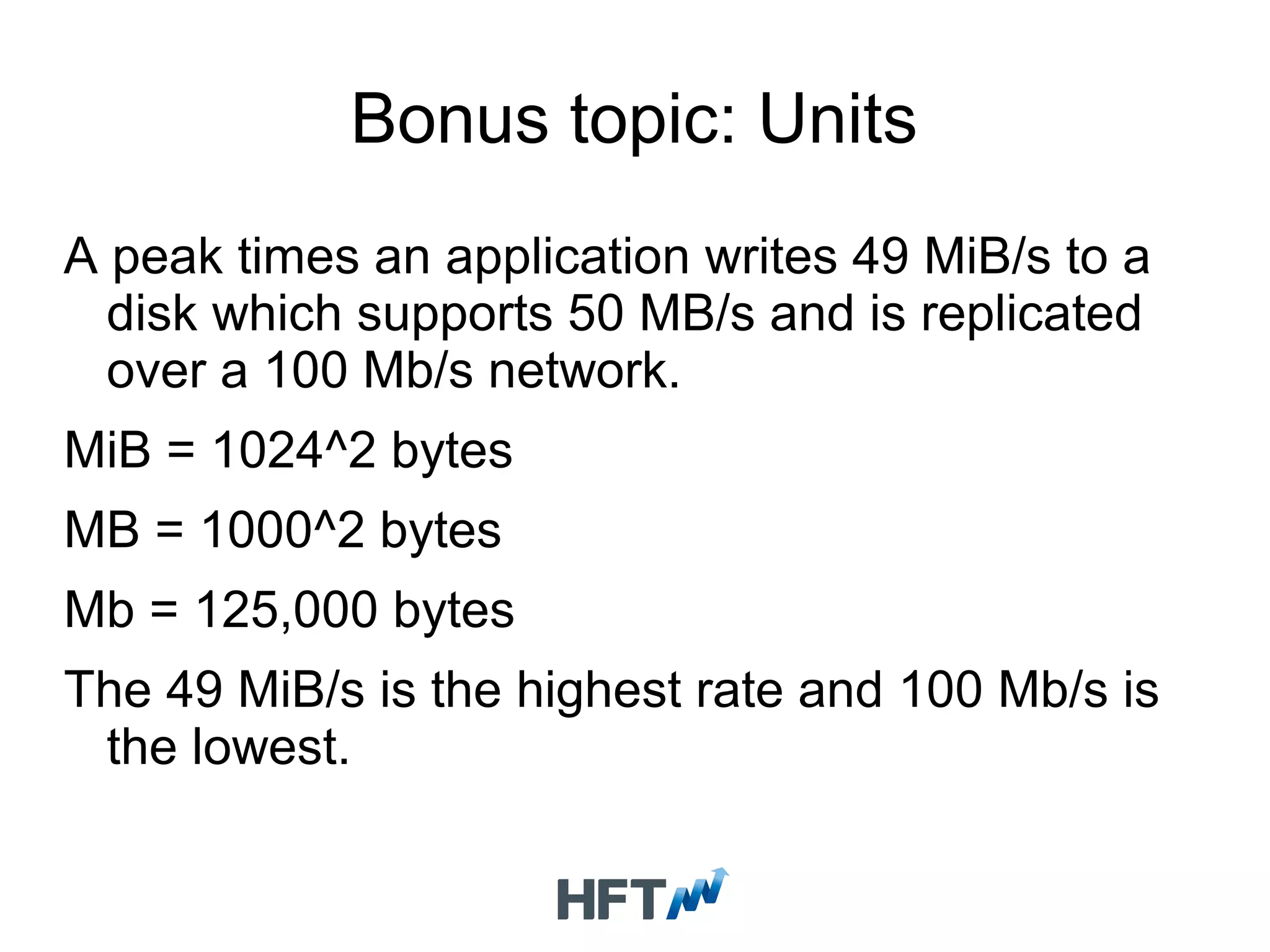
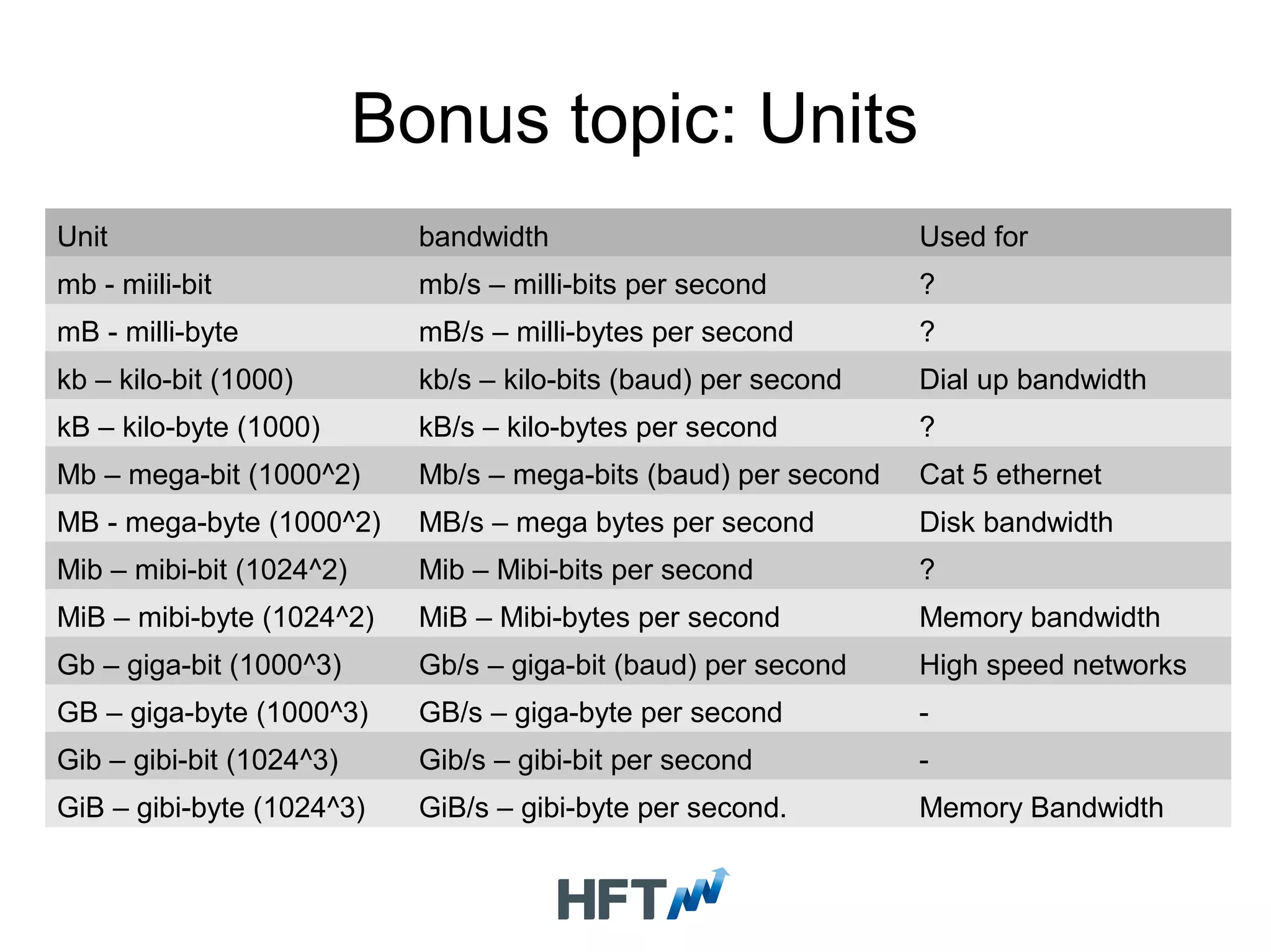
Explains different units of measurements and their significance in bandwidth discussions related to performance.