Data Structure and Algorithms (DSA) with Python

A Training report on “DSA with Python” submitted in partial fulfilment for the award of the Degree of Bachelor of Technology In Department of Computer Science & Engineering (With specialisation in Computer Science & Engineering) Submitted By: Student Name Roll No.: 22EJExxxxxx Submitted To: Mr. Prof. Name (HOD of CSE) Department of Computer Science & Engineering Jaipur Engineering College, Kukas Rajasthan Technical University November, 2024

JAIPUR ENGINEERING COLLEGE (Approved by AICTE, New Delhi & Affiliated to Rajasthan Technical University, Kota) Internal Guide Certificate This is to certify that Student Name student of B. Tech (Computer Science) academic year (2022-2026) at JAIPUR ENGINEERING COLLEGE has completed Summer Training Report entitled. “DSA with Python”. The training has been completed in V Semester course and for partially fulfilling the requirements of Rajasthan Technical University, Kota. The Training Report has been completed under the guidance of Mr. Prof. Name, Professor (CS Department) of JEC and is as per norms and guidelines provided. Mr. Prof. Name (CSE Dept. Professor) Mr. Prof. Name (HOD of CSE Dept.) SP-43, RIICO Industrial Area, Kukas, Jaipur (Rajasthan) Phone Number: 01426-511241/42/43, Fax: 01426-511240 www.jeckukas.org.in ii

ACKNOWLEDGEMENT I express my sincere thanks to Professor Mr. Prof. Name, of the Department of Computer Science & Engineering, for guiding me right form the inception till the successful completion of the training. I sincerely acknowledge him for extending their valuable guidance, support for literature, critical reviews of training and this report and above all for the moral support he provided me at all stages of training. I would also like to thank the supporting staff for their help and cooperation throughout my training. Student Name: Student Name Roll Number: 22EJxxxxxx iv

ABSTRACT In our exploration of DSA with Python, we have embarked on a comprehensive journey through the intricate world of data structures and algorithms. This journey has taken us from the foundational elements such as linked lists, stacks, and queues, to more advanced structures like hash tables, trees, and graphs. Each data structure unveiled its unique strengths and applications, demonstrating the elegance and efficiency that can be achieved with proper implementation. We have delved into the mastery of various algorithms, from sorting techniques like bubble sort, merge sort, and quick sort, to search algorithms such as linear and binary search. We explored the realms of graph traversal with depth-first and breadth-first searches, and embraced the power of optimization with Dijkstra's and Prim's algorithms. Through the lens of divide and conquer, greedy strategies, and backtracking, we learned to tackle complex problems with clarity and precision. v

TABLE OF CONTENTS TITLE PAGE (i) INTERNAL GUID CERTIFICATE (ii) CERTIFICATE (iii) ACKNOWLEDGEMENT (iv) ABSTRACT (v) Sr. No. Chapter Pg. No. 1 INTRODUCTION WITH PYTHON 1 1.1 Python Basics 1 1.2 Control Flow 2 1.3 Functions and Modules 4 1.4 OOP 5 1.5 File Handling 9 2 PYTHON DATAARRANGEMENT FORMATS 12 2.1 List and Tuples 12 2.2 Dictionaries and Sets 14 2.3 Arrays 16 3 DATA STRUCTURE 19 3.1 Introduction 19 3.2 Linked List 20 3.3 Stack 21 3.4 Queue 23 3.5 Hash 27 3.6 Tree 28

3.7 Graph 30 3.8 Heap 31 4 ALGORITHMS 35 4.1 Introduction 35 4.2 Time and Space Complexity 35 4.3 Search Algorithms 37 4.4 Divide and Conquer 40 4.5 Sorting Algorithms 40 4.6 Greedy Algorithms 43 4.7 Backtracking 45 4.7 Graph Algorithms 47 CONCLUSION 49 REFERENCE 50 vii

1 Chapter – 1 INTRODUCTION TO PYTHON 1.1 Python Basics Python is a high-level, interpreted programming language known for its readability and simplicity. Its syntax allows developers to write code that is easy to understand and maintain. Python's versatility and wide range of libraries make it a popular choice for various applications, including web development, data analysis, artificial intelligence, scientific computing, and more. Python is a high-level, interpreted programming language known for its readability and simplicity. Its syntax allows developers to write code that is easy to understand and maintain. Python's versatility and wide range of libraries make it a popular choice for various applications, including web development, data analysis, artificial intelligence, scientific computing, and more. 1.1.1 Variables and Data Types In Python, variables are used to store data values. Unlike some other programming languages, you don't need to declare a variable type in Python. Here are a few common data types you’ll encounter:  Integers: These are whole numbers, both positive and negative. For example: x = 5 y = -3  Floats: These are decimal point numbers. For example: pi = 3.14 temperature = -5.0  Strings: A sequence of characters enclosed in quotes. Single (‘ ’) or double (“ ”) quotes can be used. For example: name = "Alice" greeting = 'Hello'  Booleans: These represent True or False values. For example: is_valid = True is_completed = False 1.1.2 Basic Operations Python supports a wide range of operations that can be performed on its various data types. Here’s a brief overview:  Arithmetic Operations:  Addition (+): result = x + y  Subtraction (-): result = x - y

2  Multiplication (*): result = x * y  Division (/): result = x / y  Modulus (%): remainder = x % y  Comparison Operations:  Equal to (==): is_equal = (x == y)  Not equal to (!=): is_not_equal = (x != y)  Greater than (>): is_greater = (x > y)  Less than (<): is_lesser = (x < y)  Logical Operations:  And (and): result = (x > 0) and (y < 10)  Or (or): result = (x > 0) or (y < 0)  Not (not): result = not (x > y) 1.1.3 Input and Output Taking input from users and displaying output is fundamental in any programming language. Here’s how it’s done in Python:  Input: The input() function is used to take input from the user. It always returns the input as a string. For example: user_input = input("Enter your name: ") print("Hello, " + user_input + "!")  Output: The print() function is used to display output. You can print text and variables. For example: print("The value of x is:", x) print("Hello, World!") 1.2 Control Flow Control flow is the order in which the individual statements, instructions, or function calls of a program are executed or evaluated. In Python, control flow is managed through conditionals, loops, and functions. By controlling the flow of the program, you can make decisions and execute code based on specific conditions. 1.2.1 Conditional Statements Conditional statements allow you to execute certain parts of code based on whether a condition is true or false. The most commonly used conditional statements in Python are if, elif, and else. Syntax: if condition: # Code to execute if the condition is true elif another_condition:

3 # Code to execute if another_condition is true else: # Code to execute if none of the conditions are true Example: x = 10 if x > 0: print("x is positive") elif x == 0: print("x is zero") else: print("x is negative") 1.2.2 Loops Loops are used to repeatedly execute a block of code as long as a condition is true.  For Loop: A for loop is used for iterating over a sequence (such as a list, tuple, dictionary, set, or string). Syntax: for item in iterable: # Code to execute for each item Example: fruits = ["apple", "banana", "cherry"] for fruit in fruits: print(fruit)  While Loop: Awhile loop will repeatedly execute a block of code as long as the condition is true. Syntax: while condition: # Code to execute as long as the condition is true Example: i = 1 while i < 6: print(i) i += 1 1.2.3 Exception Handling Exception handling is a way to handle errors gracefully in your program. Instead of your program crashing when an error occurs, you can use exception handling to catch the error and do something about it.

4  Try-Except Block: The try block lets you test a block of code for errors, the except block lets you handle the error. Syntax: try: # Code that might raise an exception except SomeException as e: # Code to handle the exception else: # Code to execute if no exception is raised finally: # Code that will always execute, regardless of an exception Example: try: x = 10 / 0 except ZeroDivisionError as e: print("Cannot divide by zero:", e) else: print("No error occurred") finally: print("Execution completed") 1.3 Functions and Modules Functions and modules are key components in Python that help in organizing and reusing code. Let’s explore them in detail. 1.3.1 Defining Functions Functions in Python allow you to encapsulate a block of code that performs a specific task, making it reusable and easier to manage. Syntax: def function_name(parameters): # code block return result Example: def greet(name): return f"Hello, {name}!" print(greet("Alice"))

5 1.3.2 Importing Modules Modules are files containing Python code (variables, functions, classes) that you can import and use in your programs. Python has a rich standard library, and you can also create your own modules. Syntax: import module_name Example: import math print(math.sqrt(16)) # Outputs: 4.0  Importing Specific Items: from math import sqrt print(sqrt(25)) # Outputs: 5.0  Importing with Aliases: import math as m print(m.sqrt(36)) # Outputs: 6.0 1.3.3 Creating Your Own Modules Creating your own module is straightforward.You simply write Python code in a file and save it with a .py extension. Then, you can import this file as a module.  Create a file my_module.py: def add(a, b): return a + b def subtract(a, b): return a – b  Create a main program to use the module: import my_module print(my_module.add(5, 3)) # Outputs: 8 print(my_module.subtract(5, 3)) # Outputs: 2 1.4 OOP Object-Oriented Programming (OOP) is a programming paradigm that uses objects and classes to create models based on the real world. It’s useful for organizing complex programs, improving reusability, and enhancing code readability. By encapsulating data and functions into objects, OOP promotes modularity and helps in managing the complexity of software systems by allowing for code to be more easily maintained and extended.

6 1.4.1 Classes and Objects Classes are blueprints for creating objects. A class defines a set of attributes and methods that the created objects will have. Objects are instances of a class. Syntax: class ClassName: # Attributes and methods def __init__(self, attribute1, attribute2): self.attribute1 = attribute1 self.attribute2 = attribute2 def method(self): # Method definition pass Example: class Dog: def __init__(self, name, breed): self.name = name self.breed = breed def bark(self): return f"{self.name} says woof!" my_dog = Dog("Buddy", "Golden Retriever") print(my_dog.bark()) # Outputs: Buddy says woof! 1.4.2 Inheritance Inheritance allows one class (child class) to inherit attributes and methods from another class (parent class). This promotes code reusability and hierarchical classification, making it easier to manage and understand the code structure. It also supports polymorphism, enabling objects to be treated as instances of their parent class, which enhances flexibility. Moreover, inheritance helps in reducing redundancy by allowing common functionality to be defined in a base class.

7 Syntax: class ParentClass: # Parent class definition class ChildClass(ParentClass): # Child class definition Example: class Animal: def __init__(self, name): self.name = name def speak(self): pass class Dog(Animal): def speak(self): return f"{self.name} says woof!" class Cat(Animal): def speak(self): return f"{self.name} says meow!" dog = Dog("Buddy") cat = Cat("Whiskers") print(dog.speak()) # Outputs: Buddy says woof! print(cat.speak()) # Outputs: Whiskers says meow! 1.4.3 Encapsulation Encapsulation is the process of wrapping data (attributes) and methods into a single unit, a class. It also involves restricting access to certain details of an object. class BankAccount: def __init__(self, balance): self.__balance = balance # Private attribute def deposit(self, amount):

8 self.__balance += amount def withdraw(self, amount): if amount <= self.__balance: self.__balance -= amount else: print("Insufficient funds") def get_balance(self): return self.__balance account = BankAccount(1000) account.deposit(500) account.withdraw(200) print(account.get_balance()) # Outputs: 1300 1.4.4 Polymorphism Polymorphism allows methods to do different things based on the object it is acting upon, even though they share the same name. class Bird: def fly(self): return "Birds can fly" class Penguin(Bird): def fly(self): return "Penguins cannot fly" bird = Bird() penguin = Penguin() print(bird.fly()) # Outputs: Birds can fly print(penguin.fly()) # Outputs: Penguins cannot fly

9 1.5 File Handling File handling is an essential part of programming that allows you to read from, write to, and manipulate files on your system. It’s crucial for various applications, such as data analysis, logging, and more. 1.5.1 Reading Files  Opening a File: To read a file, you first need to open it. Python provides the open() function for this purpose. You can specify the mode in which you want to open the file—'r' for reading, 'w' for writing, 'a' for appending, and 'b' for binary mode. Syntax: file = open('filename', 'mode') Example: file = open('example.txt', 'r') content = file.read() print(content) file.close()  Using the with statement: The with statement is often used for file operations because it ensures that the file is properly closed after its suite finishes. with open('example.txt', 'r') as file: content = file.read() print(content) 1.5.2 Writing Files  Writing to a File: To write to a file, you open it in write ('w') or append ('a') mode. If the file doesn't exist, it will be created. with open('example.txt', 'w') as file: file.write("Hello, World!")

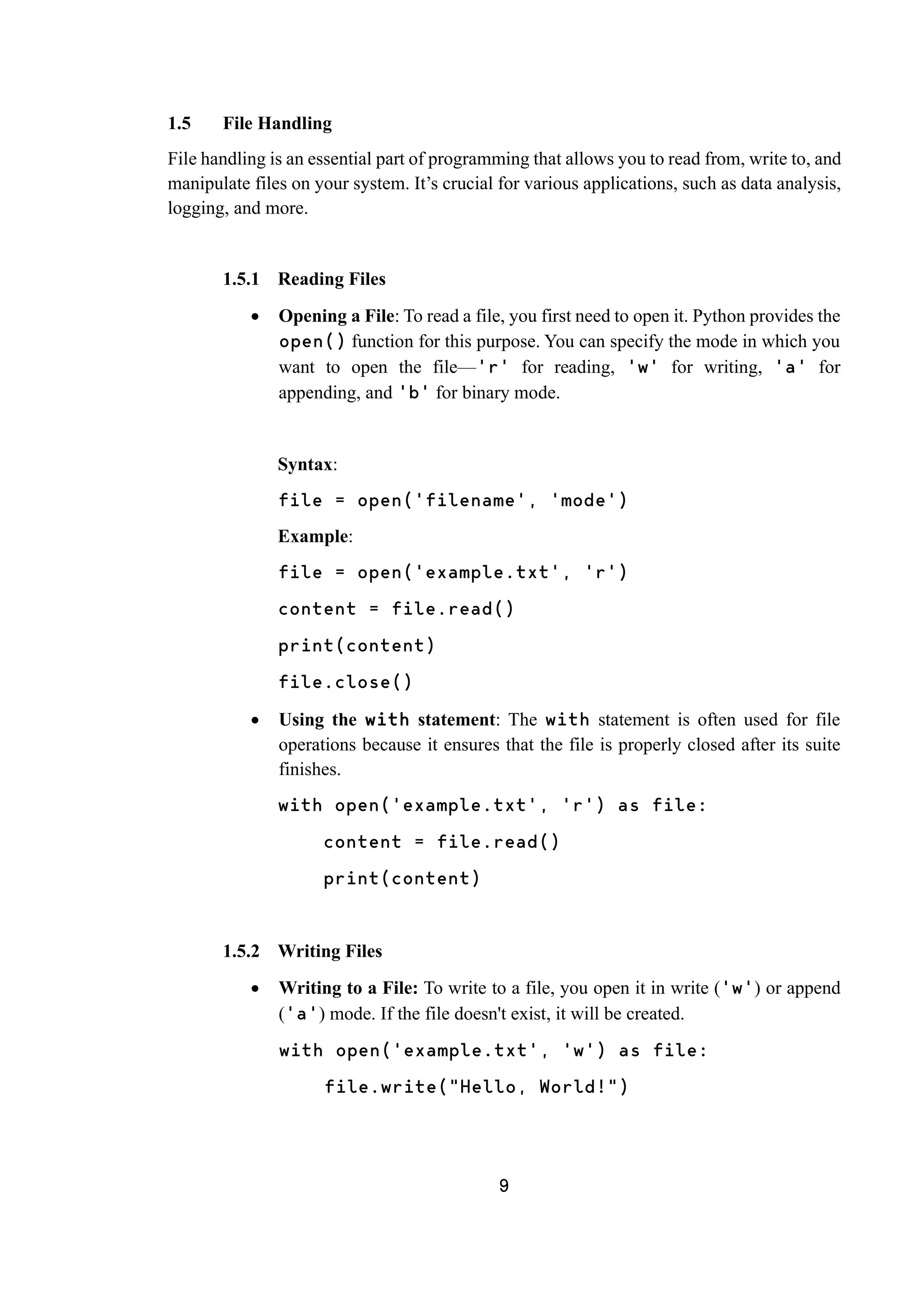
10  Appending to a File: Appending adds new content to the end of the file without overwriting existing content. with open('example.txt', 'a') as file: file.write("nThis is an appended line.") 1.5.3 Working with CSV Files CSV (Comma-Separated Values) files are commonly used for storing tabular data. Python provides the csv module to work with CSV files.  Reading CSV Files: import csv with open('data.csv', 'r') as file: reader = csv.reader(file) for row in reader: print(row)  Writing to CSV Files: import csv with open('data.csv', 'w', newline='') as file: writer = csv.writer(file) writer.writerow(['Name', 'Age', 'City']) writer.writerow(['Alice', 25, 'New York']) writer.writerow(['Bob', 30, 'San Francisco'])  Reading CSV Files into a Dictionary: Sometimes, it’s more convenient to read CSV data into a dictionary. import csv with open('data.csv', 'r') as file: reader = csv.DictReader(file)

11 for row in reader: print(dict(row))  Writing to CSV Files from a Dictionary: import csv data = [ {'Name': 'Alice', 'Age': 25, 'City': 'New York'}, {'Name': 'Bob', 'Age': 30, 'City': 'San Francisco'} ] with open('data.csv', 'w', newline='') as file: fieldnames = ['Name', 'Age', 'City'] writer = csv.DictWriter(file, fieldnames=fieldnames) writer.writeheader() for row in data: writer.writerow(row)

12 Chapter – 2 PYTHON DATAARRANGEMENT FORMATS 2.1 Lists and Tuples Lists and tuples in Python are both used to store collections of items, but they serve slightly different purposes due to their inherent properties. Lists, which are enclosed in square brackets, are mutable, meaning that the contents can be changed after they are created. This flexibility allows for modifications such as adding, removing, or altering elements within the list. This makes lists particularly useful for scenarios where the data set needs to be dynamic or updated frequently. For example, lists are often used to store sequences of data that will change, such as user inputs, configurations that may need to be adjusted, or data that evolves over the course of a program's execution. The ability to change the list makes it versatile for a wide range of applications, from simple data aggregation to complex data manipulation tasks in various domains, including web development, data analysis, and machine learning. On the other hand, tuples are enclosed in parentheses and are immutable, meaning once they are created, their contents cannot be altered. This immutability provides a form of integrity and security, ensuring that the data cannot be changed accidentally or intentionally, which can be crucial for maintaining consistent data states. Tuples are often used to represent fixed collections of items, such as coordinates, RGB colour values, or any data set that should remain constant throughout the program. The immutability of tuples can lead to more predictable and bug-free code, as developers can be certain that the data will not be altered. Additionally, because they are immutable, tuples can be used as keys in dictionaries, which require immutable types. This makes tuples suitable for scenarios where constant and unchanging data is necessary, enhancing both the readability and reliability of the code. 2.1.1 Creating Lists and Tuples  Creating a List: A list is created by placing all the items (elements) inside square brackets [], separated by commas. my_list = [1, 2, 3, 4, 5]  Creating a Tuple: A tuple is created by placing all the items (elements) inside parentheses (), separated by commas. my_tuple = (1, 2, 3, 4, 5)

13 2.1.2 Basic Operations Both lists and tuples support common operations such as indexing, slicing, and iteration.  Indexing: You can access individual elements using an index. Indexing starts from 0. print(my_list[0]) # Outputs: 1 print(my_tuple[1]) # Outputs: 2  Slicing: You can access a range of elements using slicing. print(my_list[1:3]) # Outputs: [2, 3] print(my_tuple[:4]) # Outputs: (1, 2, 3, 4)  Iteration: You can loop through the elements using a for loop. for item in my_list: print(item) for item in my_tuple: print(item) 2.1.3 List and Tuple Methods Lists have several built-in methods that allow modification. Tuples, being immutable, have fewer methods.  List Methods:  append(): Adds an item to the end of the list. my_list.append(6) print(my_list) # Outputs: [1, 2, 3, 4, 5, 6]  remove(): Removes the first occurrence of an item. my_list.remove(3) print(my_list) # Outputs: [1, 2, 4, 5, 6]  insert(): Inserts an item at a specified position. my_list.insert(2, 'a') print(my_list) # Outputs: [1, 2, 'a', 4, 5, 6]

14  pop(): Removes and returns the item at a given position. If no index is specified, removes and returns the last item. my_list.pop() print(my_list) # Outputs: [1, 2, 'a', 4, 5]  Tuple Methods:  count(): Returns the number of times a specified value occurs in a tuple. print(my_tuple.count(2)) # Outputs: 1  index(): Searches the tuple for a specified value and returns the position of where it was found. print(my_tuple.index(3)) # Outputs: 2 2.2 Dictionaries and Sets Dictionaries and sets are fundamental data structures in Python, each with distinct characteristics that make them suitable for different scenarios, especially in object-oriented programming and machine learning contexts. Dictionaries, often called associative arrays or hash maps in other programming languages, store data as key-value pairs, allowing for efficient data retrieval based on unique keys. This makes dictionaries particularly useful for tasks where quick lookup, insertion, and deletion of data are critical. For instance, dictionaries are invaluable in machine learning for managing datasets, where feature names (keys) are mapped to their values, or for storing model parameters and configurations. Their ability to handle complex data associations dynamically makes them a versatile tool in both data preprocessing and algorithm implementation. Sets, on the other hand, are collections of unique elements, which makes them ideal for operations involving membership tests, duplicates removal, and mathematical operations like unions, intersections, and differences. In the context of machine learning, sets are often used to handle unique elements such as in feature selection processes, where ensuring that each feature is considered only once is crucial.Additionally, sets are employed to efficiently manage and analyze datasets by quickly identifying and eliminating duplicates, thus maintaining data integrity. Both dictionaries and sets contribute significantly to the robustness and efficiency of programming solutions, providing the tools needed to handle various data-centric tasks with precision and ease. Their distinct properties—dictionaries with their key-value mappings and sets with their uniqueness constraints—complement each other and enhance the flexibility and performance of Python applications in both everyday programming and specialized fields like machine learning.

15 2.2.1 Creating Dictionaries and Sets  Dictionaries: Dictionaries are collections of key-value pairs. Each key maps to a specific value, and keys must be unique. Dictionaries are created using curly braces {} with a colon separating keys and values. my_dict = {'name': 'Alice', 'age': 25, 'city': 'New York'}  Sets: Sets are unordered collections of unique elements. Sets are created using curly braces {} or the set() function. my_set = {1, 2, 3, 4, 5} 2.2.2 Basic Operations  Dictionaries:  Accessing Values: You can access dictionary values using their keys. print(my_dict['name']) # Outputs: Alice  Adding/Updating Elements: You can add new key-value pairs or update existing ones. my_dict['age'] = 26 # Updates age to 26  Removing Elements: You can remove elements using the del statement or pop() method. del my_dict['city'] # Removes the key 'city'  Sets:  Adding Elements: Use the add() method to add elements to a set. my_set.add(6) # Adds 6 to the set  Removing Elements: Use the remove() or discard() method to remove elements. my_set.remove(3) # Removes 3 from the set  Set Operations: Sets support mathematical operations like union, intersection, and difference. another_set = {4, 5, 6, 7} union_set = my_set.union(another_set) # {1, 2, 4, 5, 6, 7}

16 2.2.3 Dictionary and Set Methods  Dictionary Methods:  keys(): Returns a view object that displays a list of all the keys in the dictionary. print(my_dict.keys()) # Outputs: dict_keys(['name', 'age'])  values(): Returns a view object that displays a list of all the values in the dictionary. print(my_dict.values()) # Outputs: dict_values(['Alice', 26])  items(): Returns a view object that displays a list of dictionary's key- value tuple pairs. print(my_dict.items()) # Outputs: dict_items([('name', 'Alice'), ('age', 26)])  Set Methods:  union(): Returns a new set containing all elements from both sets. union_set = my_set.union(another_set) # {1, 2, 4, 5, 6, 7}  intersection(): Returns a new set containing only elements that are common to both sets. intersection_set = my_set.intersection (another_set) # {4, 5}  difference(): Returns a new set containing elements that are in the first set but not in the second. difference_set = my_set.difference(another_set) # {1, 2} 2.3 Arrays Arrays are one of the most fundamental data structures in computer science. They provide a way to store a fixed-size sequential collection of elements of the same type. Arrays are widely used because they offer efficient access to elements by their index and support various operations that are foundational for many algorithms.

17 2.3.1 Creating Arrays in Python The closest native data structure to arrays is the list, but for more efficiency with numerical operations, the array module or NumPy arrays are often used.  Using the array Module: import array # Creating an array of integers arr = array.array('i', [1, 2, 3, 4, 5]) print(arr) # Outputs: array('i', [1, 2, 3, 4, 5]) # Accessing elements by index print(arr[0]) # Outputs: 1 # Modifying elements arr[1] = 10 print(arr) # Outputs: array('i', [1, 10, 3, 4, 5])  Using NumPy Arrays: import numpy as np # Creating a NumPy array arr = np.array([1, 2, 3, 4, 5]) print(arr) # Outputs: [1 2 3 4 5] # Accessing elements by index print(arr[0]) # Outputs: 1 # Modifying elements arr[1] = 10 print(arr) # Outputs: [ 1 10 3 4 5]

18 # Performing operations on arrays print(arr + 2) # Outputs: [ 3 12 5 6 7] print(arr * 2) # Outputs: [ 2 20 6 8 10] 2.3.2 Applications of Arrays in Algorithms  Sorting Algorithms: Arrays are often used in sorting algorithms such as Quick Sort, Merge Sort, and Bubble Sort. Sorting algorithms typically operate on arrays due to their efficient access and modification capabilities.  Searching Algorithms: Arrays are used in searching algorithms such as Linear Search and Binary Search. Arrays provide a straightforward way to store data sequentially, making it easier to search through them.  Dynamic Programming: Arrays are crucial in dynamic programming to store intermediate results and avoid redundant calculations. This helps in optimizing the time complexity of algorithms.

19 Chapter – 3 DATA STRUCTURE 3.1 Introduction Data structures are specialized formats for organizing, processing, and storing data. 3.1.1 Primitive Data Structures: These are basic structures that hold single values. They are the simplest form of data storage.  Integers  Floats  Characters  Booleans 3.1.2 Non-Primitive Data Structures: These are more complex structures that can hold multiple values and can be used to store collections of data.  Linear: These data structures store data in a linear or sequential order. Every element has a single predecessor and a single successor (except the first and last elements).  Arrays  Linked List  Stacks  Queues  Non-Linear Data Structures: These data structures store data in a hierarchical manner and do not necessarily follow a sequential order. Each element can be connected to multiple elements, reflecting complex relationships.  Trees  Graphs

20 3.2 Linked List A linked list is a linear data structure where elements are stored in nodes. Each node contains two parts: data and a reference (or link) to the next node in the sequence.  Singly Linked List  Doubly Linked List  Circular Linked List 3.2.1 Singly Linked List Each node in a singly linked list points to the next node. The last node points to null, indicating the end of the list. class Node: def __init__(self, data): self.data = data self.next = None class SinglyLinkedList: def __init__(self): self.head = None 3.2.2 Doubly Linked List Each node has two references: one to the next node and another to the previous node. This allows traversal in both directions. class Node: def __init__(self, data): self.data = data self.next = None self.prev = None class DoublyLinkedList: def __init__(self): self.head = None

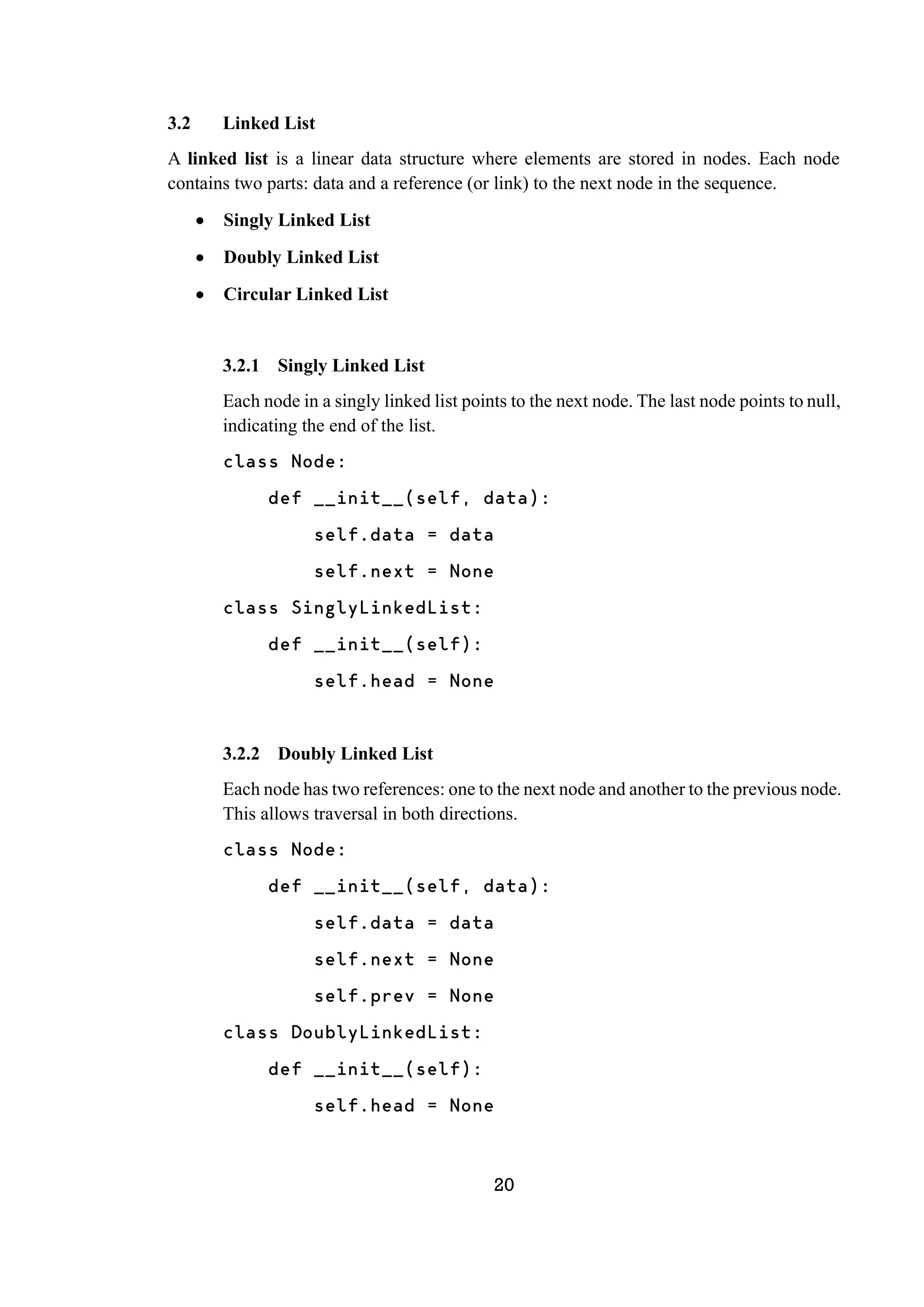
21 3.2.3 Circular Linked List In a circular linked list, the last node points back to the first node, forming a circle. It can be singly or doubly linked. (Using Singly Circular) class Node: def __init__(self, data): self.data = data self.next = None class CircularLinkedList: def __init__(self): self.head = None 3.2.4 Memory Usage  Singly Linked List: Requires memory for the data and a pointer to the next node.  Doubly Linked List: Requires memory for the data, a pointer to the next node, and a pointer to the previous node.  Circular Linked List: Similar to singly or doubly linked lists in memory usage, but with the last node pointing back to the first node. 3.3 Stack A stack is a linear data structure that follows a particular order for operations. The order may be LIFO (Last In First Out) or FILO (First In Last Out). class Stack: def __init__(self): self.items = [] def push(self, item): self.items.append(item) def pop(self): if not self.is_empty():

22 return self.items.pop() def peek(self): if not self.is_empty(): return self.items[-1] def is_empty(self): return len(self.items) == 0 def size(self): return len(self.items) # Example usage stack = Stack() stack.push(1) stack.push(2) stack.push(3) print(stack.peek()) # Output: 3 print(stack.pop()) # Output: 3 print(stack.pop()) # Output: 2 print(stack.size()) # Output: 1 3.3.1 LIFO Principle The LIFO (Last In, First Out) principle means that the last element added to the stack will be the first one to be removed. Think of it like a stack of plates: the last plate placed on top is the first one to be taken off. 3.3.2 Common Operations  Push:  Adds an element to the top of the stack.  Time Complexity: O(1) (since adding an element to the end of the list is a constant-time operation).

23  Pop:  Removes and returns the top element of the stack.  Time Complexity: O(1) (since removing an element from the end of the list is a constant-time operation).  Peek:  Returns the top element of the stack without removing it.  Time Complexity: O(1) (since accessing the last element of the list is a constant-time operation). 3.3.3 Memory Usage Memory usage for a stack is generally O(n), where n is the number of elements in the stack. This is because we need to store each element in memory. 3.4 Queue A queue is a linear data structure that follows the First In, First Out (FIFO) principle. This means that the first element added to the queue will be the first one to be removed.  Simple Queue  Circular Queue  Priority Queue 3.4.1 FIFO Principle The FIFO (First In, First Out) principle is analogous to a line of people at a ticket counter. The first person to join the line is the first one to be served and leave the line. 3.4.2 Simple Queue A simple queue operates on the FIFO principle. Elements are added at the rear and removed from the front. class SimpleQueue: def __init__(self): self.queue = []

24 def enqueue(self, item): self.queue.append(item) def dequeue(self): if not self.is_empty(): return self.queue.pop(0) def is_empty(self): return len(self.queue) == 0 def front(self): if not self.is_empty(): return self.queue[0] # Example usage queue = SimpleQueue() queue.enqueue(1) queue.enqueue(2) queue.enqueue(3) print(queue.front()) # Output: 1 print(queue.dequeue()) # Output: 1 print(queue.dequeue()) # Output: 2 print(queue.is_empty()) # Output: False 3.4.3 Circular Queue In a circular queue, the last position is connected back to the first position to form a circle. This improves the utilization of space. class CircularQueue: def __init__(self, size): self.queue = [None] * size self.max_size = size self.front = -1

25 self.rear = -1 def enqueue(self, item): if ((self.rear + 1) % self.max_size == self.front): print("Queue is full") elif self.front == -1: self.front = 0 self.rear = 0 self.queue[self.rear] = item else: self.rear = (self.rear + 1) % self.max_size self.queue[self.rear] = item def dequeue(self): if self.front == -1: print("Queue is empty") elif self.front == self.rear: temp = self.queue[self.front] self.front = -1 self.rear = -1 return temp else: temp = self.queue[self.front] self.front = (self.front + 1) % self.max_size return temp def is_empty(self): return self.front == -1 def front(self): if self.is_empty(): return None

26 return self.queue[self.front] # Example usage circular_queue = CircularQueue(5) circular_queue.enqueue(1) circular_queue.enqueue(2) circular_queue.enqueue(3) print(circular_queue.front()) # Output: 1 print(circular_queue.dequeue()) # Output: 1 print(circular_queue.dequeue()) # Output: 2 print(circular_queue.is_empty()) # Output: False 3.4.4 Priority Queue In a priority queue, elements are removed based on their priority, not just their position in the queue. Higher priority elements are dequeued before lower priority elements. import heapq class PriorityQueue: def __init__(self): self.queue = [] def enqueue(self, item, priority): heapq.heappush(self.queue, (priority, item)) def dequeue(self): if not self.is_empty(): return heapq.heappop(self.queue)[1] def is_empty(self): return len(self.queue) == 0 def front(self):

27 if not self.is_empty(): return self.queue[0][1] # Example usage priority_queue = PriorityQueue() priority_queue.enqueue('A', 2) priority_queue.enqueue('B', 1) priority_queue.enqueue('C', 3) print(priority_queue.front()) # Output: B print(priority_queue.dequeue()) # Output: B print(priority_queue.dequeue()) # Output: A print(priority_queue.is_empty()) # Output: False 3.5 Hash A hash table is a data structure that maps keys to values. It uses a hash function to compute an index into an array of buckets or slots, from which the desired value can be found. Hash tables are highly efficient for lookups, insertions, and deletions. def simple_hash(key, size): return hash(key) % size size = 10 index = simple_hash("example", size) print(index) # This will print the index for the key "example" 3.5.1 Hashing Mechanisms Hashing is the process of converting a given key into a unique index. The hash function processes the input and returns a fixed-size string or number that typically serves as an index in the array.

28 3.5.2 Collision Resolution Techniques Since multiple keys can hash to the same index (a situation known as a collision), we need ways to handle these collisions. The two primary techniques are chaining and open addressing.  Chaining: In chaining, each bucket contains a linked list (or another secondary data structure) of all elements that hash to the same index. This way, multiple values can be stored at each index.  Open Addressing: In open addressing, when a collision occurs, the algorithm searches for the next available slot within the table itself. There are several strategies for open addressing, including linear probing, quadratic probing, and double hashing. 3.6 Tree A tree is a non-linear hierarchical data structure that consists of nodes connected by edges. Each node contains a value, and nodes are organized in a hierarchical manner. The topmost node is called the root, and each node has zero or more child nodes.  Binary Tree  Binary Search Tree (BST) 3.6.1 Binary Tree A binary tree is a type of tree where each node has at most two children, referred to as the left child and the right child. class Node: def __init__(self, data): self.data = data self.left = None self.right = None class BinaryTree: def __init__(self): self.root = None

29 3.6.2 Binary Search Tree (BST) Abinary search tree (BST) is a binary tree with the additional property that for any given node, the value of the left child is less than the value of the node, and the value of the right child is greater than the value of the node. This property makes searching operations efficient. class Node: def __init__(self, data): self.data = data self.left = None self.right = None class BinarySearchTree: def __init__(self): self.root = None def insert(self, data): if self.root is None: self.root = Node(data) else: self._insert(self.root, data) def _insert(self, current_node, data): if data < current_node.data: if current_node.left is None: current_node.left = Node(data) else: self._insert(current_node.left, data) elif data > current_node.data: if current_node.right is None: current_node.right = Node(data) else: self._insert(current_node.right, data)

30 3.6.3 Traversal Method Tree traversal methods are used to visit all the nodes in a tree and perform an operation (e.g., printing the node's value) on each node. The three common traversal methods for binary trees are in-order, pre-order, and post-order.  In-order Traversal:  Traverse the left subtree  Visit the root node  Traverse the right subtree  Pre-order Traversal:  Visit the root node  Traverse the left subtree  Traverse the right subtree  Post-order Traversal:  Traverse the left subtree  Traverse the right subtree  Visit the root node 3.7 Graph A graph is a data structure that consists of a finite set of vertices (or nodes) and a set of edges connecting them. Graphs are used to model pairwise relations between objects.  Directed Graph  Undirected Graph 3.8.1 Directed Graph (Digraph) In a directed graph, edges have a direction. This means that each edge is an ordered pair of vertices, representing a one-way relationship. A → B → C In this example, you can go from A to B and from B to C, but not the other way around.

31 3.7.2 Undirected Graph In an undirected graph, edges do not have a direction. Each edge is an unordered pair of vertices, representing a two-way relationship. A - B – C In this example, you can travel between A and B or B and C in either direction. 3.8.3 Representation Graphs can be represented in several ways, with the most common being the adjacency matrix and adjacency list.  Adjancency Matrix: An adjacency matrix is a 2D array of size V x V where V is the number of vertices. If there is an edge from vertex i to vertex j, then the matrix at position (i, j) will be 1 (or the weight of the edge if it's weighted). Otherwise, it will be 0.  Adjacency List:An adjacency list is an array of lists. The array size is equal to the number of vertices. Each entry i in the array contains a list of vertices to which vertex i is connected. 3.8 Heap A heap is a specialized tree-based data structure that satisfies the heap property. In a heap, for every node i, the value of i is either greater than or equal to (in a max-heap) or less than or equal to (in a min-heap) the value of its children, if they exist. 3.9.1 Min-Heap vs Max-Heap  Min-Heap: In a min-heap, the value of the parent node is always less than or equal to the values of its children. The root node has the smallest value. 1 / 3 2 / 4 5

32  Max-Heap: In a max-heap, the value of the parent node is always greater than or equal to the values of its children. The root node has the largest value 5 / 3 4 / 1 2 3.8.2 Common Operations  Insert: Inserting an element into a heap involves adding the new element to the end of the heap and then restoring the heap property by comparing the new element with its parent and swapping if necessary. This process is called "heapifying up". class MinHeap: def __init__(self): self.heap = [] def insert(self, key): self.heap.append(key) self._heapify_up(len(self.heap) - 1) def _heapify_up(self, index): parent_index = (index - 1) // 2 if index > 0 and self.heap[index] < self.heap[parent_index]: self.heap[index], self.heap[parent_index] = self.heap[parent_index], self.heap[index] self._heapify_up(parent_index) # Example usage min_heap = MinHeap() min_heap.insert(3)

33 min_heap.insert(1) min_heap.insert(6) min_heap.insert(5) print(min_heap.heap) # Output: [1, 3, 6, 5]  Delete (Extract Min/Max): Deleting the root element from a heap involves removing the root and replacing it with the last element in the heap. The heap property is then restored by comparing the new root with its children and swapping if necessary. This process is called "heapifying down". (Max-Heap) def delete_min(self): if len(self.heap) == 0: return None if len(self.heap) == 1: return self.heap.pop() root = self.heap[0] self.heap[0] = self.heap.pop() self._heapify_down(0) return root def _heapify_down(self, index): smallest = index left_child = 2 * index + 1 right_child = 2 * index + 2 if left_child < len(self.heap) and self.heap[left_child] < self.heap[smallest]: smallest = left_child if right_child < len(self.heap) and self.heap[right_child] < self.heap[smallest]: smallest = right_child if smallest != index:

34 self.heap[index], self.heap[smallest] = self.heap[smallest], self.heap[index] self._heapify_down(smallest)  Peek: Peeking at the heap returns the root element without removing it. In a min-heap, this is the smallest element; in a max-heap, this is the largest element. def peek(self): if len(self.heap) > 0: return self.heap[0] return None

35 Chapter – 4 ALGORITHMS 4.1 Introduction An algorithm is a step-by-step procedure or formula for solving a problem. They are essential building blocks in computer science and are used to automate tasks and solve complex problems efficiently.  Search Algorithms  Divide and Conquer  Sorting Algorithms  Greedy Algorithms  Backtracking  Graph Algorithms  Bit Manipulation 4.2 Time and Space Complexity Time and space complexity are metrics used to analyze the efficiency of an algorithm. They help us understand how the algorithm performs as the input size grows.  Time Complexity: This measures the amount of time an algorithm takes to complete as a function of the size of the input. It's usually expressed using Big O notation (e.g., O(n), O(log n)), which gives an upper bound on the growth rate.  Space Complexity: This measures the amount of memory an algorithm uses in relation to the size of the input. Like time complexity, it's also expressed using Big O notation. 4.2.1 Why is it Necessary? Understanding time and space complexity is crucial for several reasons:  Efficiency: Helps in choosing the most efficient algorithm for a given problem.  Scalability: Ensures that the algorithm can handle large inputs.

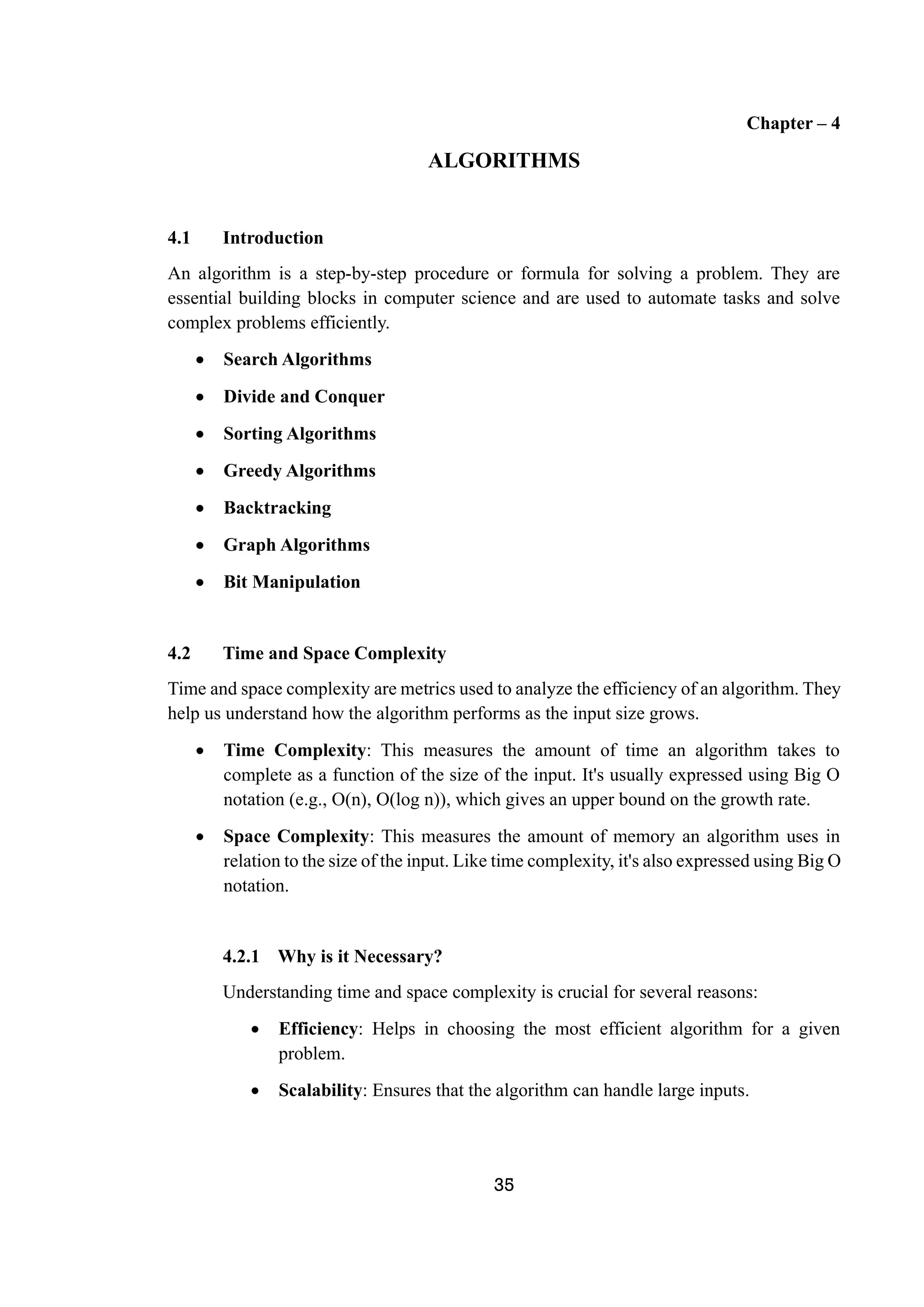
36  Optimization: Helps in identifying potential bottlenecks and optimizing the code.  Resource Management: Ensures efficient use of computational resources. 4.2.3 How to Calculate Time and Space Complexity? Let's consider an example in Python to illustrate this. Calculating the Sum of a List: def sum_of_list(nums): total = 0 # O(1) space for num in nums: # Loop runs 'n' times, where 'n' is the length of the list total += num # O(1) space for the addition return total # O(1) time # Example usage numbers = [1, 2, 3, 4, 5] result = sum_of_list(numbers) print(result) Time Complexity Analysis:  Initialization: total = 0 takes constant time, O(1).  Loop: The loop runs 'n' times, where 'n' is the length of the list, so this is O(n).  Addition: Adding each element takes constant time, O(1). Overall, the time complexity is O(n). Space Complexity Analysis:  Variables: total uses O(1) space.  Input list: The input list nums itself takes O(n) space. Overall, the space complexity is O(n).

37 4.3 Search Algorithms Used to search for an element within a data structure.  Linear Search  Binary Search  Depth-First Search (DFS)  Breadth-First Search (BFS) 4.3.1 Linear Search Linear search is the simplest search algorithm. It checks every element in the list sequentially until the target value is found or the list ends. def linear_search(arr, target): for i in range(len(arr)): if arr[i] == target: return i # Return the index of the target return -1 # Return -1 if the target is not found # Example usage arr = [3, 5, 1, 4, 2] target = 4 print(linear_search(arr, target)) # Output: 3 4.3.2 Binary Search Binary search is an efficient algorithm for finding an item from a sorted list of items. It works by repeatedly dividing the search interval in half. def binary_search(arr, target): left, right = 0, len(arr) - 1 while left <= right: mid = (left + right) // 2 if arr[mid] == target: return mid # Return the index of the target

38 elif arr[mid] < target: left = mid + 1 else: right = mid - 1 return -1 # Return -1 if the target is not found # Example usage arr = [1, 2, 3, 4, 5] target = 3 print(binary_search(arr, target)) # Output: 2 4.3.3 Depth-First Search (DFS) Depth-first search (DFS) is a graph traversal algorithm that starts at the root node and explores as far as possible along each branch before backtracking. def dfs(graph, start, visited=None): if visited is None: visited = set() visited.add(start) print(start, end=' ') for neighbor in graph[start]: if neighbor not in visited: dfs(graph, neighbor, visited) # Example usage graph = { 'A': ['B', 'C'], 'B': ['D', 'E'], 'C': ['F'],

39 'D': [], 'E': ['F'], 'F': [] } dfs(graph, 'A') # Output: A B D E F C 4.3.4 Breadth-First Search (BFS) Breadth-first search (BFS) is a graph traversal algorithm that starts at the root node and explores all neighbors at the present depth before moving on to nodes at the next depth level. from collections import deque def bfs(graph, start): visited = set() queue = deque([start]) visited.add(start) while queue: vertex = queue.popleft() print(vertex, end=' ') for neighbor in graph[vertex]: if neighbor not in visited: visited.add(neighbor) queue.append(neighbor) # Example usage graph = { 'A': ['B', 'C'], 'B': ['D', 'E'], 'C': ['F'], 'D': [],

40 'E': ['F'], 'F': [] } bfs(graph, 'A') # Output: A B C D E F 4.4 Divide and Conquer Divide and Conquer is an algorithmic paradigm that involves breaking a problem into smaller subproblems, solving each subproblem independently, and then combining their solutions to solve the original problem. This approach is particularly effective for problems that can be recursively divided into similar subproblems.  Merge Sort  Quick Sort  Binary Search 4.4.1 Steps in Divide and Conquer  Divide: Break the problem into smaller subproblems of the same type.  Conquer: Solve the subproblems recursively.  Combine: Merge the solutions of the subproblems to get the solution to the original problem. 4.5 Sorting Algorithms Used to arrange data in a particular order.  Bubble Sort  Merge Sort  Quick Sort 4.5.1 Bubble Sort Bubble Sort is a simple comparison-based sorting algorithm. It works by repeatedly stepping through the list, comparing adjacent elements, and swapping them if they are in the wrong order. This process is repeated until the list is sorted.

41 def bubble_sort(arr): n = len(arr) for i in range(n): for j in range(0, n-i-1): if arr[j] > arr[j+1]: arr[j], arr[j+1] = arr[j+1], arr[j] return arr # Example usage arr = [64, 34, 25, 12, 22, 11, 90] print(bubble_sort(arr)) # Output: [11, 12, 22, 25, 34, 64, 90] Time Complexity:  Worst and Average Case: O(n2 )  Best Case: O(n) (when the array is already sorted) 4.5.2 Merge Sort Merge Sort is a divide and conquer algorithm. It divides the input array into two halves, calls itself for the two halves, and then merges the two sorted halves. def merge_sort(arr): if len(arr) > 1: mid = len(arr) // 2 left_half = arr[:mid] right_half = arr[mid:] merge_sort(left_half) merge_sort(right_half) i = j = k = 0 while i < len(left_half) and j < len(right_half): if left_half[i] < right_half[j]:

42 arr[k] = left_half[i] i += 1 else: arr[k] = right_half[j] j += 1 k += 1 while i < len(left_half): arr[k] = left_half[i] i += 1 k += 1 while j < len(right_half): arr[k] = right_half[j] j += 1 k += 1 return arr # Example usage arr = [38, 27, 43, 3, 9, 82, 10] print(merge_sort(arr)) # Output: [3, 9, 10, 27, 38, 43, 82] Time Complexity:  Worst, Average, and Best Case: O(n log n) 4.5.3 Quick Sort Quick Sort is a divide and conquer algorithm. It selects a 'pivot' element and partitions the array around the pivot, such that elements on the left of the pivot are less than the pivot and elements on the right are greater. The process is then recursively applied to the sub-arrays. This leads to an efficient sorting process with an average time complexity of O(n log n). Additionally, Quick Sort is often faster in practice due to its efficient cache performance and reduced overhead from fewer memory writes compared to other sorting algorithms like Merge Sort.

43 def partition(arr, low, high): pivot = arr[high] i = low - 1 for j in range(low, high): if arr[j] <= pivot: i += 1 arr[i], arr[j] = arr[j], arr[i] arr[i + 1], arr[high] = arr[high], arr[i + 1] return i + 1 def quick_sort(arr, low, high): if low < high: pi = partition(arr, low, high) quick_sort(arr, low, pi - 1) quick_sort(arr, pi + 1, high) return arr # Example usage arr = [10, 7, 8, 9, 1, 5] print(quick_sort(arr, 0, len(arr) - 1)) # Output: [1, 5, 7, 8, 9, 10] Time Complexity:  Worst Case: O(n2 ) (when the pivot is the smallest or largest element)  Average and Best Case: O(n log n) 4.6 Greedy Algorithms Greedy algorithms are a type of algorithmic paradigm that makes a series of choices by selecting the best option available at each step. The goal is to find an overall optimal solution by making a locally optimal choice at each stage.

44 4.6.1 Prim’s Algorithm Prim's algorithm is a greedy algorithm that finds the Minimum Spanning Tree (MST) for a weighted undirected graph. The MST is a subset of the edges that connects all vertices in the graph with the minimum total edge weight and without any cycles. import heapq def prims_algorithm(graph, start): mst = [] visited = set() min_heap = [(0, start)] # (weight, vertex) while min_heap: weight, current_vertex = heapq.heappop(min_heap) if current_vertex in visited: continue visited.add(current_vertex) mst.append((weight, current_vertex)) for neighbor, edge_weight in graph[current_vertex]: if neighbor not in visited: heapq.heappush(min_heap, (edge_weight, neighbor)) return mst # Example usage graph = { 'A': [('B', 1), ('C', 3)], 'B': [('A', 1), ('C', 7), ('D', 5)], 'C': [('A', 3), ('B', 7), ('D', 12)], 'D': [('B', 5), ('C', 12)]

45 } mst = prims_algorithm(graph, 'A') print(mst) # Output: [(0, 'A'), (1, 'B'), (5, 'D'), (3, 'C')] Steps of Prim’s Algorithm:  Initialize a tree with a single vertex, chosen arbitrarily from the graph.  Grow the tree by one edge: choose the minimum weight edge from the graph that connects a vertex in the tree to a vertex outside the tree.  Repeat step 2 until all vertices are included in the tree. 4.7 Backtracking Backtracking is an algorithmic paradigm that tries to build a solution incrementally, one piece at a time. It removes solutions that fail to meet the conditions of the problem at any point in time (called constraints) as soon as it finds them. Backtracking is useful for solving constraint satisfaction problems, where you need to find an arrangement or combination that meets specific criteria.  N-Queen’s Algorithm 4.7.1 N-Queen’s Algorithm The N-Queens problem involves placing N queens on an N×N chessboard so that no two queens threaten each other. This means no two queens can share the same row, column, or diagonal. This classic problem is a perfect example of a backtracking algorithm. Solutions are found by placing queens one by one in different columns, starting from the leftmost column, and backtracking when a conflict is detected. def is_safe(board, row, col, N): for i in range(col): if board[row][i] == 1: return False for i, j in zip(range(row, -1, -1), range(col, -1, -1)): if board[i][j] == 1:

46 return False for i, j in zip(range(row, N, 1), range(col, -1, -1)): if board[i][j] == 1: return False return True def solve_n_queens_util(board, col, N): if col >= N: return True for i in range(N): if is_safe(board, i, col, N): board[i][col] = 1 if solve_n_queens_util(board, col + 1, N): return True board[i][col] = 0 # Backtrack return False def solve_n_queens(N): board = [[0] * N for _ in range(N)] if not solve_n_queens_util(board, 0, N): return "Solution does not exist" return board # Example usage N = 4 solution = solve_n_queens(N) for row in solution: print(row)

47 Output: [0, 0, 1, 0] [1, 0, 0, 0] [0, 0, 0, 1] [0, 1, 0, 0] 4.8 Graph Algorithm Graph algorithms are used to solve problems related to graph theory, which involves vertices (or nodes) and edges connecting them. These algorithms help in understanding and manipulating the structure and properties of graphs. Here are some of the most important graph algorithms:  Dijkstra’s Algorithm 4.8.1 Dijkstra’s Algorithm Dijkstra's algorithm is used to find the shortest path from a source vertex to all other vertices in a graph with non-negative edge weights. It uses a priority queue to repeatedly select the vertex with the smallest distance, updates the distances of its neighbors, and continues until all vertices have been processed. import heapq def dijkstra(graph, start): distances = {vertex: float('infinity') for vertex in graph} distances[start] = 0 priority_queue = [(0, start)] while priority_queue: current_distance, current_vertex = heapq.heappop(priority_queue) if current_distance > distances[current_vertex]: continue for neighbor, weight in graph[current_vertex]:

48 distance = current_distance + weight if distance < distances[neighbor]: distances[neighbor] = distance heapq.heappush(priority_queue, (distance, neighbor)) return distances # Example usage graph = { 'A': [('B', 1), ('C', 4)], 'B': [('A', 1), ('C', 2), ('D', 5)], 'C': [('A', 4), ('B', 2), ('D', 1)], 'D': [('B', 5), ('C', 1)] } start_vertex = 'A' print(dijkstra(graph, start_vertex)) # Output: {'A': 0, 'B': 1, 'C': 3, 'D': 4} 4.8.2 Steps of Dijkstra’s Algorithm  Initialise: Set source vertex distance to 0; all other vertices to infinity. Add source vertex to the priority queue with distance 0.  Relaxation: Extract vertex with minimum distance. For each neighbor, update distances if a shorter path is found, and add neighbor to priority queue.  Repeat: Keep extracting the minimum distance vertex and updating neighbors until the priority queue is empty.

49 CONCLUSION In this enriching exploration of data structures and algorithms, a profound understanding has been unearthed, weaving a tapestry of computational elegance. The journey commenced with the foundations of linked lists, where the fluid interplay of singly, doubly, and circular variations showcased the graceful management of dynamic data. Through the orchestration of stacks and queues, the principles of LIFO and FIFO came to life, demonstrating the seamless handling of operations in a structured manner. Hash tables revealed the magic of hashing, where keys and values found their place through efficient collision resolution techniques. The branching paths of binary trees and the intricate networks of graphs, traversed through the methodologies of DFS and BFS, painted a vivid picture of hierarchical and interconnected data structures. As the narrative unfolded, the power of algorithms took center stage. Sorting algorithms like bubble, merge, and quick sort choreographed the transformation of unordered data into organized sequences, each with its distinct rhythm and efficiency. Greedy algorithms and backtracking illuminated the path to optimization and constraint satisfaction, with Prim's algorithm and the N-Queens problem exemplifying their prowess. The divide and conquer approach brought forth the beauty of breaking problems into manageable fragments, elegantly demonstrated by merge sort and binary search. The climax was marked by the elegance of Dijkstra's algorithm, a masterful technique that navigates the vertices of a graph to unveil the shortest paths with precision and clarity. This journey, rich with insights and computational artistry, stands as a testament to the profound depth and beauty of data structures and algorithms in the realm of computer science.

50 REFRENCES [1.] Carnes, B. (2021) Learn algorithms and data structures in Python. https://www.freecodecamp.org/news/learn-algorithms-and-data-structures-in- python/. [2.] DSA using Python (no date). https://premium.mysirg.com/learn/DSA-using- Python. [3.] GeeksforGeeks (2024) Learn DSA with Python | Python Data Structures and Algorithms. https://www.geeksforgeeks.org/python-data-structures-and- algorithms/. [4.] House of the Chronicles (no date). https://www.playbook.com/s/ayushbhattacharya/be4sABV1fU9xKKJ657f8okEr. [5.] Larson, Q. (2020) Python Data Science – a free 12-Hour course for beginners. Learn Pandas, NUMPy, Matplotlib, and more. https://www.freecodecamp.org/news/python-data-science-course-matplotlib- pandas-numpy/. [6.] Learn Data Structures and Algorithms with Python | Codecademy (no date). https://www.codecademy.com/learn/learn-data-structures-and-algorithms-with- python. [7.] Programming, data Structures and Algorithms using Python - course (no date). https://onlinecourses.nptel.ac.in/noc25_cs59/preview.

Data Structure and Algorithms (DSA) with Python

More Related Content

What's hot

Similar to Data Structure and Algorithms (DSA) with Python

Recently uploaded

Data Structure and Algorithms (DSA) with Python