Unit I Unit-1: INTRODUCTIONTO DATA SCIENCE 10 hours Benefits and uses of Data science, Facets of data, The data science process Introduction to Numpy: Numpy, creating array, attributes, Numpy Arrays objects: Creating Arrays, basic operations (Array Join, split, search, sort), Indexing, Slicing and iterating, copying arrays, Arrays shape manipulation, Identity array, eye function Exploring Data using Series, Exploring Data using Data Frames, Index objects, Re-index, Drop Entry, Selecting Entries, Data Alignment, Rank and Sort, Summary Statistics, Index Hierarchy Data Acquisition: Gather information from different sources, Web APIs, Open Data Sources, Web Scrapping.
3.
Big Data vsData Science • Big data is a blanket term for any collection of data sets so large or complex that it becomes difficult to process them using traditional data management techniques such as, for example, the RDBMS (relational database management systems). • Data science involves using methods to analyze massive amounts of data and extract the knowledge it contains. You can think of the relationship between big data and data science as being like the relationship between crude oil and an oil refinery.
4.
Characteristics of BigData • Volume—How much data is there? • Variety—How diverse are different types of data? • Velocity—At what speed is new data generated?
5.
Benefits and usesof data science and big data 1. It’s in Demand 2. Abundance of Positions 3. A Highly Paid Career 4. Data Science is Versatile 5. Data Science Makes Data Better 6. Data Scientists are Highly Prestigious 7. No More Boring Tasks 8. Data Science Makes Products Smarter 9. Data Science can Save Lives
6.
Facets of data ■Structured ■ Unstructured ■ Natural language ■ Machine-generated ■ Graph-based ■ Audio, video, and images ■ Streaming
7.
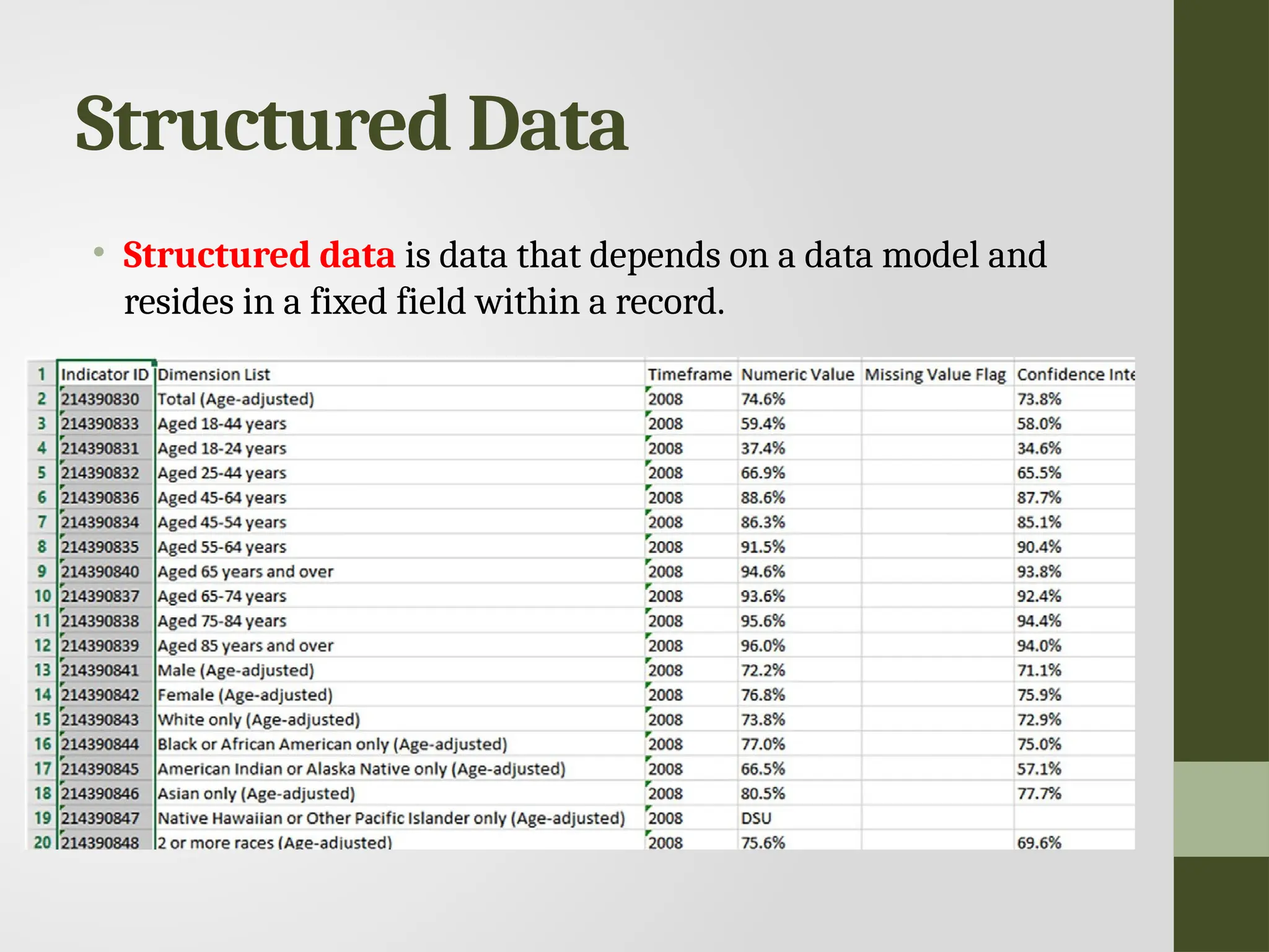
Structured Data • Structureddata is data that depends on a data model and resides in a fixed field within a record.
8.
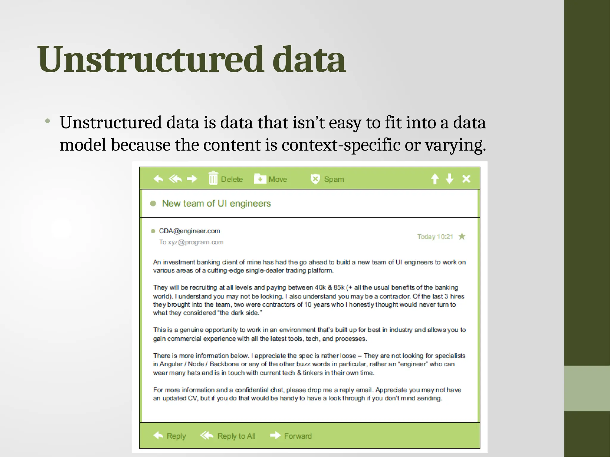
Unstructured data • Unstructureddata is data that isn’t easy to fit into a data model because the content is context-specific or varying.
9.
Natural language • Naturallanguage is a special type of unstructured data; it’s challenging to process because it requires knowledge of specific data science techniques and linguistics. • The natural language processing community has had success in entity recognition, topic recognition, summarization, text completion, and sentiment analysis, but models trained in one domain don’t generalize well to other domains.
10.
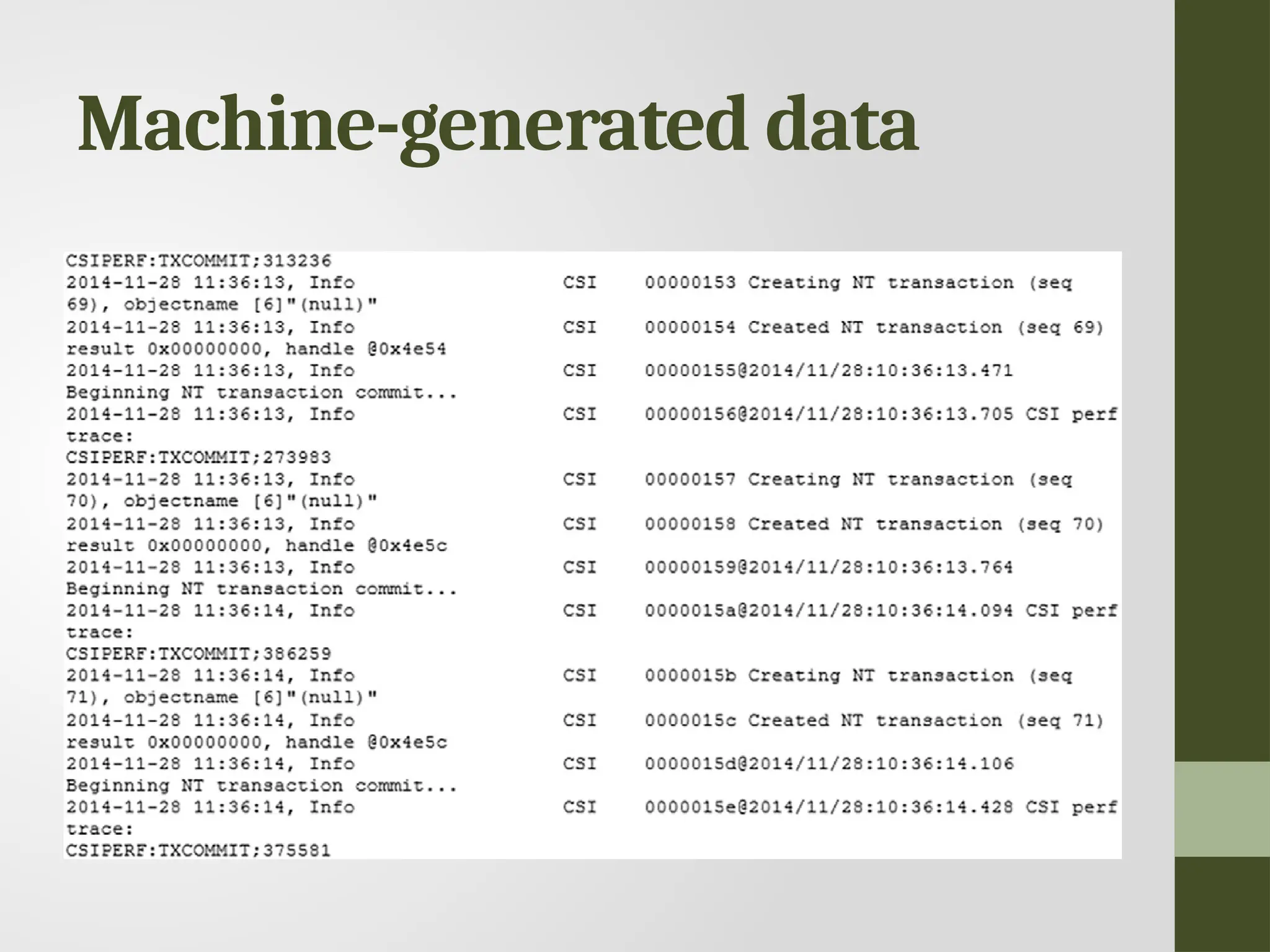
Machine-generated data • Machine-generateddata is information that’s automatically created by a computer, process, application, or other machine without human intervention. • Machine-generated data is becoming a major data resource and will continue to do so.
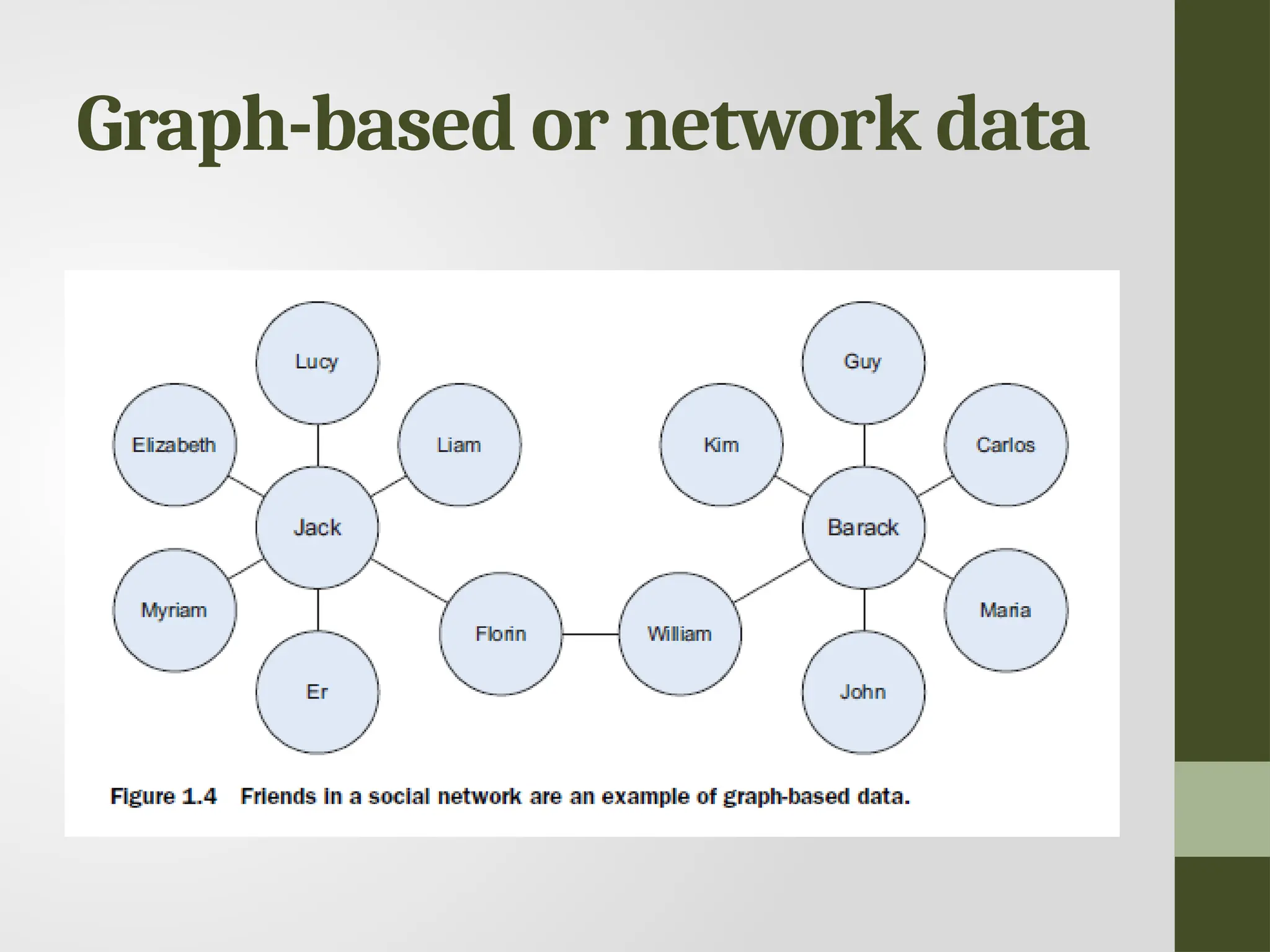
Graph-based or networkdata • “Graph data” can be a confusing term because any data can be shown in a graph. • “Graph” in this case points to mathematical graph theory. • In graph theory, a graph is a mathematical structure to model pair-wise relationships between objects. • Graph or network data is, in short, data that focuses on the relationship or adjacency of objects. • The graph structures use nodes, edges, and properties to represent and store graphical data. • Graph-based data is a natural way to represent social networks, and its structure allows you to calculate specific metrics such as the influence of a person and the shortest path between two people.
Audio, video andimage • Audio, image, and video are data types that pose specific challenges to a data scientist.
15.
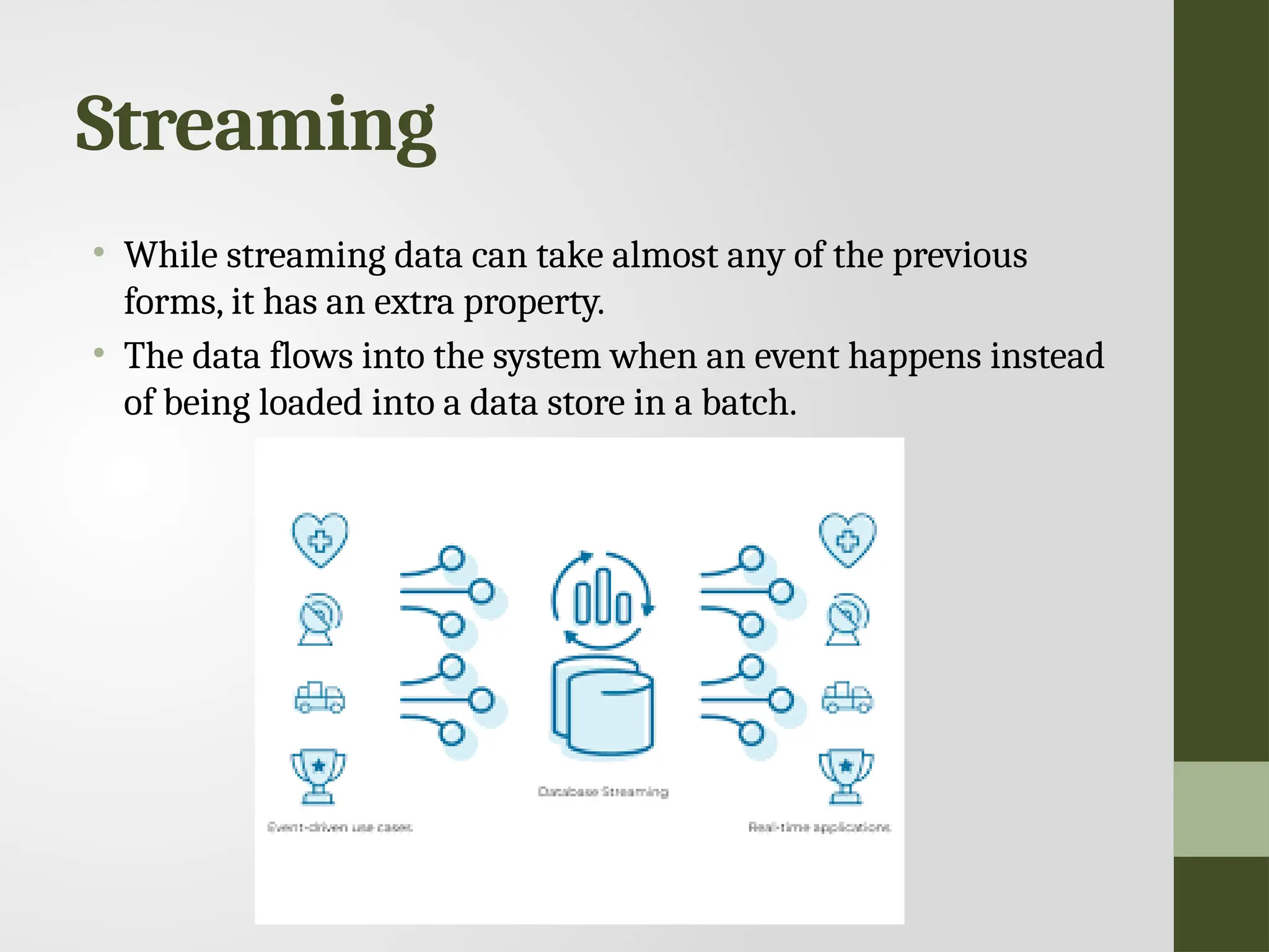
Streaming • While streamingdata can take almost any of the previous forms, it has an extra property. • The data flows into the system when an event happens instead of being loaded into a data store in a batch.
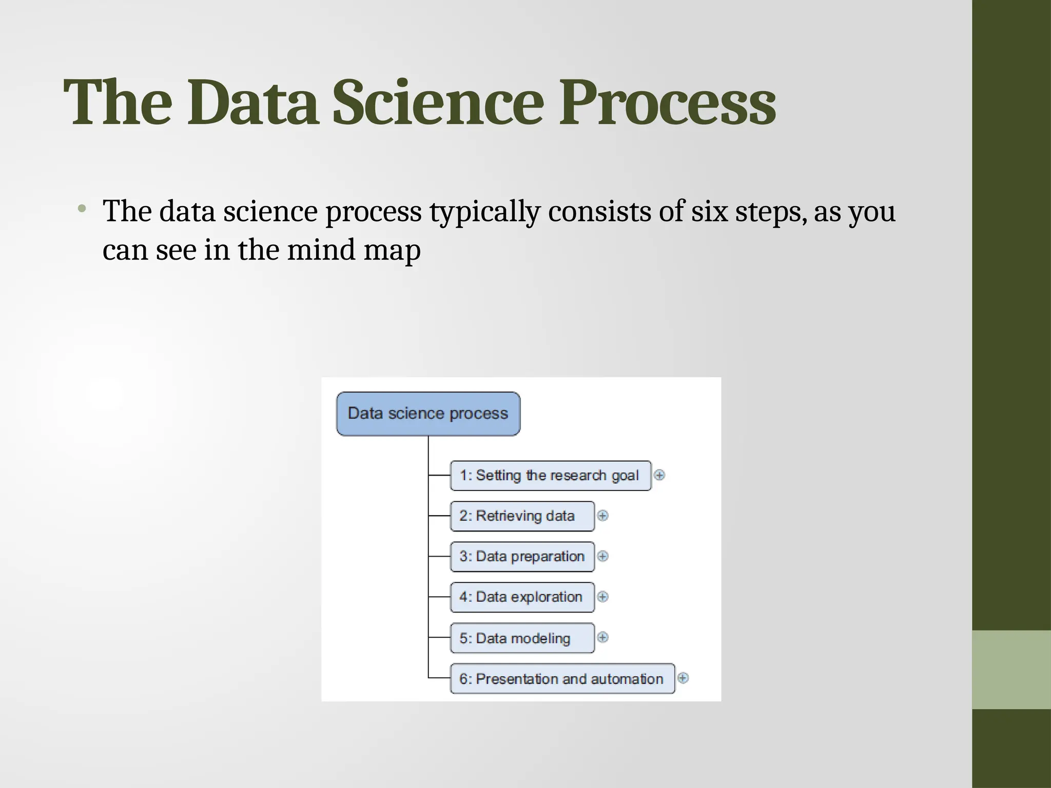
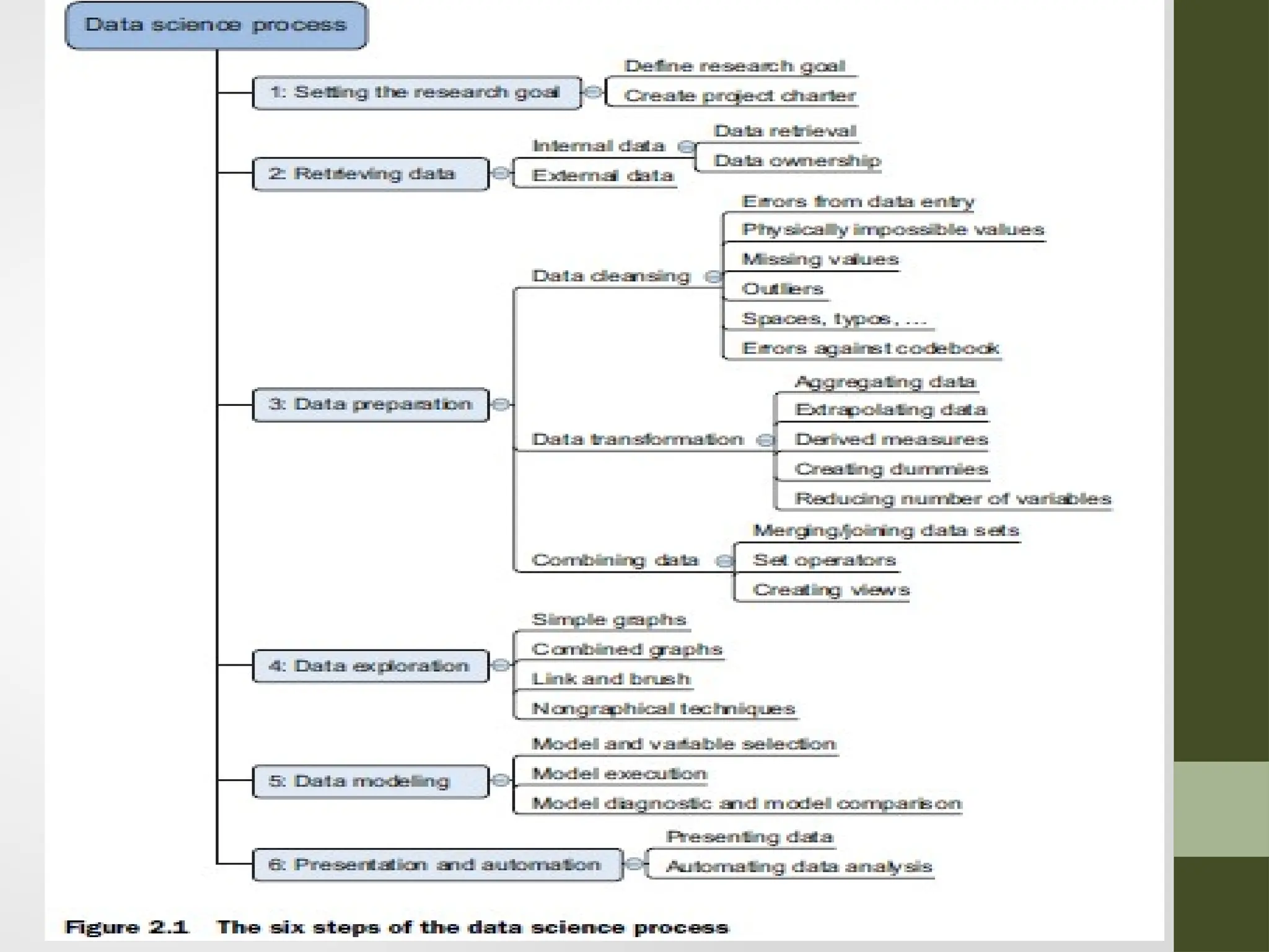
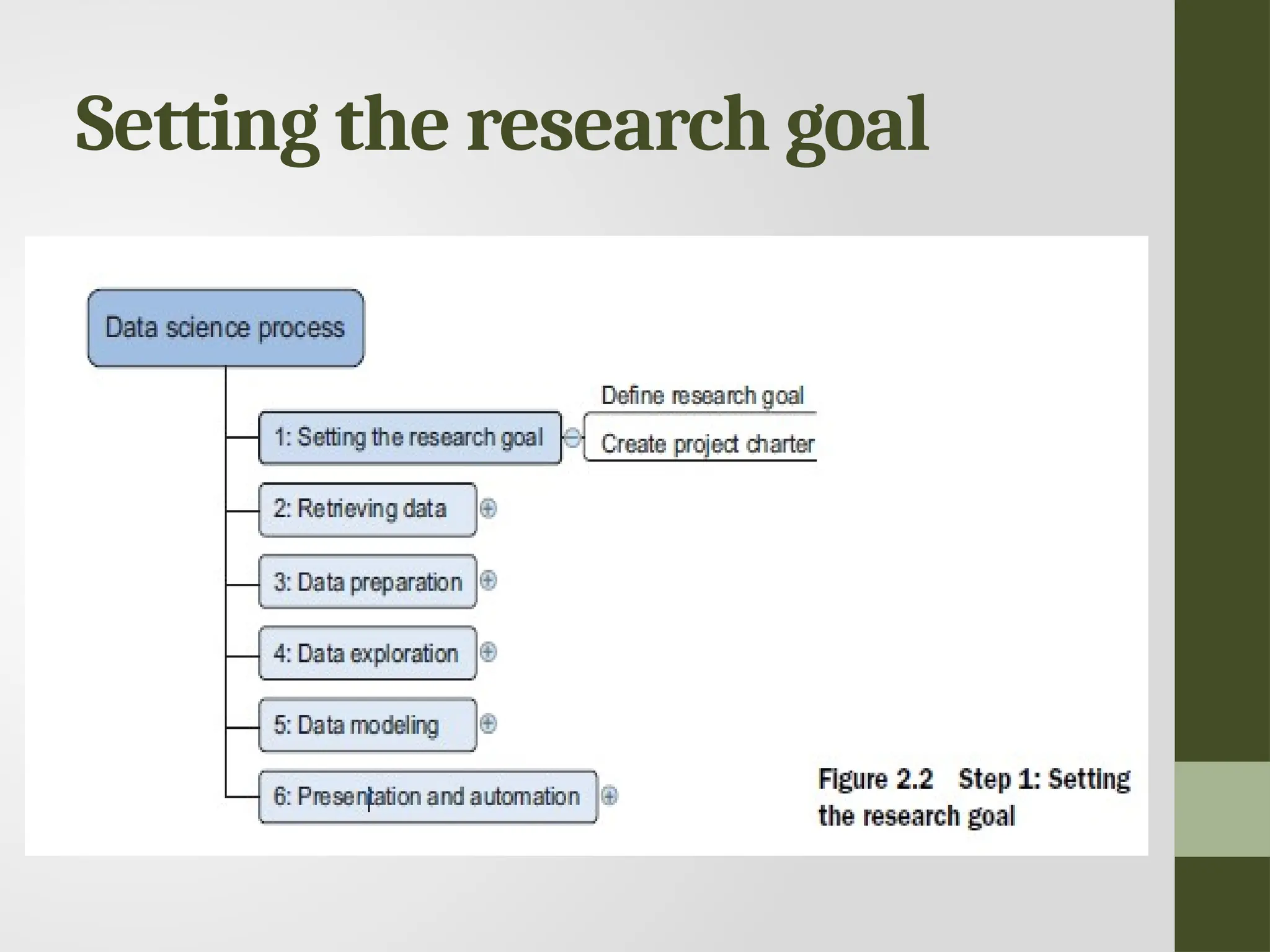
Setting the researchgoal • Data science is mostly applied in the context of an organization. • A clear research goal • The project mission and context • How you’re going to perform your analysis • What resources you expect to use • Proof that it’s an achievable project, or proof of concepts • Deliverables and a measure of success • A timeline
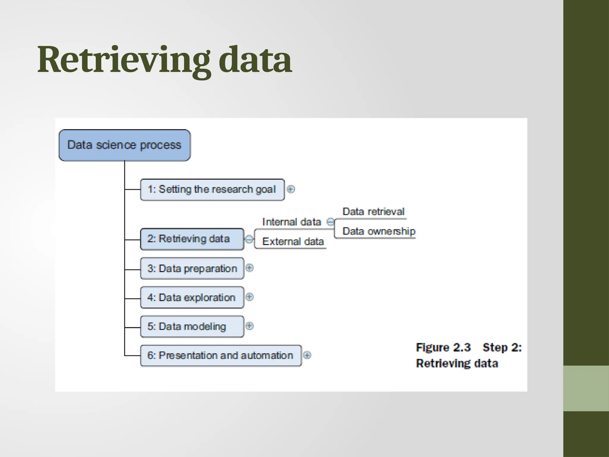
Retrieving data • Datacan be stored in many forms, ranging from simple text files to tables in a database. • The objective now is acquiring all the data you need. • Start with data stored within the company • Databases • Data marts • Data warehouses • Data lakes
23.
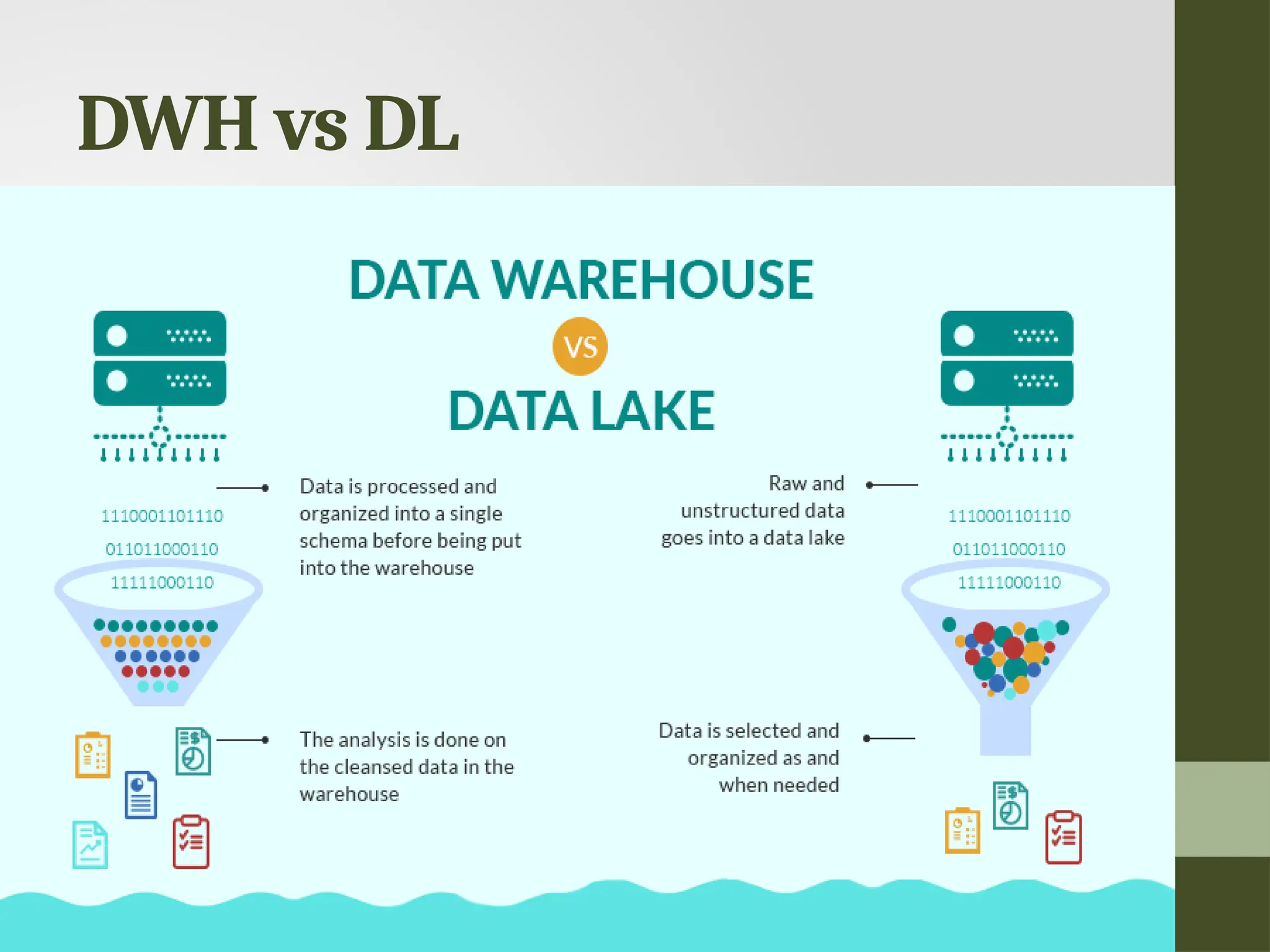
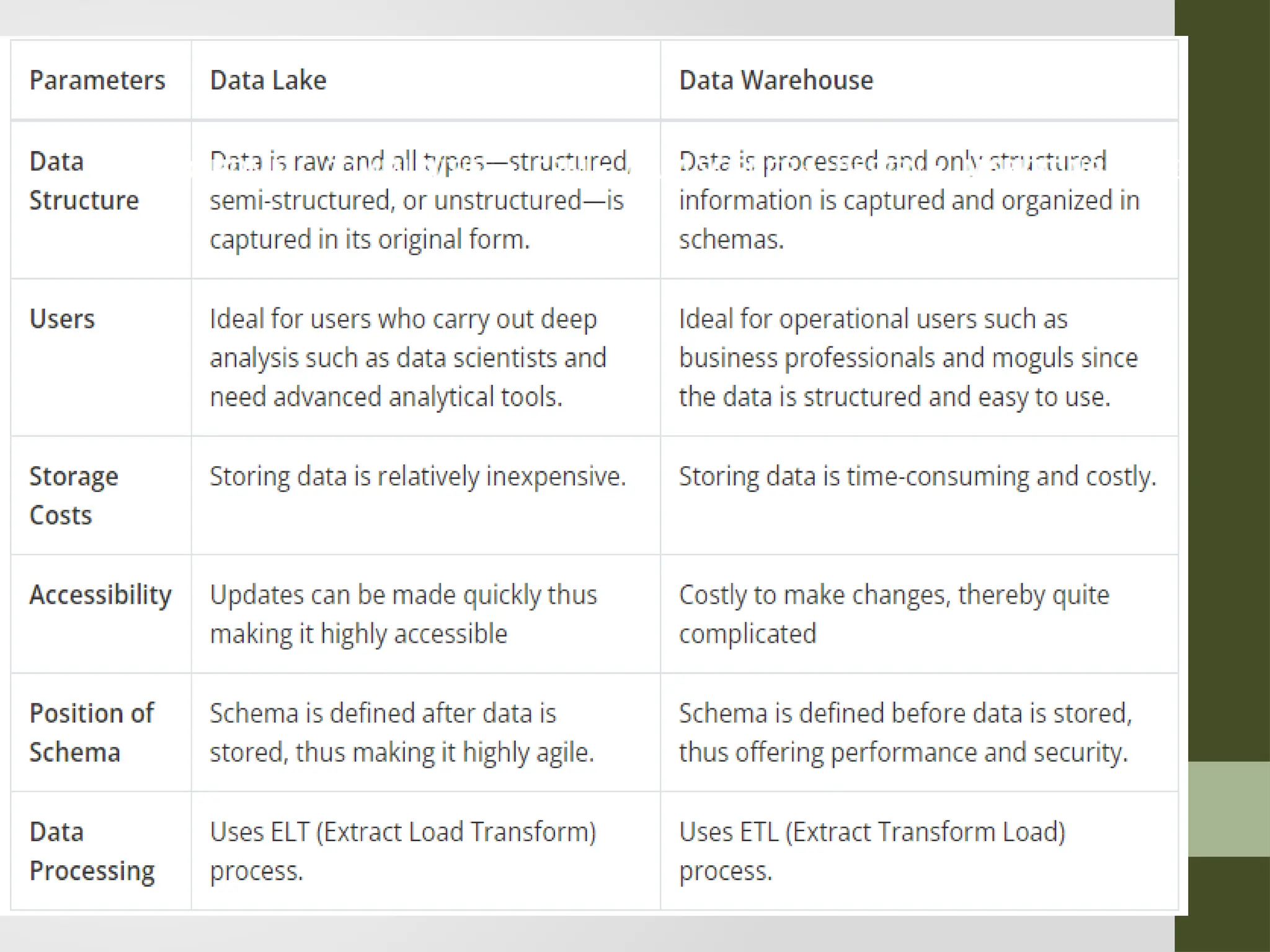
Data Lakes • Adata lake is a centralized storage repository that holds a massive amount of structured and unstructured data. • According to Gartner, “it is a collection of storage instances of various data assets additional to the originating data sources.”
24.
Data warehouse • Datawarehousing is about the collection of data from varied sources for meaningful business insights. • An electronic storage of a massive amount of information, it is a blend of technologies that enable the strategic use of data!
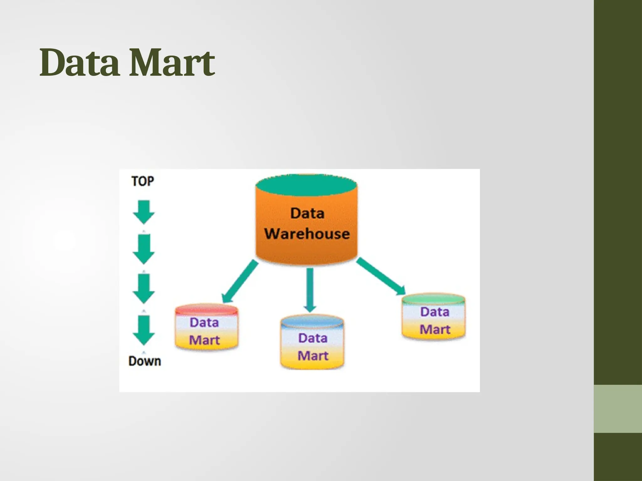
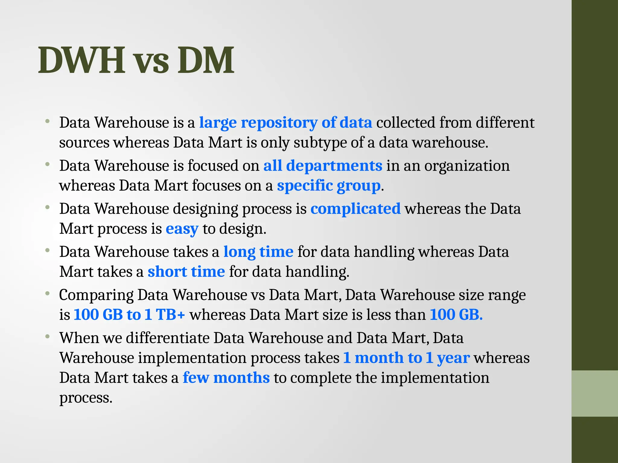
DWH vs DM •Data Warehouse is a large repository of data collected from different sources whereas Data Mart is only subtype of a data warehouse. • Data Warehouse is focused on all departments in an organization whereas Data Mart focuses on a specific group. • Data Warehouse designing process is complicated whereas the Data Mart process is easy to design. • Data Warehouse takes a long time for data handling whereas Data Mart takes a short time for data handling. • Comparing Data Warehouse vs Data Mart, Data Warehouse size range is 100 GB to 1 TB+ whereas Data Mart size is less than 100 GB. • When we differentiate Data Warehouse and Data Mart, Data Warehouse implementation process takes 1 month to 1 year whereas Data Mart takes a few months to complete the implementation process.
Data Lakes • Datalakes are a fairly new concept and experts have predicted that it might cause the death of data warehouses and data marts. • Although with the increase of unstructured data, data lakes will become quite popular. But you will probably prefer keeping your structured data in a data warehouse.
Cleansing data • Datacleansing is a sub process of the data science process that focuses on removing errors in your data so your data becomes a true and consistent representation of the processes it originates from. • True and consistent representation • interpretation error • inconsistencies
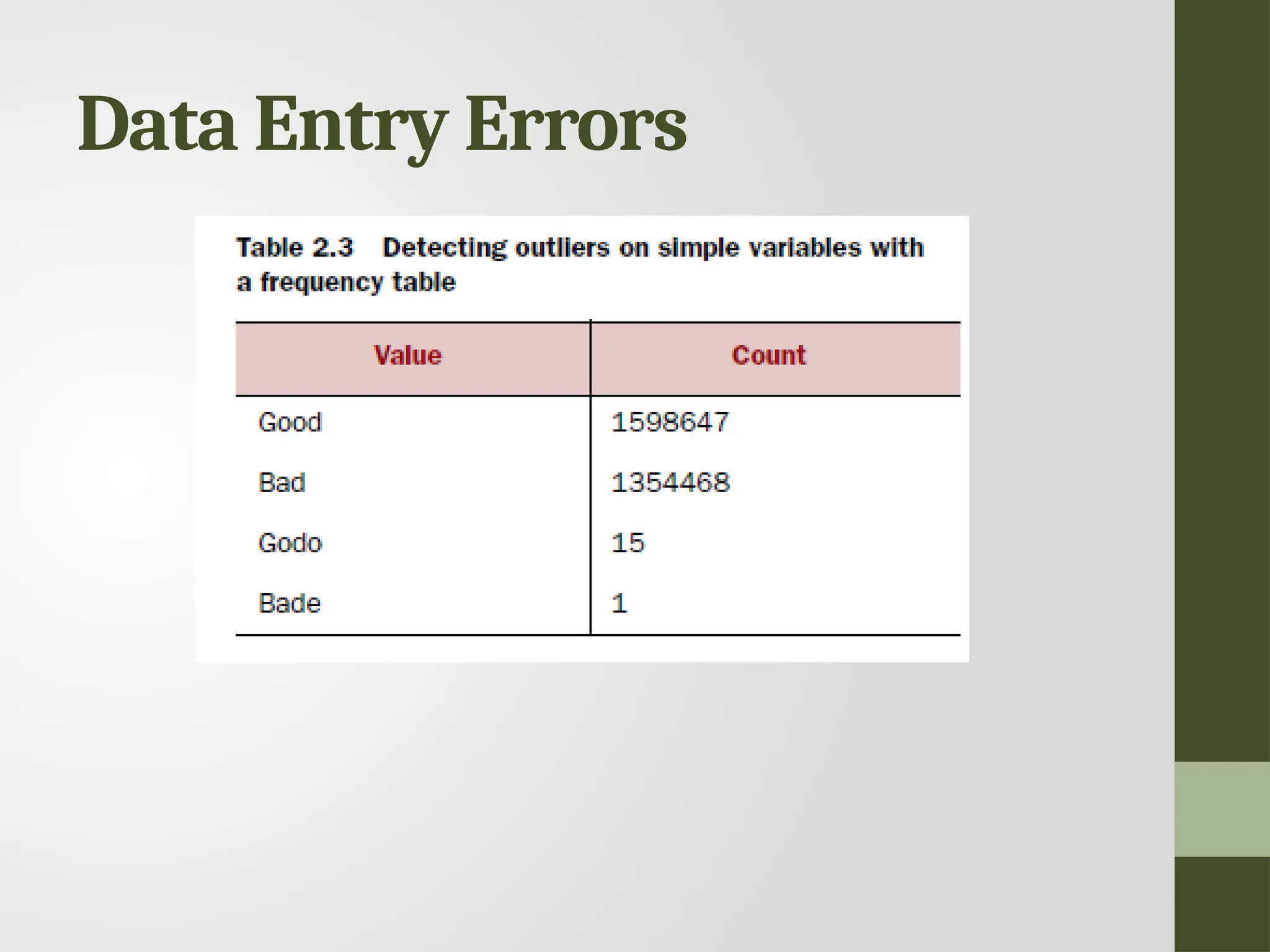
Data Entry Errors •Data collection and data entry are error-prone processes. • They often require human intervention, and because humans are only human, they make typos or lose their concentration for a second and introduce an error into the chain. But data collected by machines or computers isn’t free from errors either. • Errors can arise from human sloppiness, whereas others are due to machine or hardware failure.
Redundant Whitespaces • Whitespacestend to be hard to detect but cause errors like other redundant characters would. • Capital letter mismatches are common. • Most programming languages make a distinction between “Brazil” and “brazil”. In this case you can solve the problem by applying a function that returns both strings in lowercase, such as .lower() in Python. “Brazil”.lower() == “brazil”.lower() should result in true.
37.
Impossible values andSanity checks • Sanity checks are another valuable type of data check. • Sanity checks can be directly expressed with rules: check = 0 <= age <= 120
38.
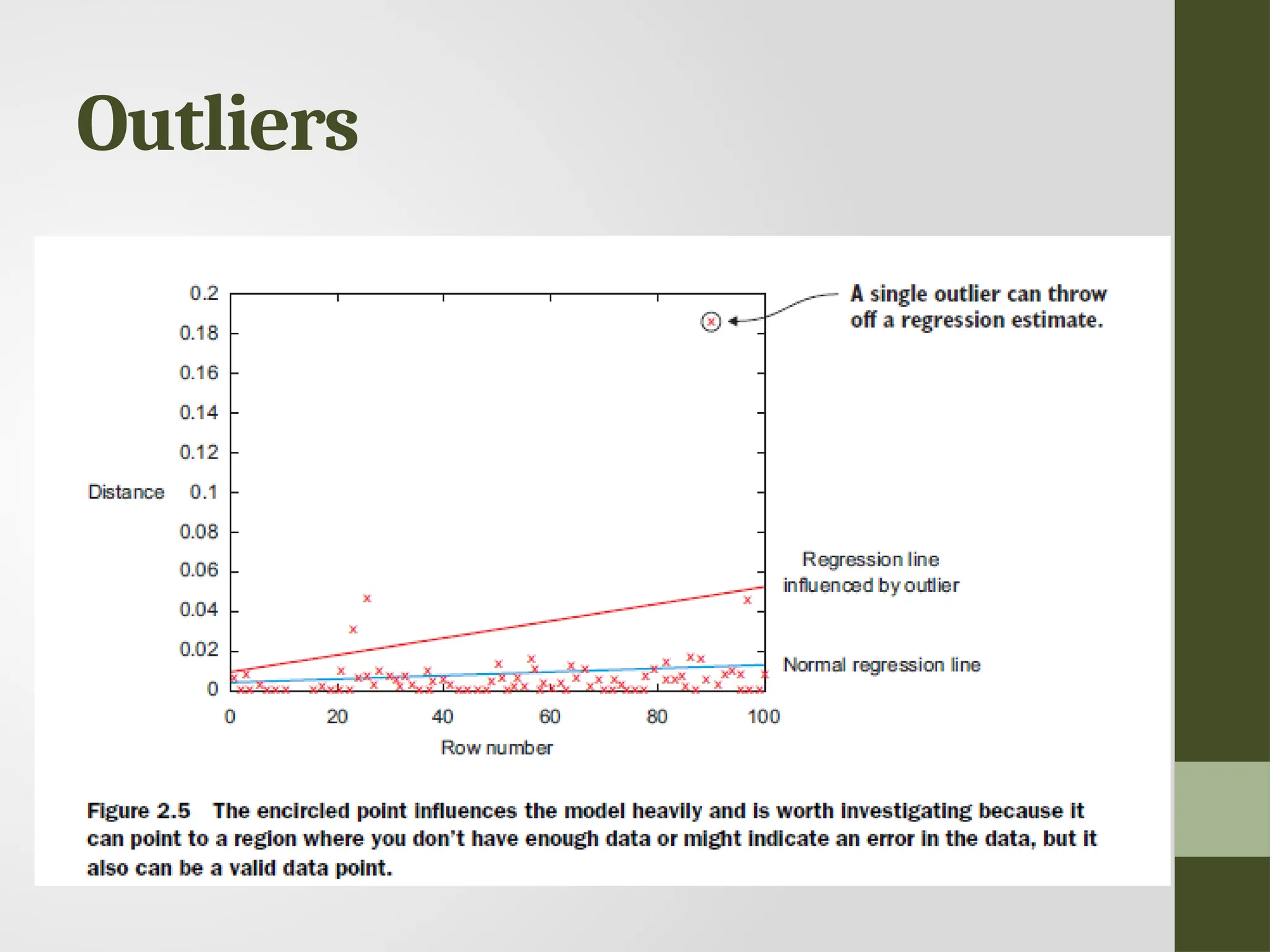
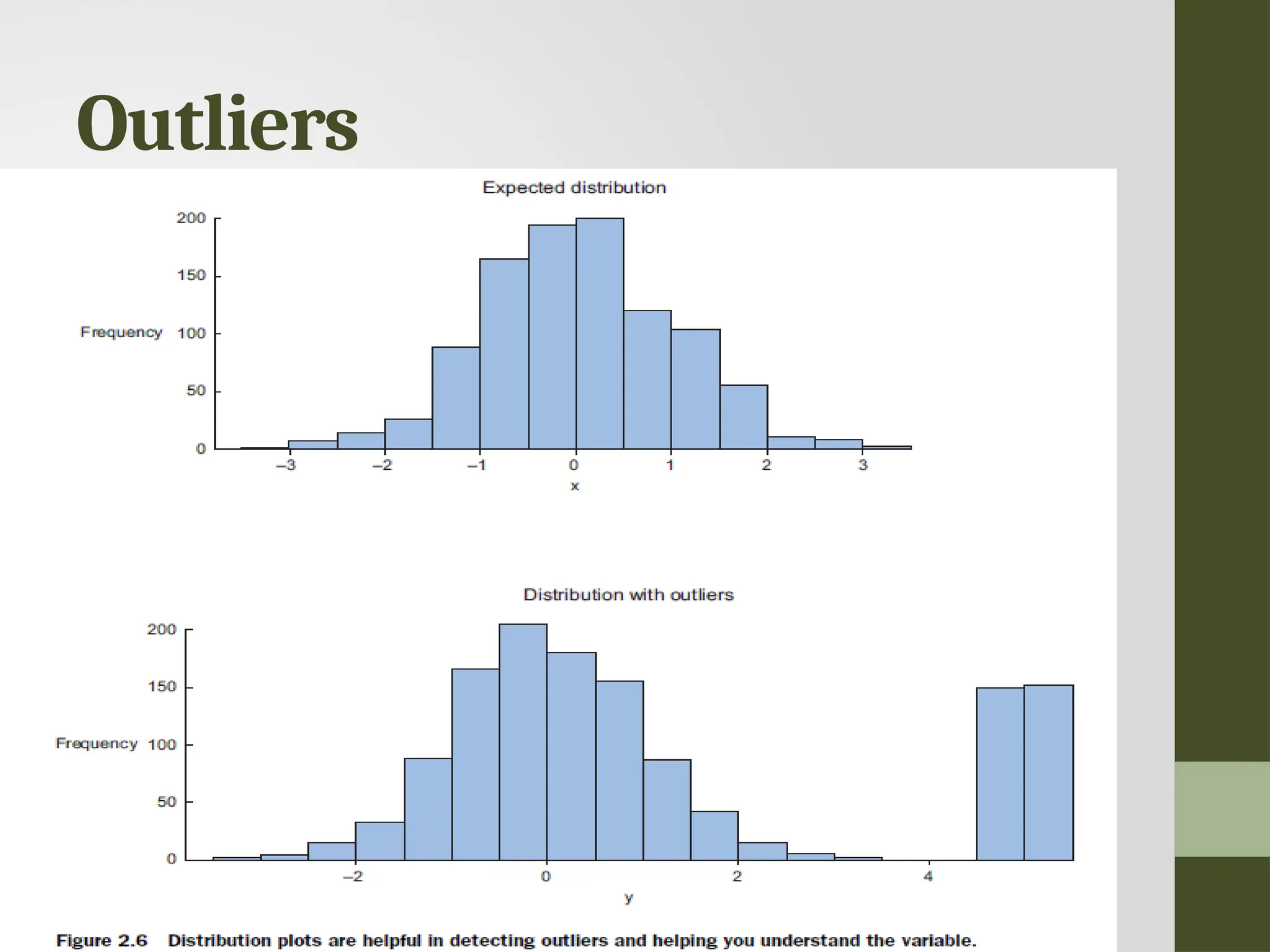
Outliers • An outlieris an observation that seems to be distant from other observations or, more specifically, one observation that follows a different logic or generative process than the other observations. • Find outliers Use a plot or table
Deviations from acode book • A code book is a description of your data, a form of metadata. • It contains things such as the number of variables per observation, the number of observations, and what each encoding within a variable means.(For instance “0” equals “negative”, “5” stands for “very positive”.)
42.
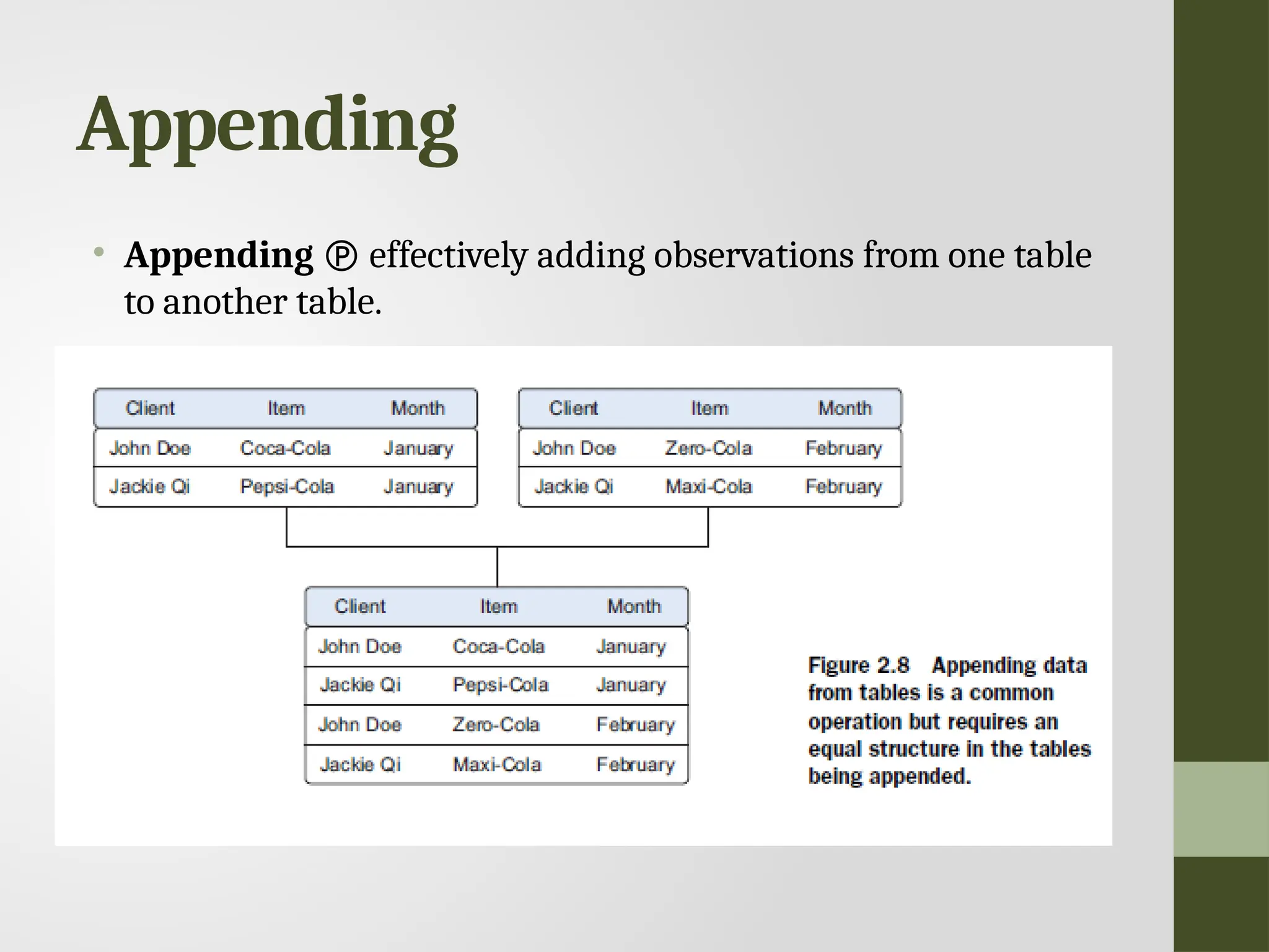
Combining data fromdifferent data sources • Joining enriching an observation from one table with information from another table • Appending or Stacking adding the observations of one table to those of another table.
43.
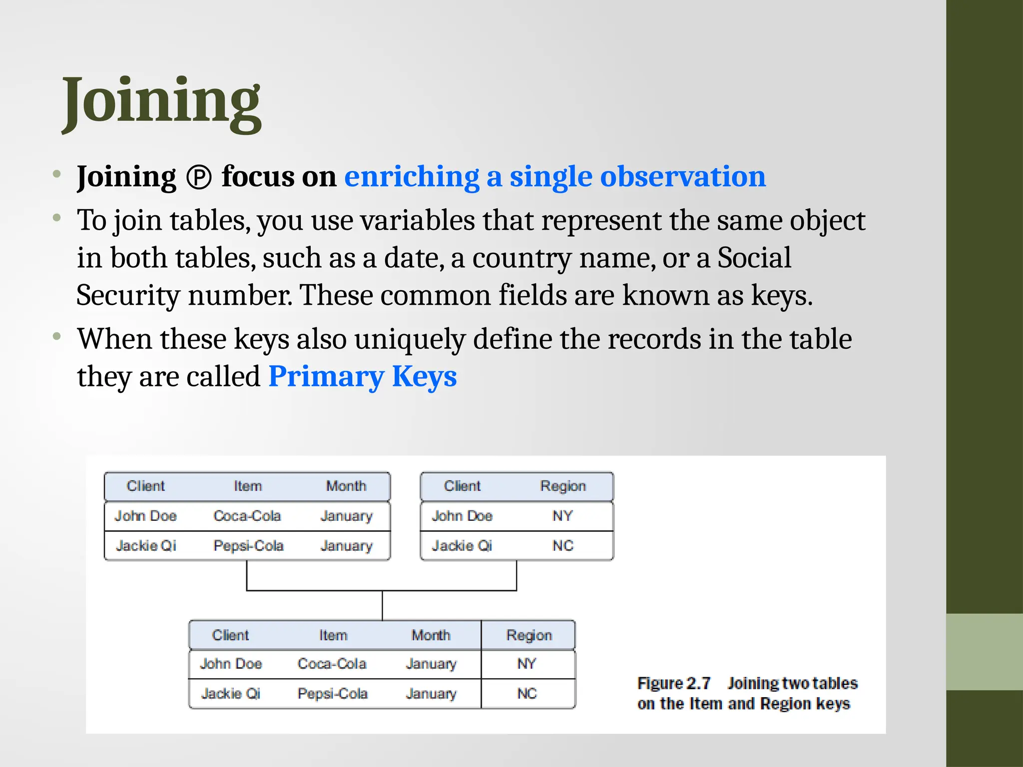
Joining • Joining focus on enriching a single observation • To join tables, you use variables that represent the same object in both tables, such as a date, a country name, or a Social Security number. These common fields are known as keys. • When these keys also uniquely define the records in the table they are called Primary Keys
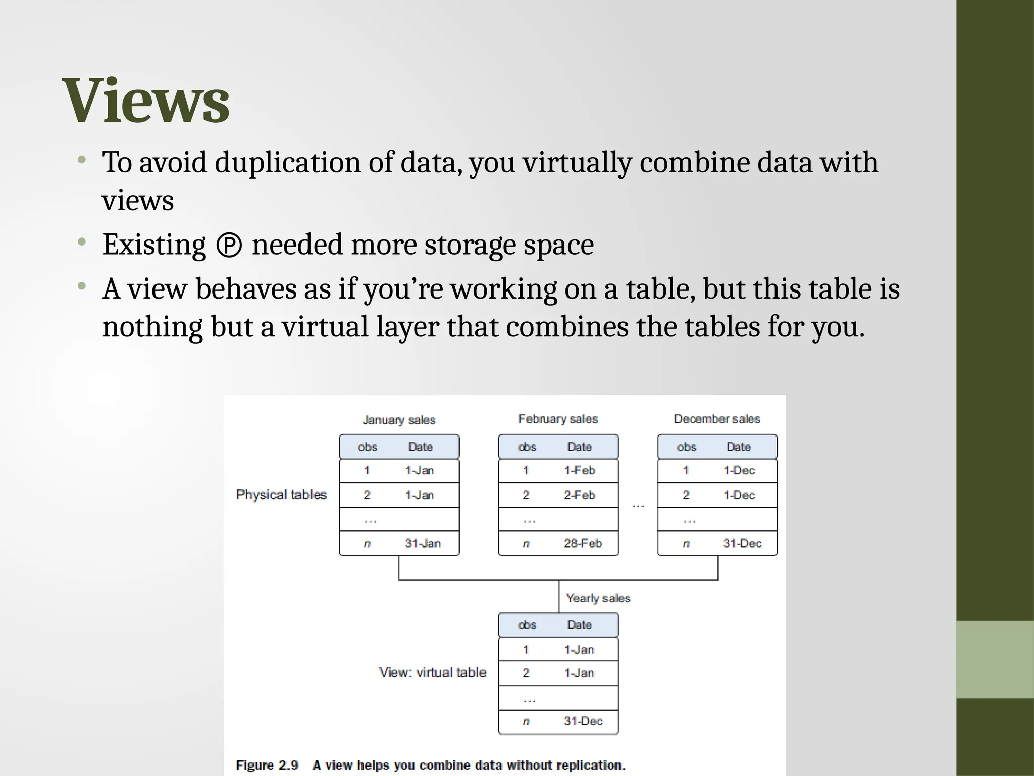
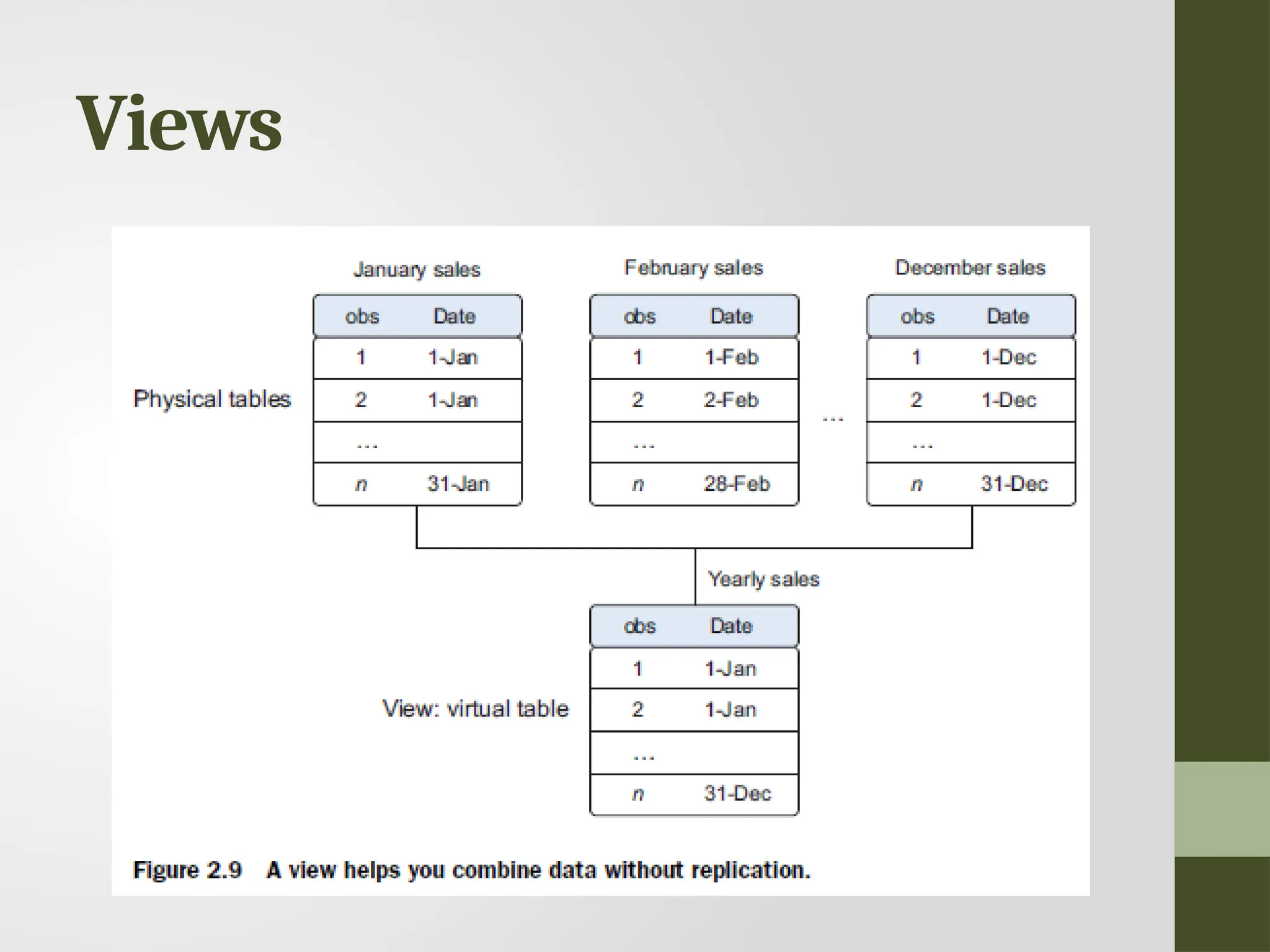
Views • To avoidduplication of data, you virtually combine data with views • Existing needed more storage space • A view behaves as if you’re working on a table, but this table is nothing but a virtual layer that combines the tables for you.
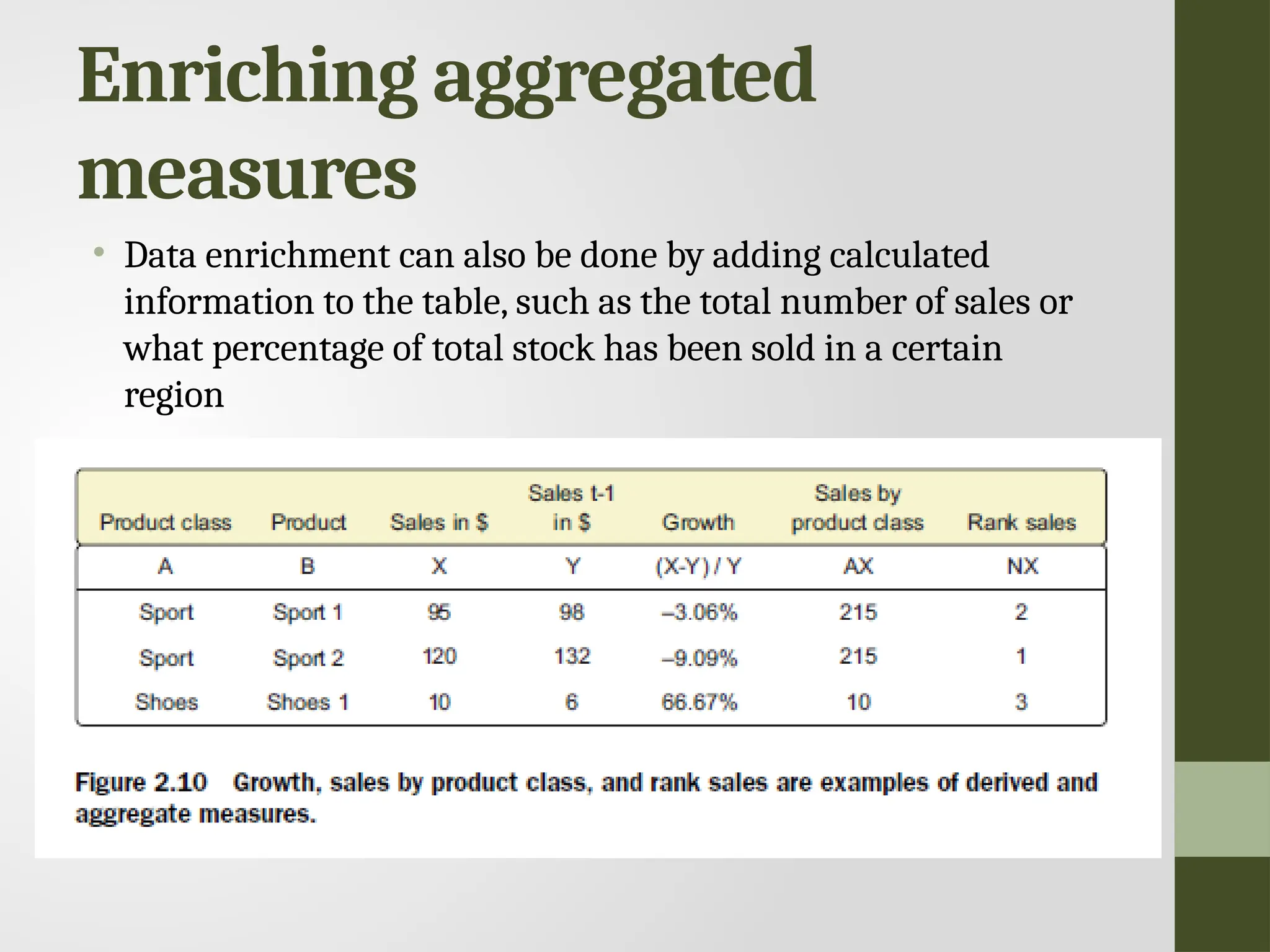
Enriching aggregated measures • Dataenrichment can also be done by adding calculated information to the table, such as the total number of sales or what percentage of total stock has been sold in a certain region
48.
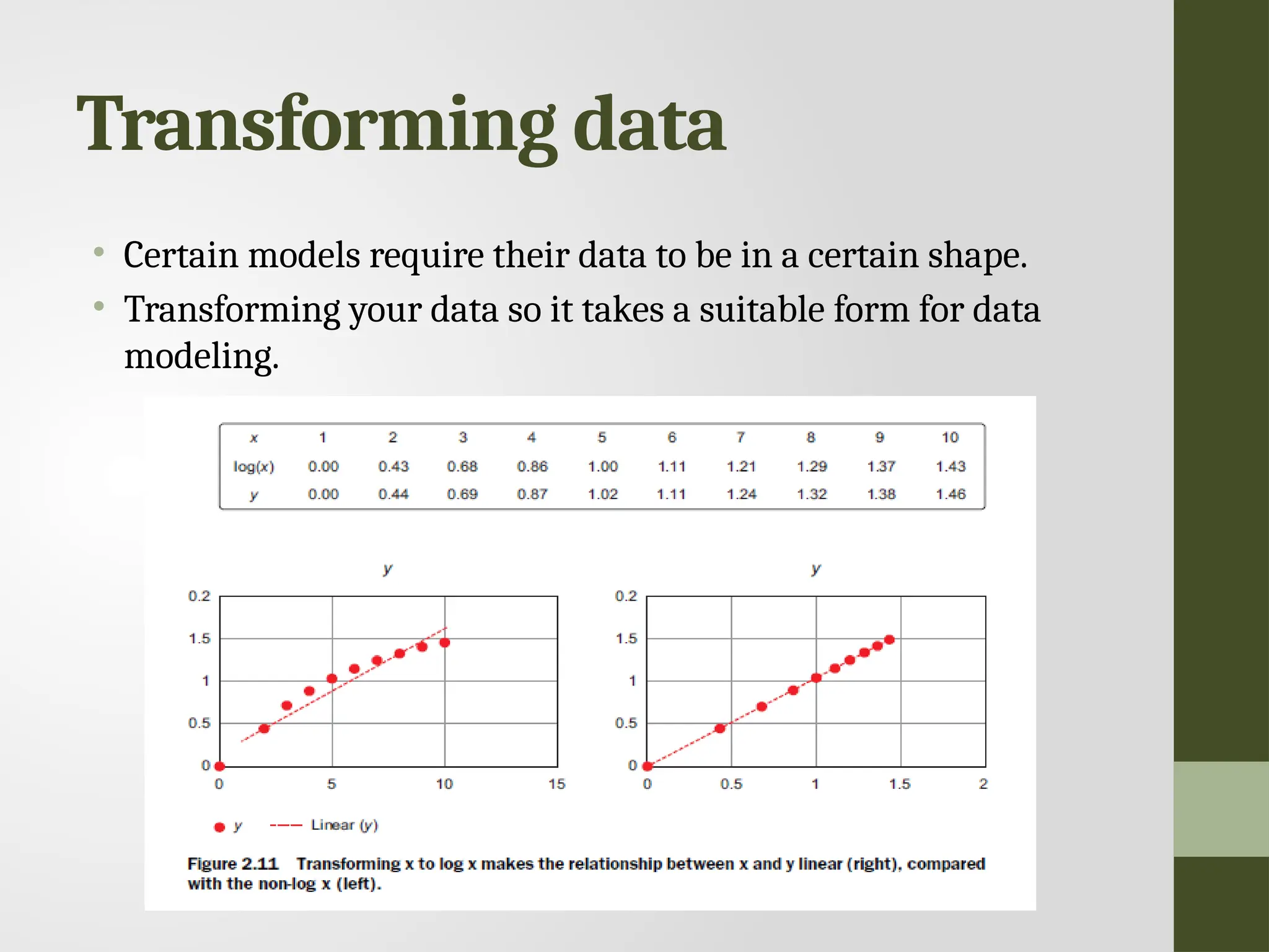
Transforming data • Certainmodels require their data to be in a certain shape. • Transforming your data so it takes a suitable form for data modeling.
49.
Reducing the numberof variables • Too many variables don’t add new information to the model model difficult to handle certain techniques don’t perform well when you overload them with too many input variables • Data scientists use special methods to reduce the number of variables but retain the maximum amount of data.
50.
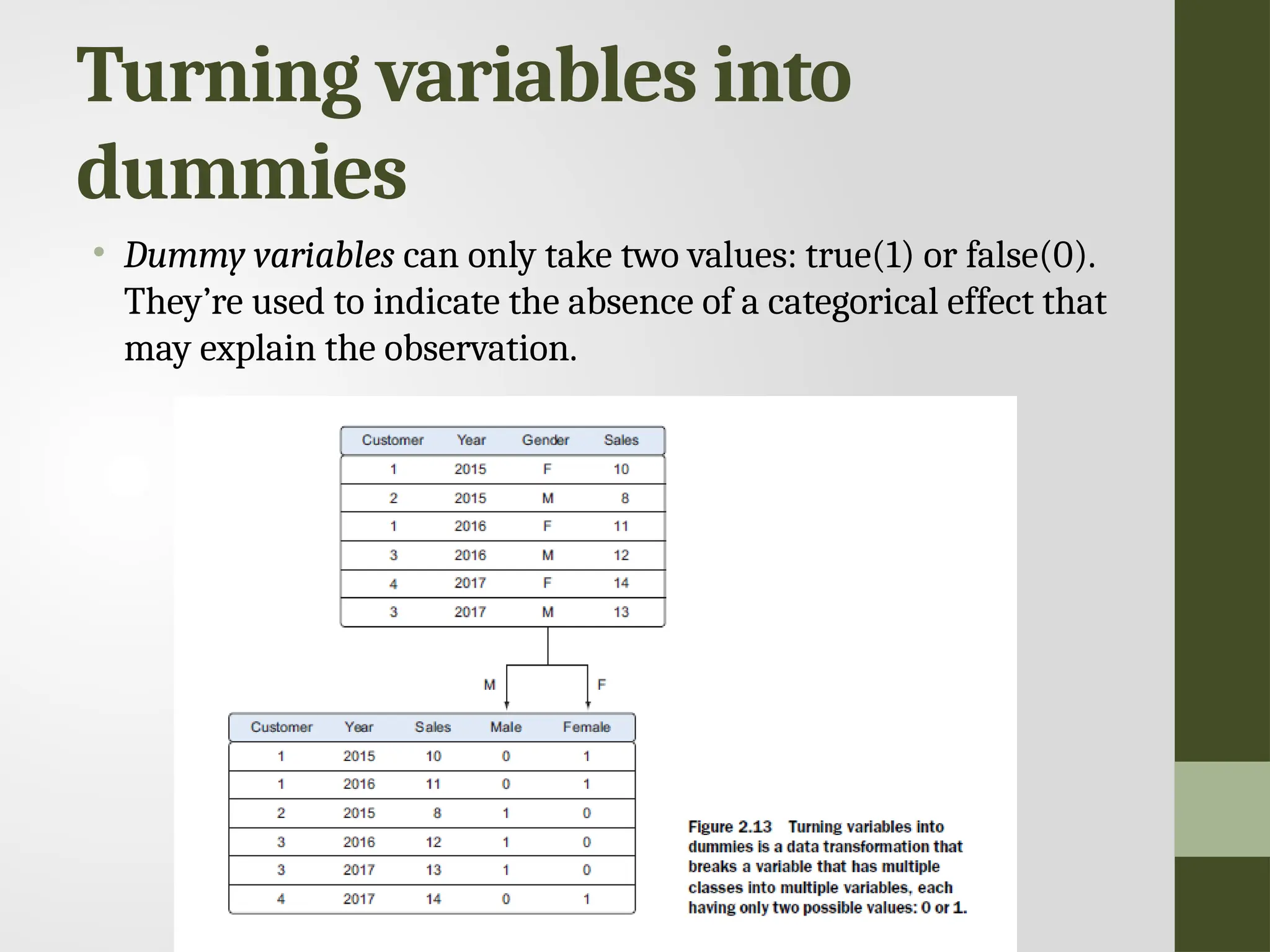
Turning variables into dummies •Dummy variables can only take two values: true(1) or false(0). They’re used to indicate the absence of a categorical effect that may explain the observation.
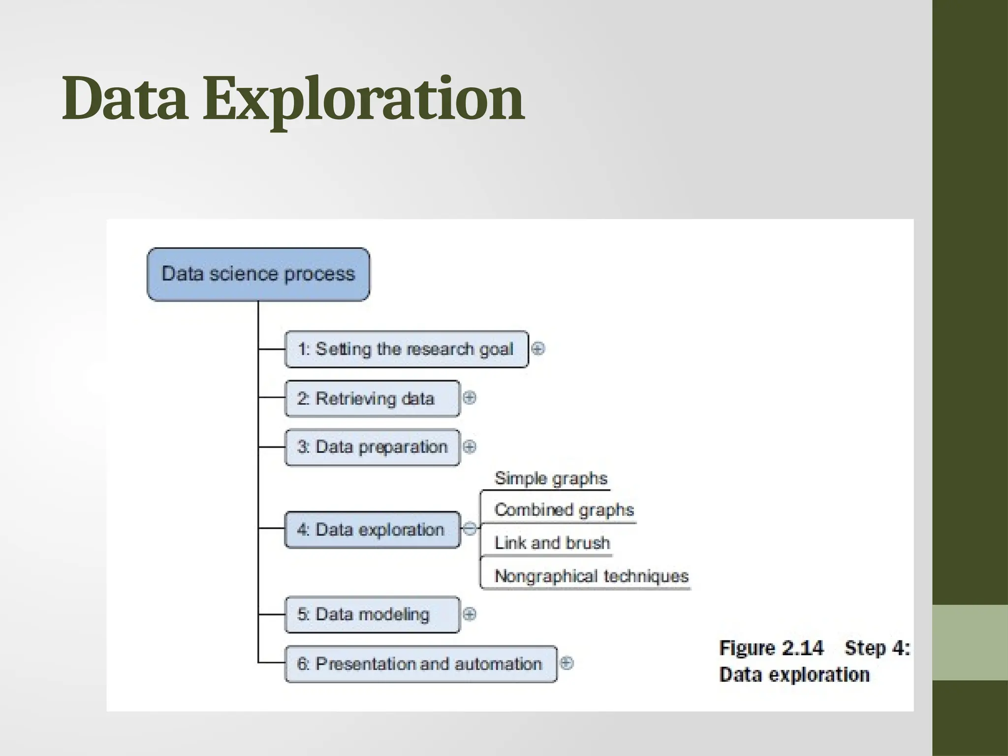
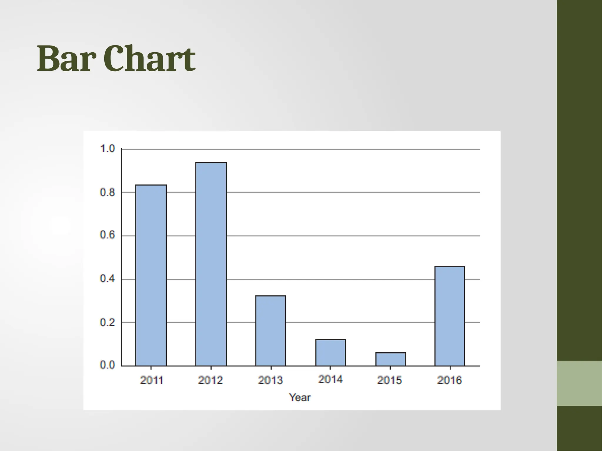
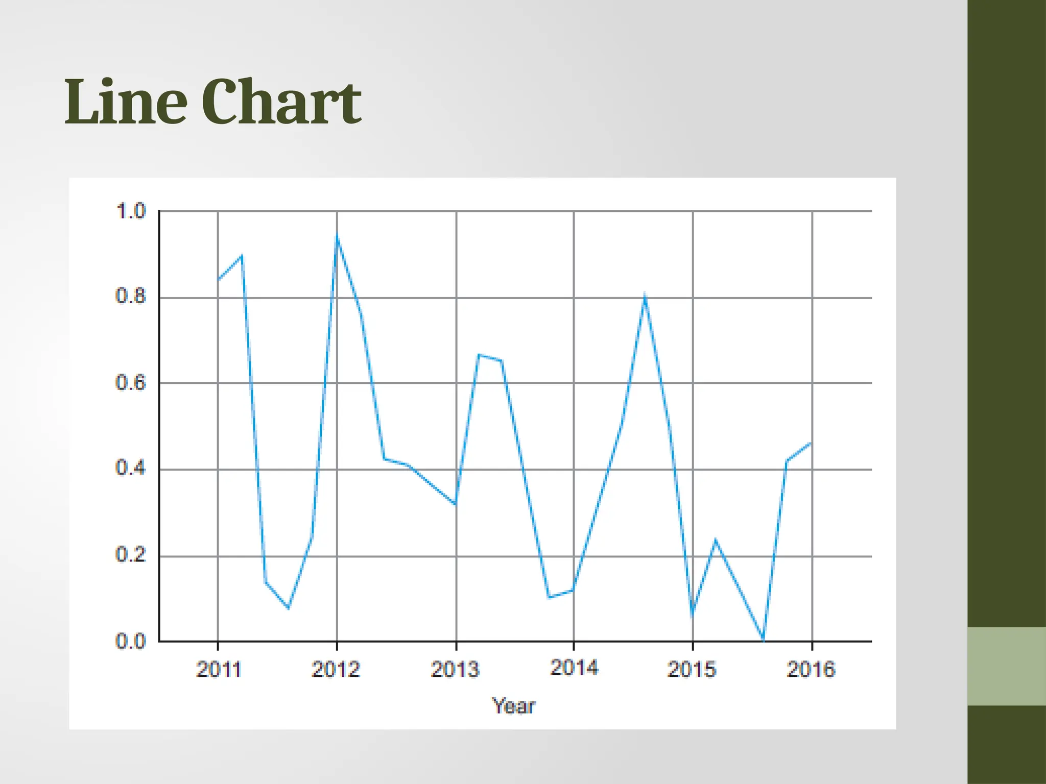
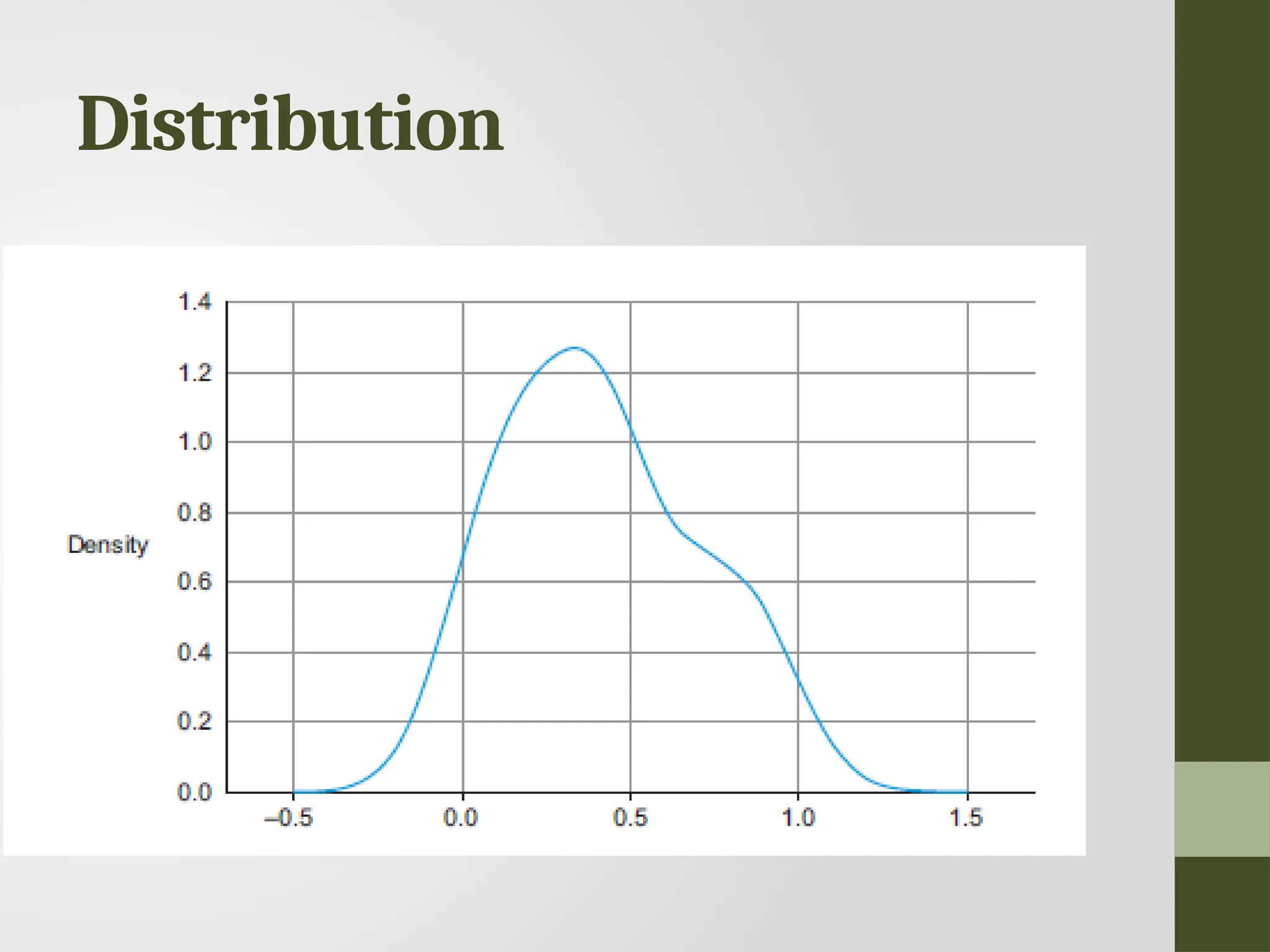
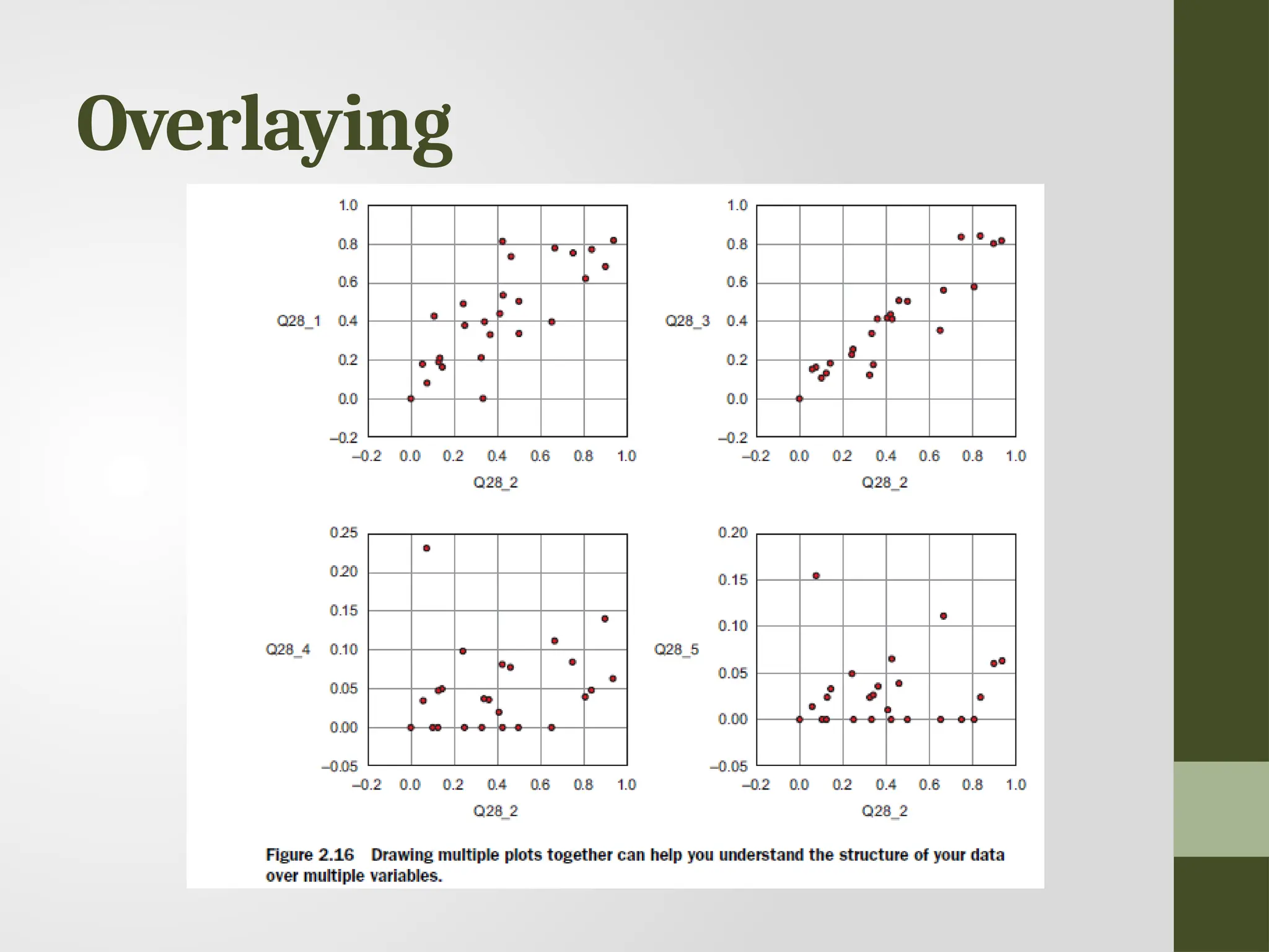
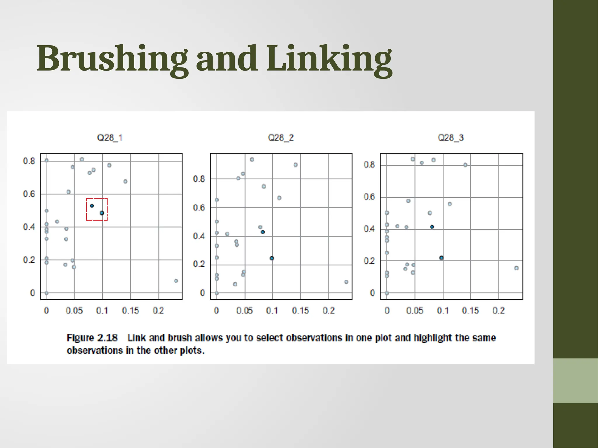
Data Exploration • Informationbecomes much easier to grasp when shown in a picture, therefore you mainly use graphical techniques to gain an understanding of your data and the interactions between variables. • Visualization Techniques • Simple graphs • Histograms • Sankey • Network graphs
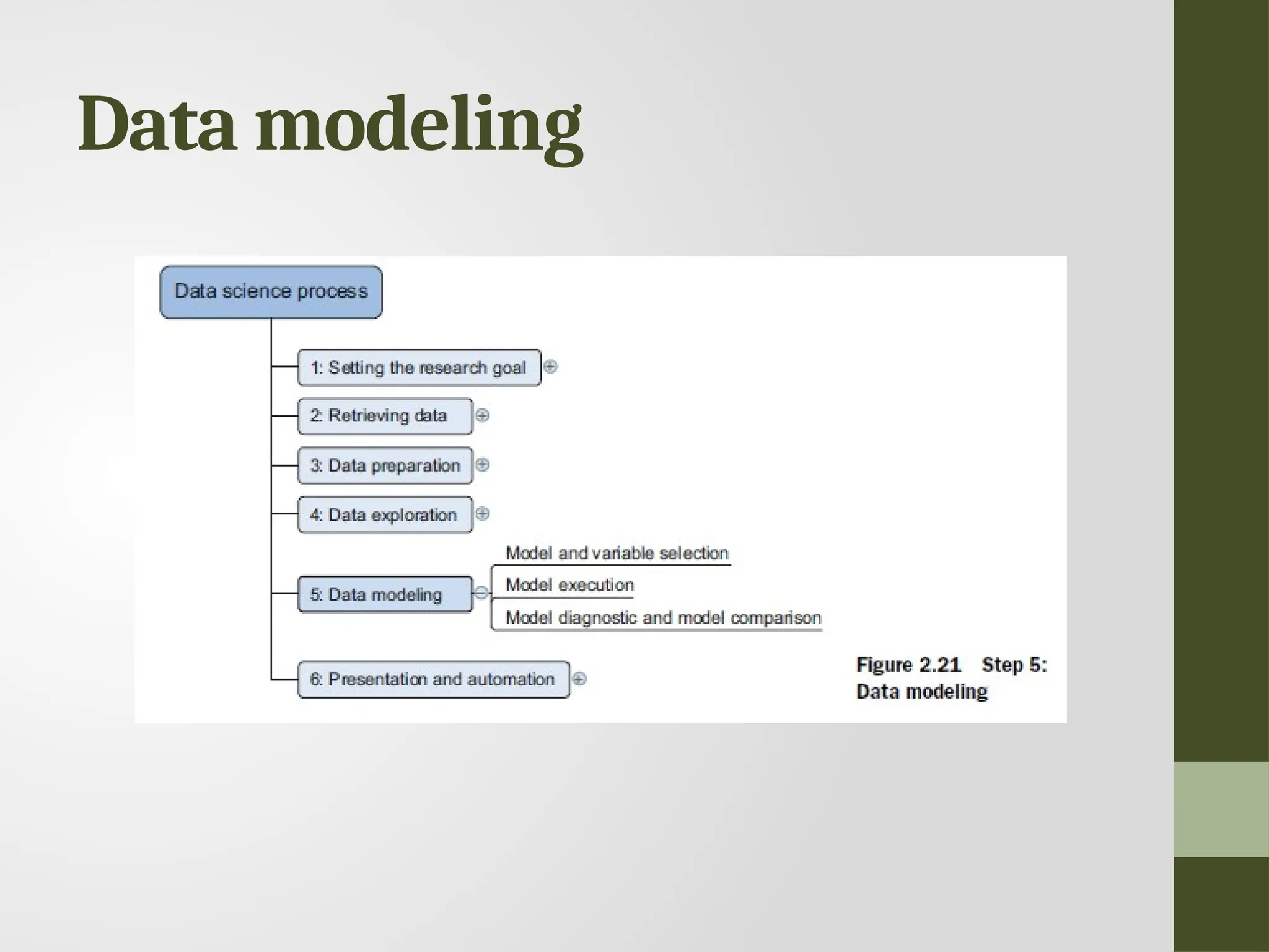
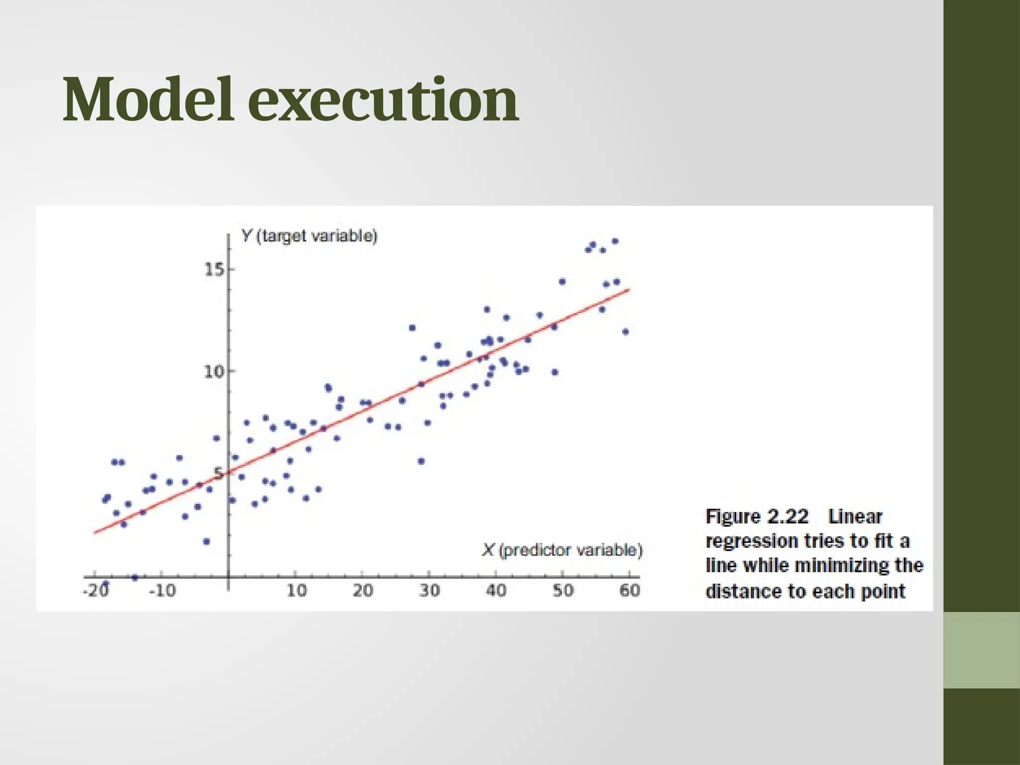
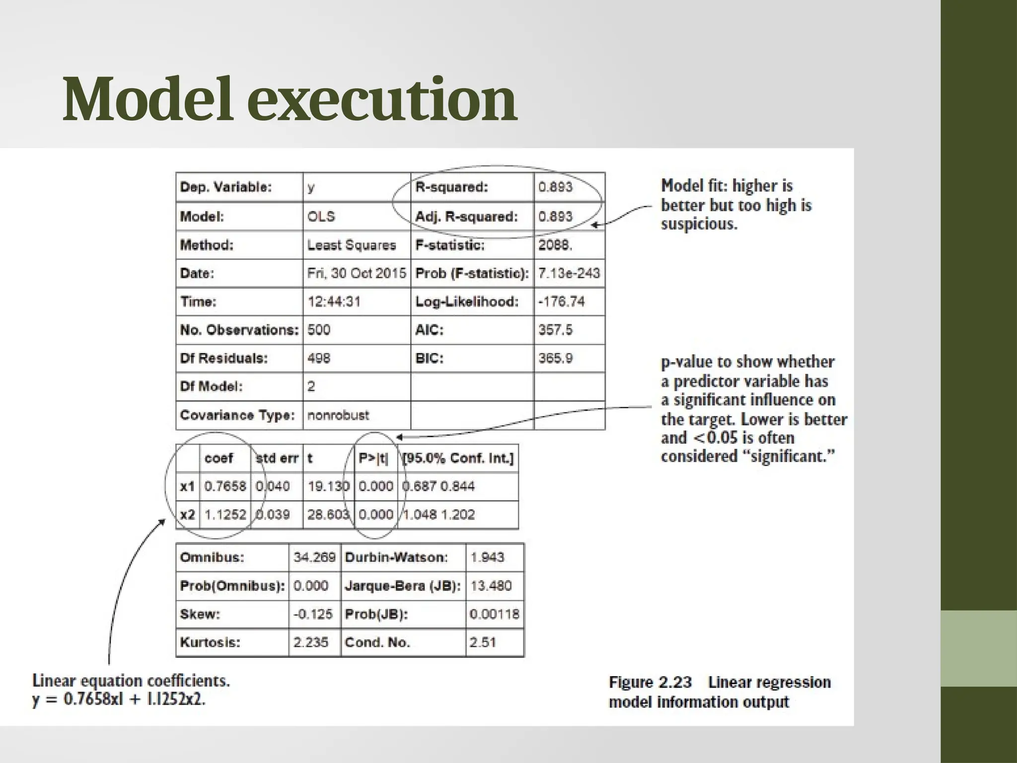
Data modeling • Buildinga model is an iterative process. • The way you build your model depends on whether you go with classic statistics or the somewhat more recent machine learning school, and the type of technique you want to use. • Models consist of the following main steps: • 1 Selection of a modeling technique and variables to enter in the model • 2 Execution of the model • 3 Diagnosis and model comparison
61.
Model and variableselection Must the model be moved to a production environment and, if so, would it be easy to implement? How difficult is the maintenance on the model: how long will it remain relevant if left untouched? Does the model need to be easy to explain?
NumPy • Numerical Python •General-purpose array-processing package. • High-performance multidimensional array object, and tools for working with these arrays. • Fundamental package for scientific computing with Python. • It is open-source software.
68.
NumPy - Features •A powerful N-dimensional array object • Sophisticated (broadcasting) functions • Tools for integrating C/C++ and Fortran code • Useful linear algebra, Fourier transform, and random number capabilities
Array • An arrayis a data type used to store multiple values using a single identifier (variable name). • An array contains an ordered collection of data elements where each element is of the same type and can be referenced by its index (position)
71.
Array • Similar tothe indexing of lists • Zero-based indexing • [10, 9, 99, 71, 90 ]
72.
NumPy Array • Storelists of numerical data, vectors and matrices • Large set of routines (built-in functions) for creating, manipulating, and transforming NumPy arrays. • NumPy array is officially called ndarray but commonly known as array
73.
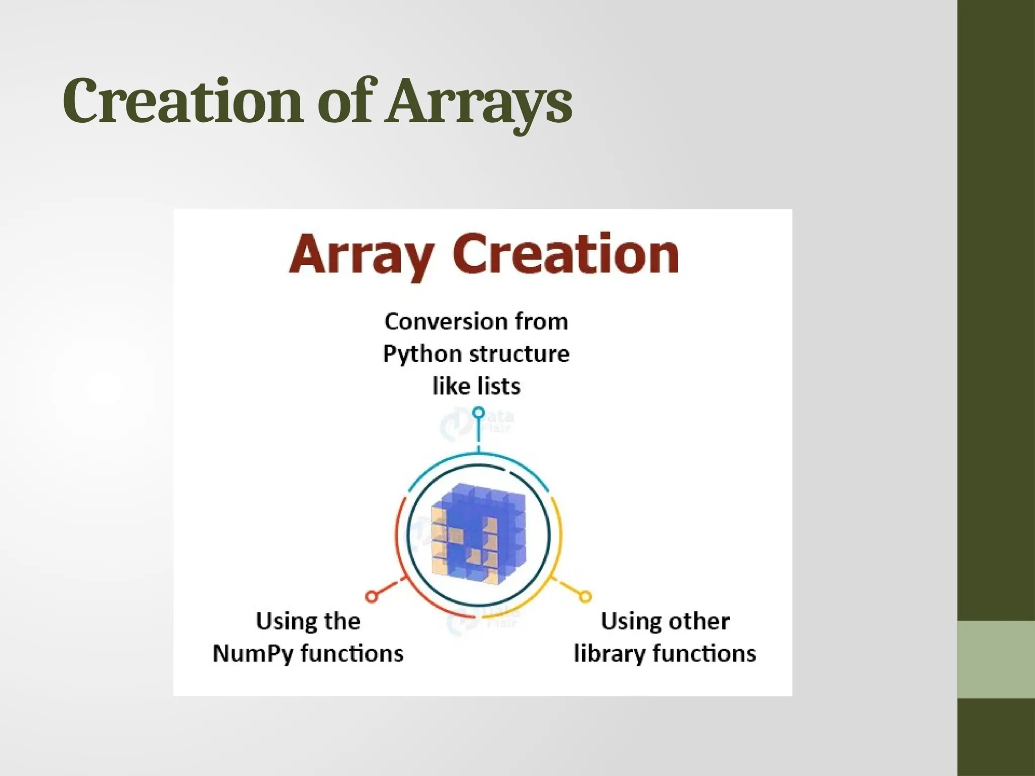
Creation of NumPyArrays from List • First we need to import the NumPy library import numpy as np
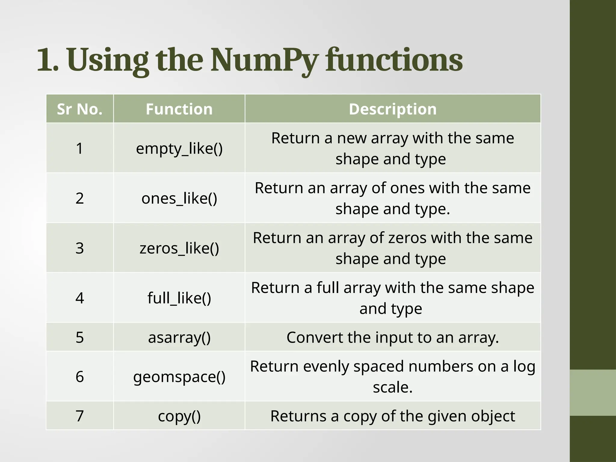
1. Using theNumPy functions Sr No. Function Description 1 empty_like() Return a new array with the same shape and type 2 ones_like() Return an array of ones with the same shape and type. 3 zeros_like() Return an array of zeros with the same shape and type 4 full_like() Return a full array with the same shape and type 5 asarray() Convert the input to an array. 6 geomspace() Return evenly spaced numbers on a log scale. 7 copy() Returns a copy of the given object
83.
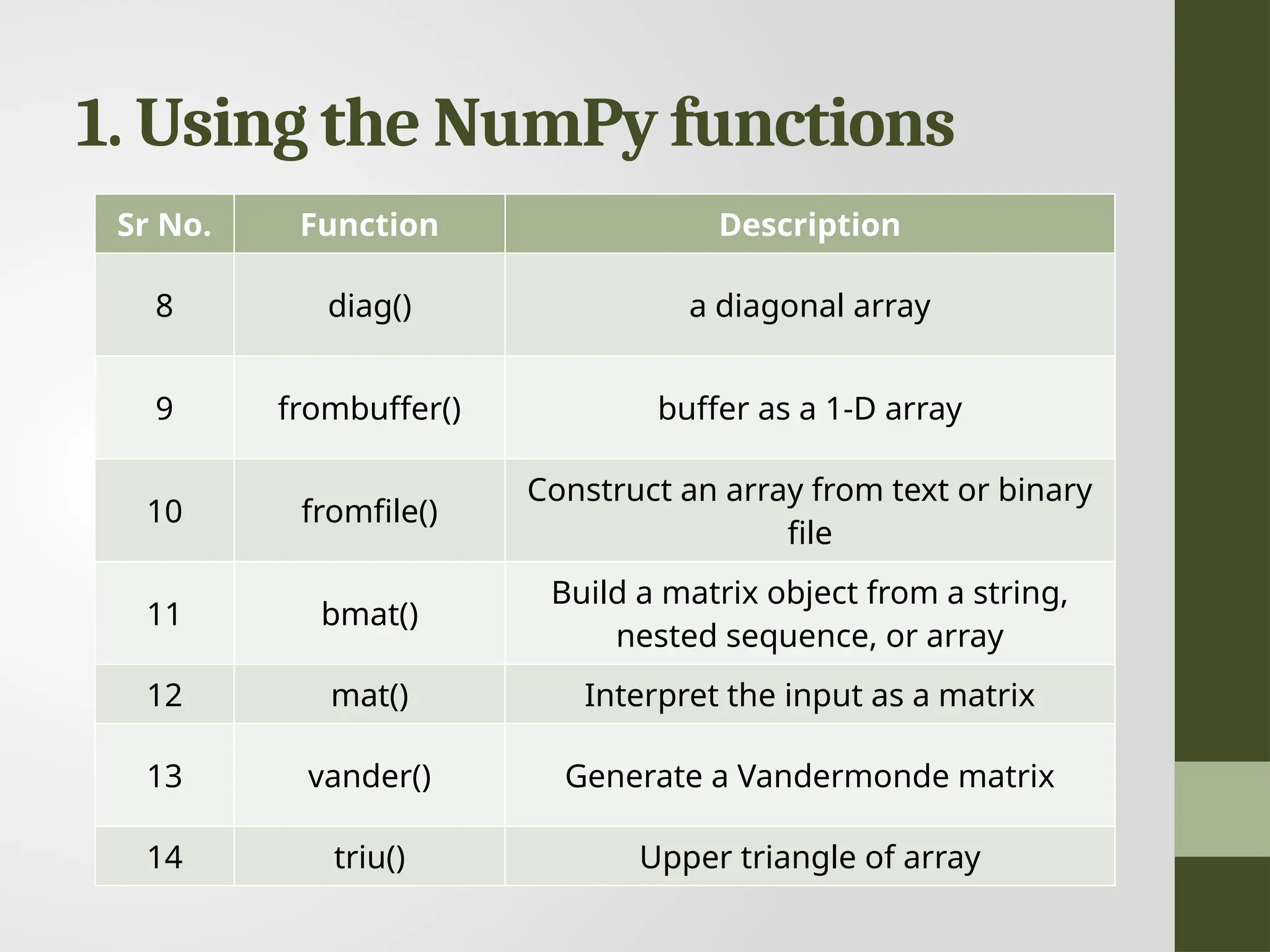
1. Using theNumPy functions Sr No. Function Description 8 diag() a diagonal array 9 frombuffer() buffer as a 1-D array 10 fromfile() Construct an array from text or binary file 11 bmat() Build a matrix object from a string, nested sequence, or array 12 mat() Interpret the input as a matrix 13 vander() Generate a Vandermonde matrix 14 triu() Upper triangle of array
84.
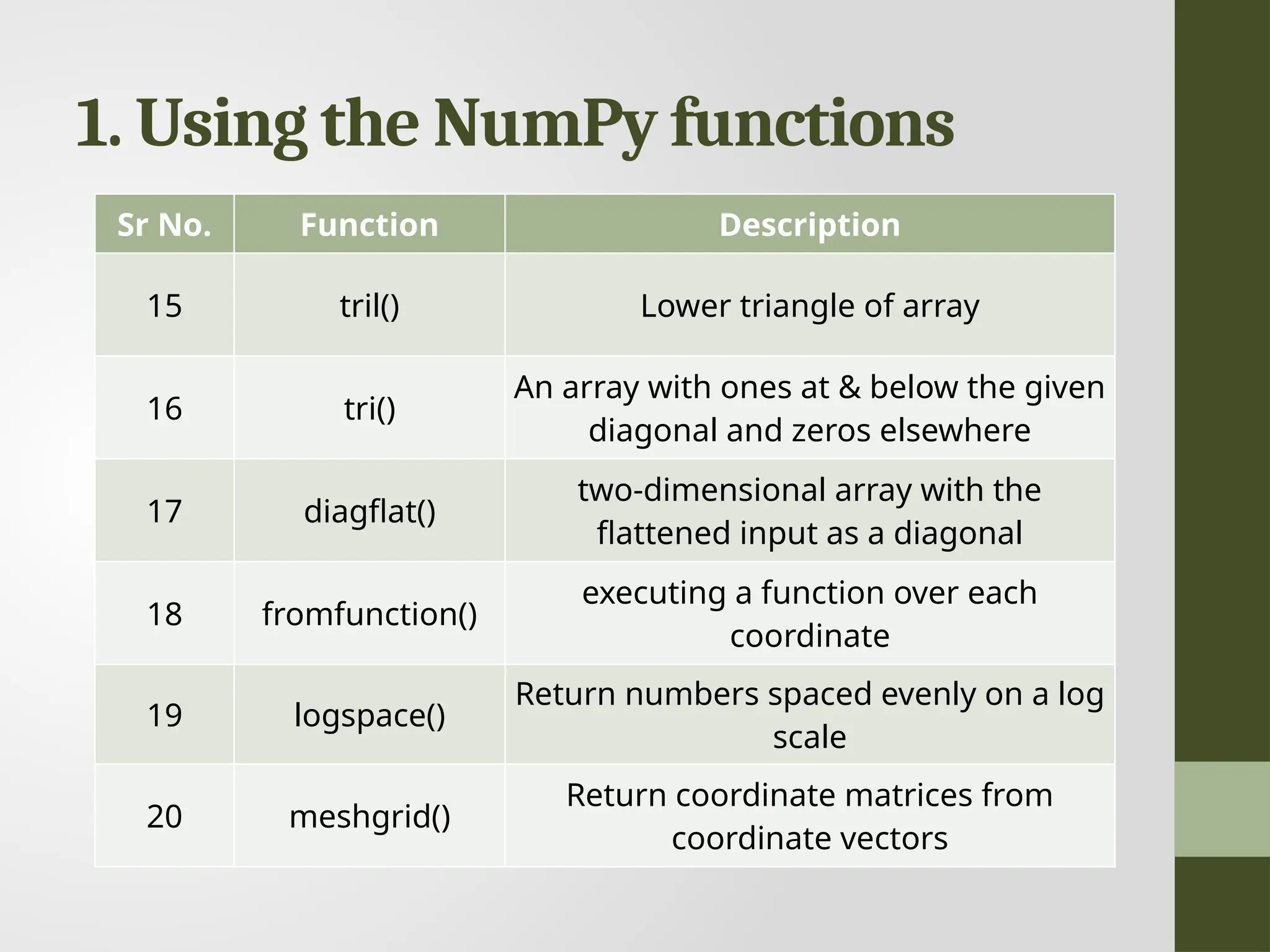
1. Using theNumPy functions Sr No. Function Description 15 tril() Lower triangle of array 16 tri() An array with ones at & below the given diagonal and zeros elsewhere 17 diagflat() two-dimensional array with the flattened input as a diagonal 18 fromfunction() executing a function over each coordinate 19 logspace() Return numbers spaced evenly on a log scale 20 meshgrid() Return coordinate matrices from coordinate vectors
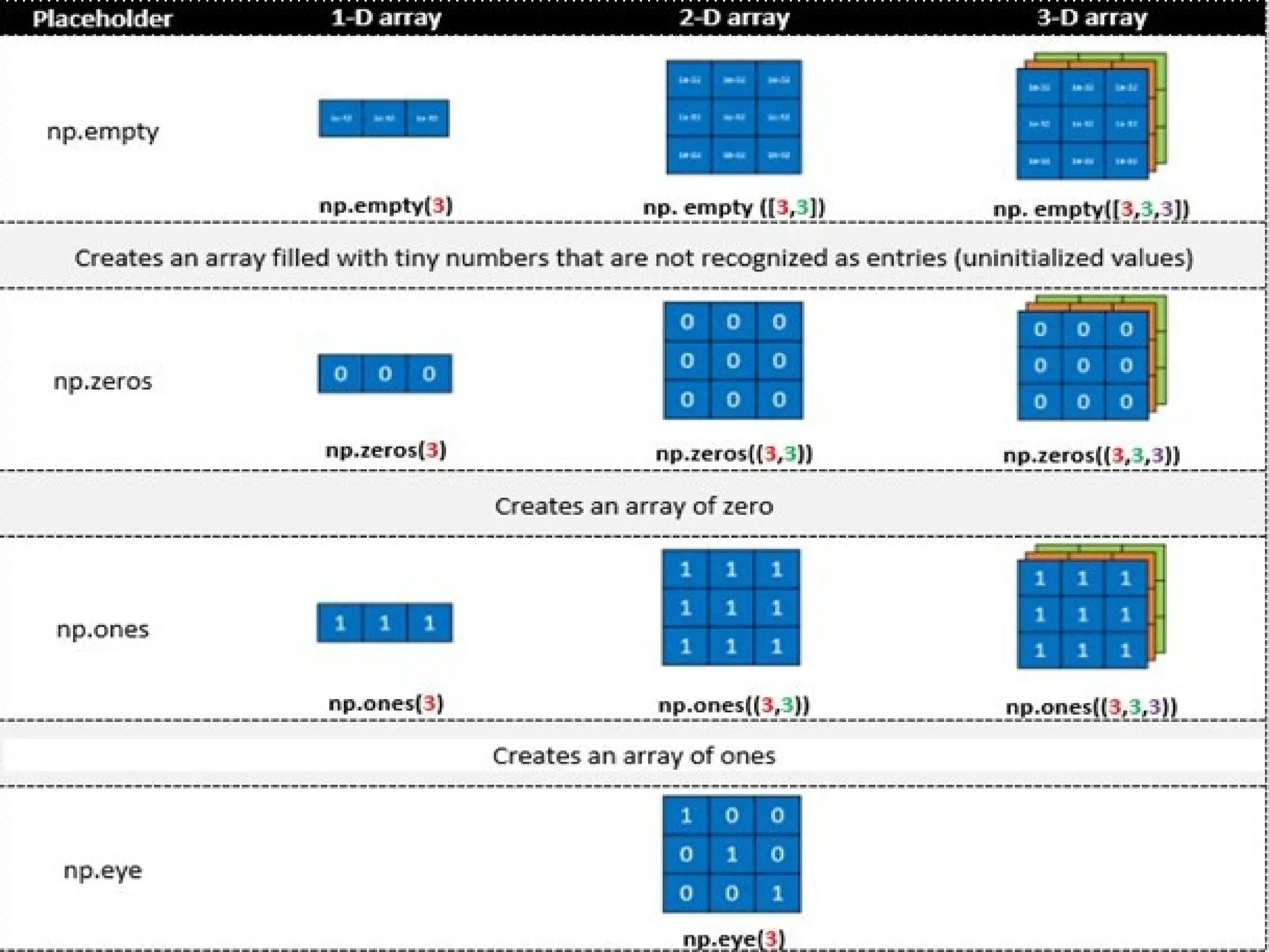
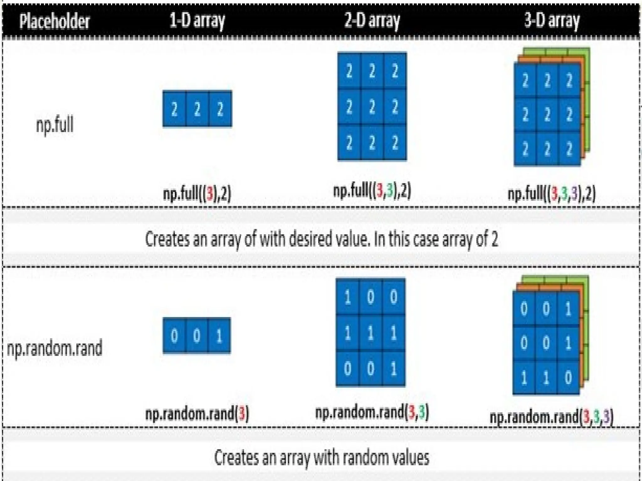
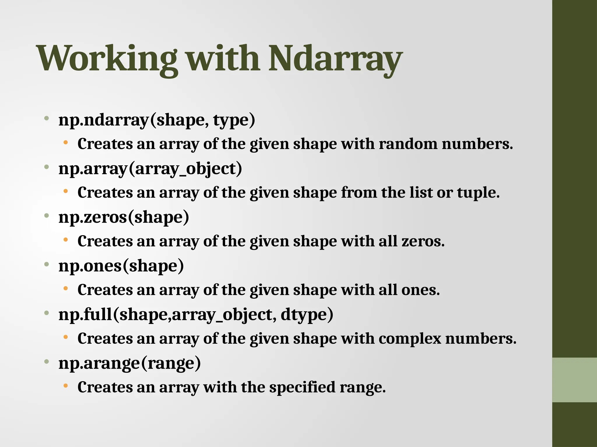
Working with Ndarray •np.ndarray(shape, type) • Creates an array of the given shape with random numbers. • np.array(array_object) • Creates an array of the given shape from the list or tuple. • np.zeros(shape) • Creates an array of the given shape with all zeros. • np.ones(shape) • Creates an array of the given shape with all ones. • np.full(shape,array_object, dtype) • Creates an array of the given shape with complex numbers. • np.arange(range) • Creates an array with the specified range.
87.
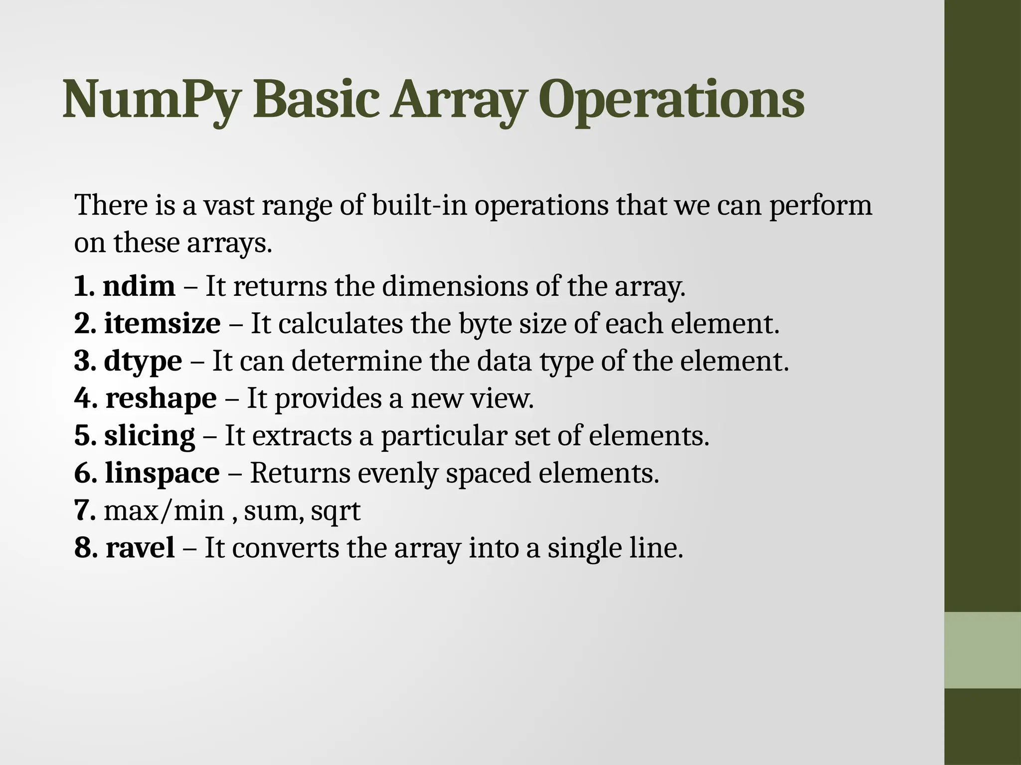
NumPy Basic ArrayOperations There is a vast range of built-in operations that we can perform on these arrays. 1. ndim – It returns the dimensions of the array. 2. itemsize – It calculates the byte size of each element. 3. dtype – It can determine the data type of the element. 4. reshape – It provides a new view. 5. slicing – It extracts a particular set of elements. 6. linspace – Returns evenly spaced elements. 7. max/min , sum, sqrt 8. ravel – It converts the array into a single line.
Copying Arrays Copy fromone array to another • Method 1: Using np.empty_like() function • Method 2: Using np.copy() function • Method 3: Using Assignment Operator
96.
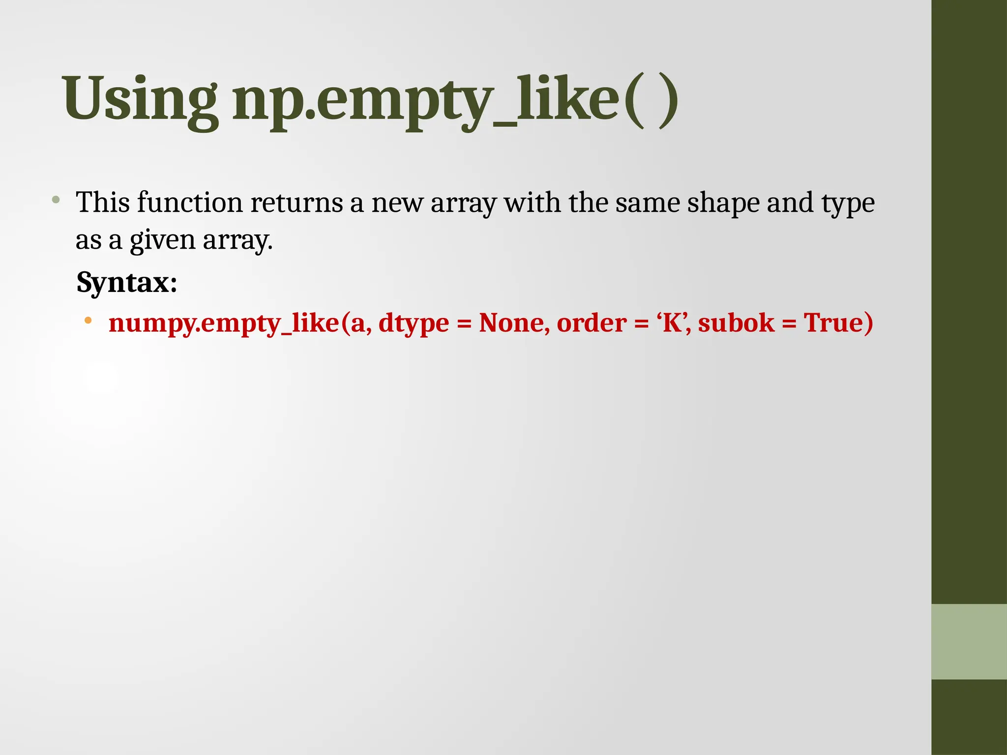
Using np.empty_like( ) •This function returns a new array with the same shape and type as a given array. Syntax: • numpy.empty_like(a, dtype = None, order = ‘K’, subok = True)
97.
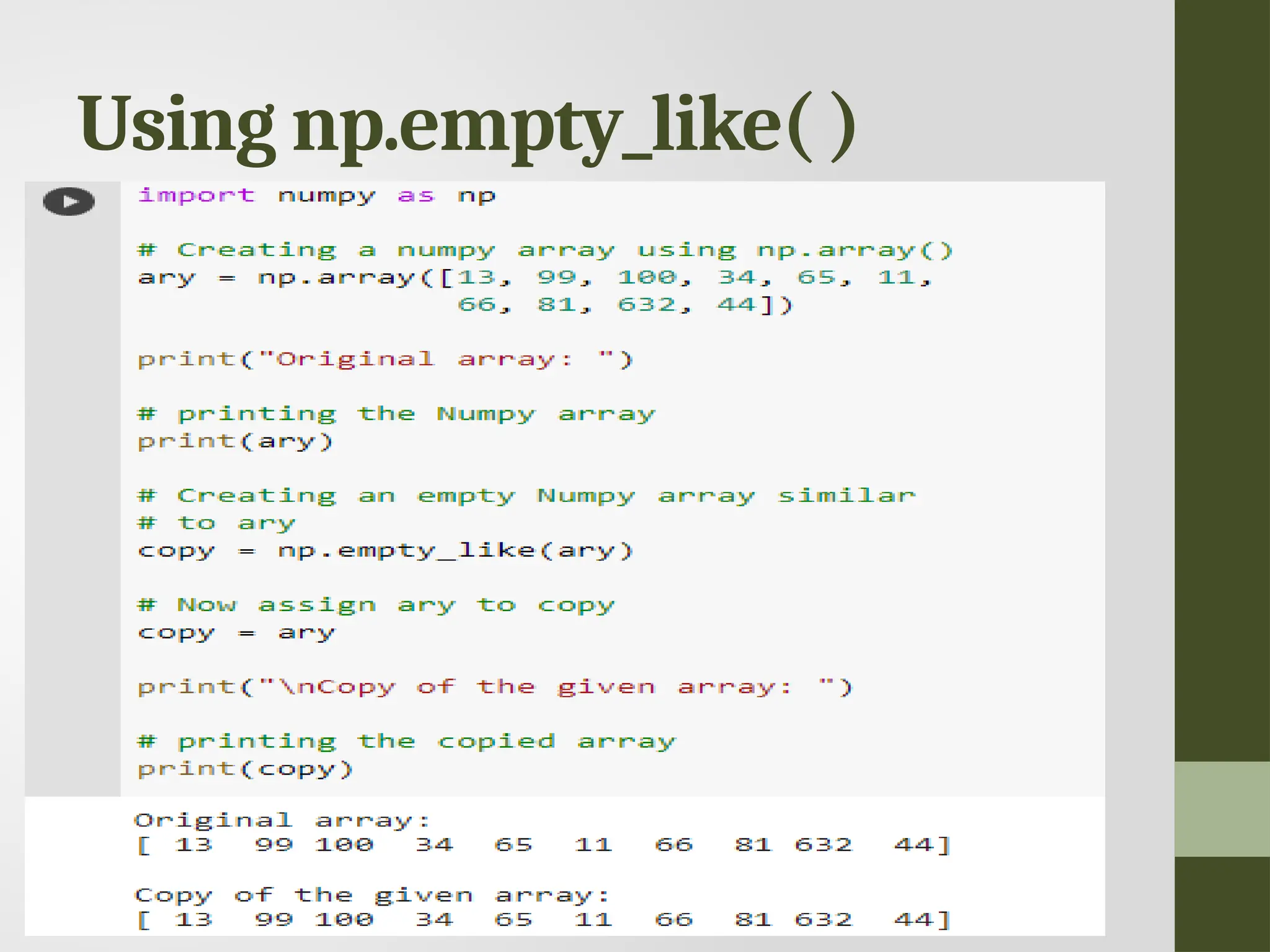
Using np.empty_like( ) •import numpy as np • ary=np.array([13,99,100,34,65,11,66,81,632,44]) • print("Original array: ") • # printing the Numpy array • print(ary) • # Creating an empty Numpy array similar to ary • copy=np.empty_like(ary) • # Now assign ary to copy • copy=ary • print("nCopy of the given array: ") • # printing the copied array • print(copy)
Using np.copy() function •This function returns an array copy of the given object. Syntax : • numpy.copy(a, order='K', subok=False) # importing Numpy package import numpy as np org_array = np.array([1.54, 2.99, 3.42, 4.87, 6.94, 8.21, 7.65, 10.50, 77.5]) print("Original array: ") print(org_array) # Now copying the org_array to copy_array using np.copy() function copy_array = np.copy(org_array) print("nCopied array: ") # printing the copied Numpy array print(copy_array)
100.
Using np.copy() function #importing Numpy package import numpy as np org_array = np.array([1.54, 2.99, 3.42, 4.87, 6.94, 8.21, 7.65, 10.50, 77.5]) print("Original array: ") print(org_array) copy_array = np.copy(org_array) print("nCopied array: ") # printing the copied Numpy array print(copy_array)
101.
Using Assignment Operator importnumpy as np org_array = np.array([[99, 22, 33],[44, 77, 66]]) # Copying org_array to copy_array using Assignment operator copy_array = org_array # modifying org_array org_array[1, 2] = 13 # checking if copy_array has remained the same # printing original array print('Original Array: n', org_array) # printing copied array print('nCopied Array: n', copy_array)
102.
Iterating Arrays • Iteratingmeans going through elements one by one. • As we deal with multi-dimensional arrays in numpy, we can do this using basic for loop of python. • If we iterate on a 1-D array it will go through each element one by one. • Iterate on the elements of the following 1-D array: import numpy as np arr = np.array([1, 2, 3]) for x in arr: print(x) Output: 1 2 3
103.
Iterating Arrays • Iterating2-D Arrays • In a 2-D array it will go through all the rows. • If we iterate on a n-D array it will go through (n-1)th dimension one by one. import numpy as np arr = np.array([[1, 2, 3], [4, 5, 6]]) for x in arr: print(x) Output: [1 2 3] [4 5 6]
104.
Iterating Arrays • Toreturn the actual values, the scalars, we have to iterate the arrays in each dimension. arr = np.array([[1, 2, 3], [4, 5, 6]]) for x in arr: for y in x: print(y) 1 2 3 4 5 6
105.
Iterating Arrays • Iterating3-D Arrays • In a 3-D array it will go through all the 2-D arrays. • import numpy as np arr = np.array([[[1, 2, 3], [4, 5, 6]], [[7, 8, 9], [10, 11, 12]]]) for x in arr: print(x) [[1 2 3] [4 5 6]] [[ 7 8 9] [10 11 12]]
106.
Iterating Arrays • Iterating3-D Arrays • To return the actual values, the scalars, we have to iterate the arrays in each dimension. import numpy as np arr = np.array([[[1, 2, 3], [4, 5, 6]], [[7, 8, 9], [10, 11, 12]]]) for x in arr: for y in x: for z in y: print(z)
107.
Iterating Arrays Usingnditer() • The function nditer() is a helping function that can be used from very basic to very advanced iterations. • Iterating on Each Scalar Element • In basic for loops, iterating through each scalar of an array we need to use n for loops which can be difficult to write for arrays with very high dimensionality. import numpy as np arr = np.array([[[1, 2], [3, 4]], [[5, 6], [7, 8]]]) for x in np.nditer(arr): print(x) 1 2 3 4 5 6 7 8 1 2 3 4 5 6 7 8 1 2 3 4 5 6 7 8
108.
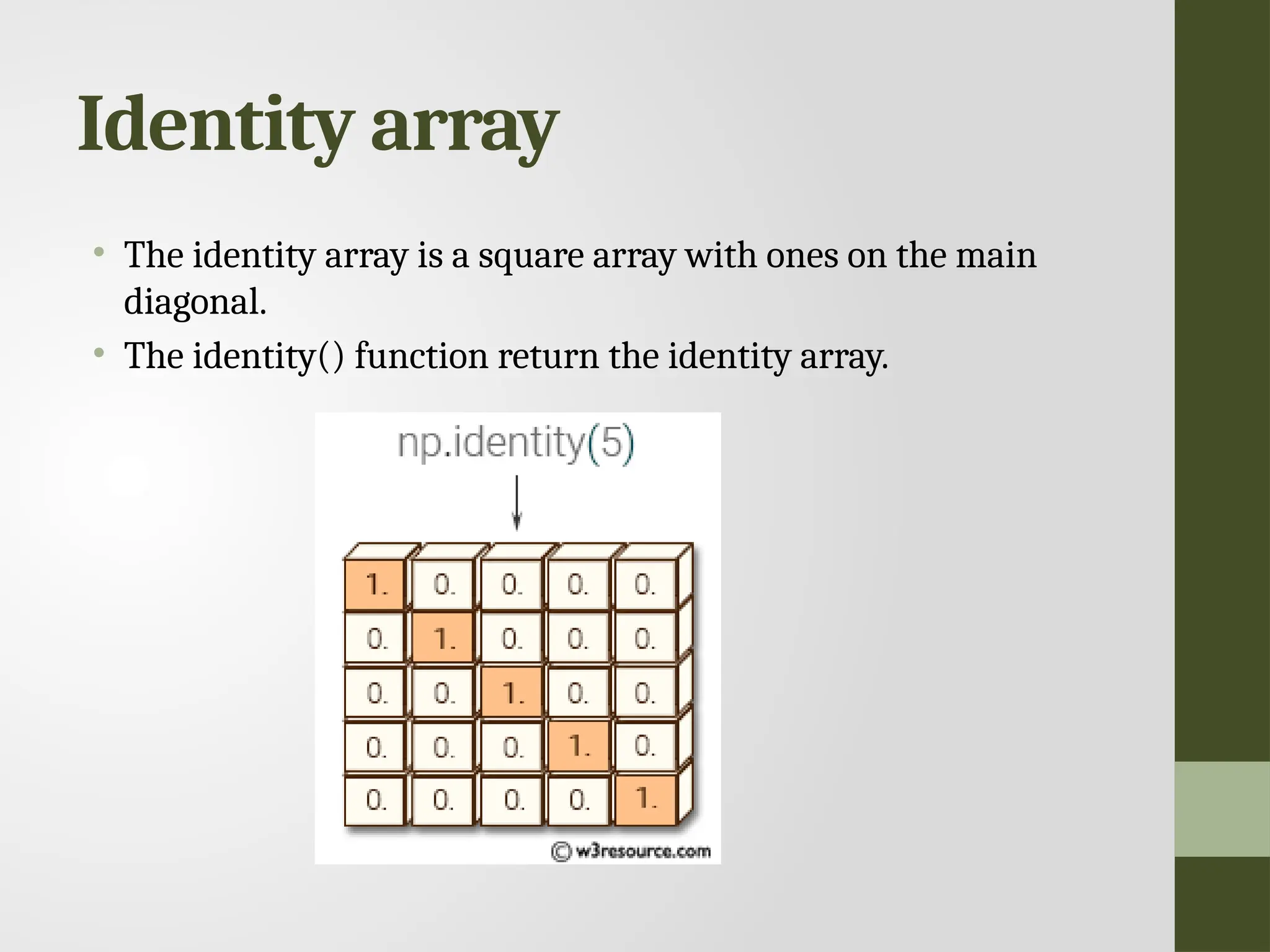
Identity array • Theidentity array is a square array with ones on the main diagonal. • The identity() function return the identity array.
109.
Identity • numpy.identity(n, dtype= None) : Return a identity matrix i.e. a square matrix with ones on the main daignol • Parameters: • n : [int] Dimension n x n of output array • dtype : [optional, float(by Default)] Data type of returned array
110.
Identity array # 2x2matrix with 1's on main diagonal b = np.identity(2, dtype = float) print("Matrix b : n", b) a = np.identity(4) print("nMatrix a : n", a) Output: Matrix b : [[ 1. 0.] [ 0. 1.]] Matrix a : [[ 1. 0. 0. 0.] [ 0. 1. 0. 0.] [ 0. 0. 1. 0.] [ 0. 0. 0. 1.]]
111.
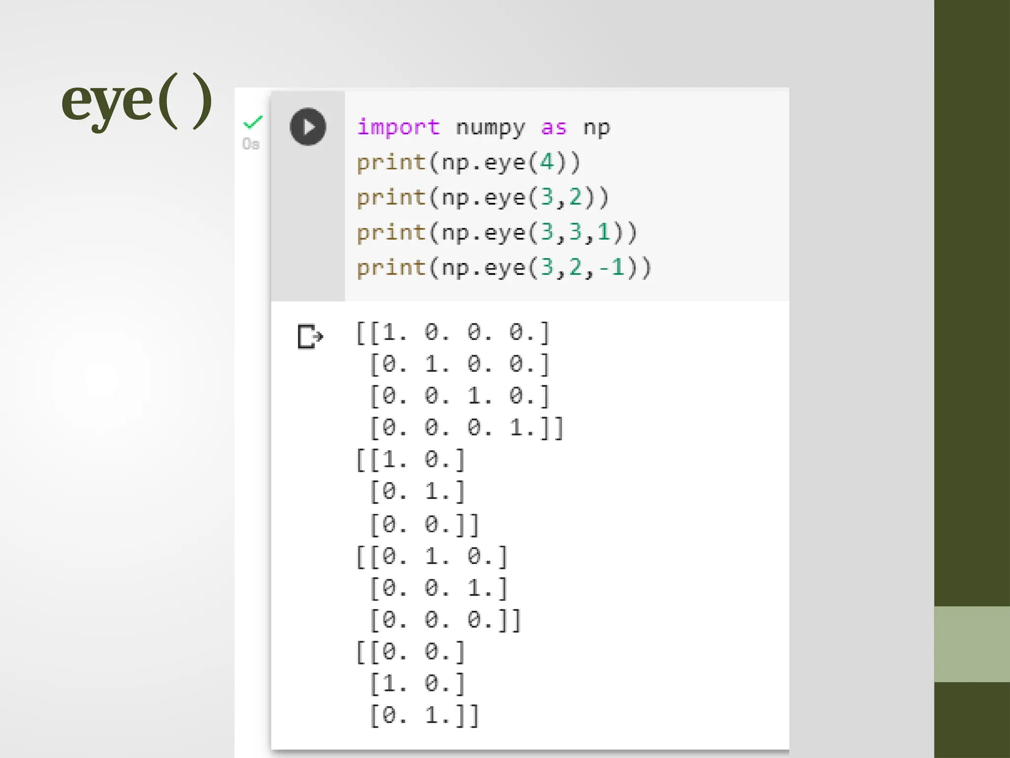
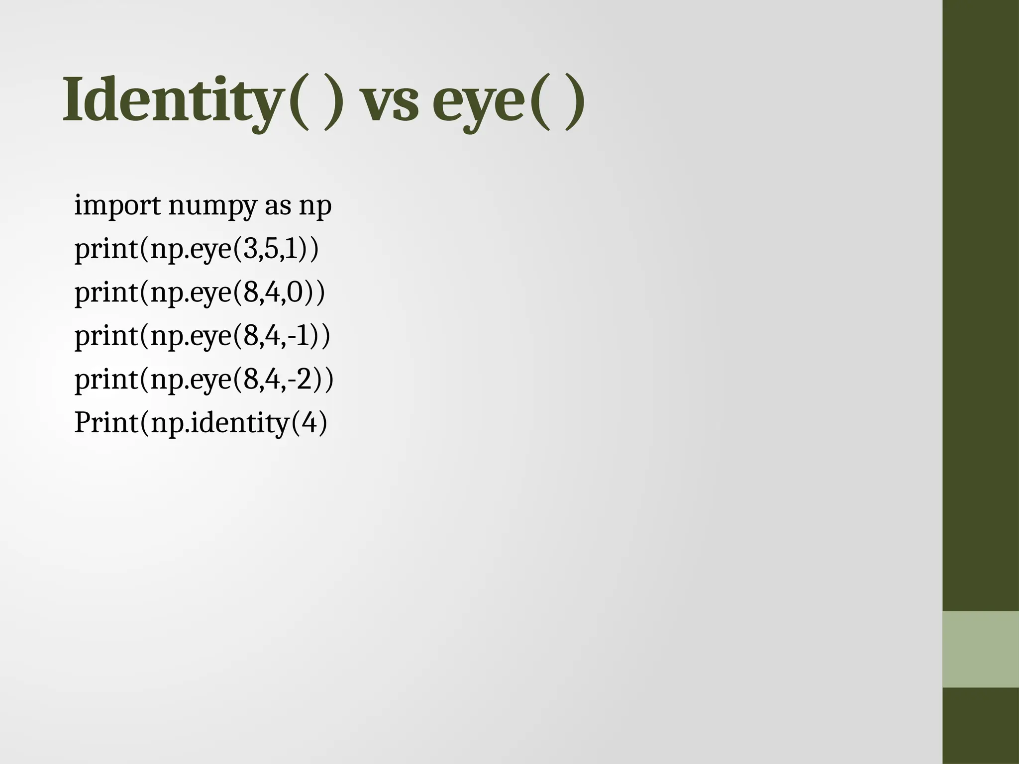
eye( ) • numpy.eye(R,C = None, k = 0, dtype = type <‘float’>) : Return a matrix having 1’s on the diagonal and 0’s elsewhere w.r.t. k. • R : Number of rows C : [optional] Number of columns; By default M = N k : [int, optional, 0 by default] Diagonal we require; k>0 means diagonal above main diagonal or vice versa. dtype : [optional, float(by Default)] Data type of returned array.
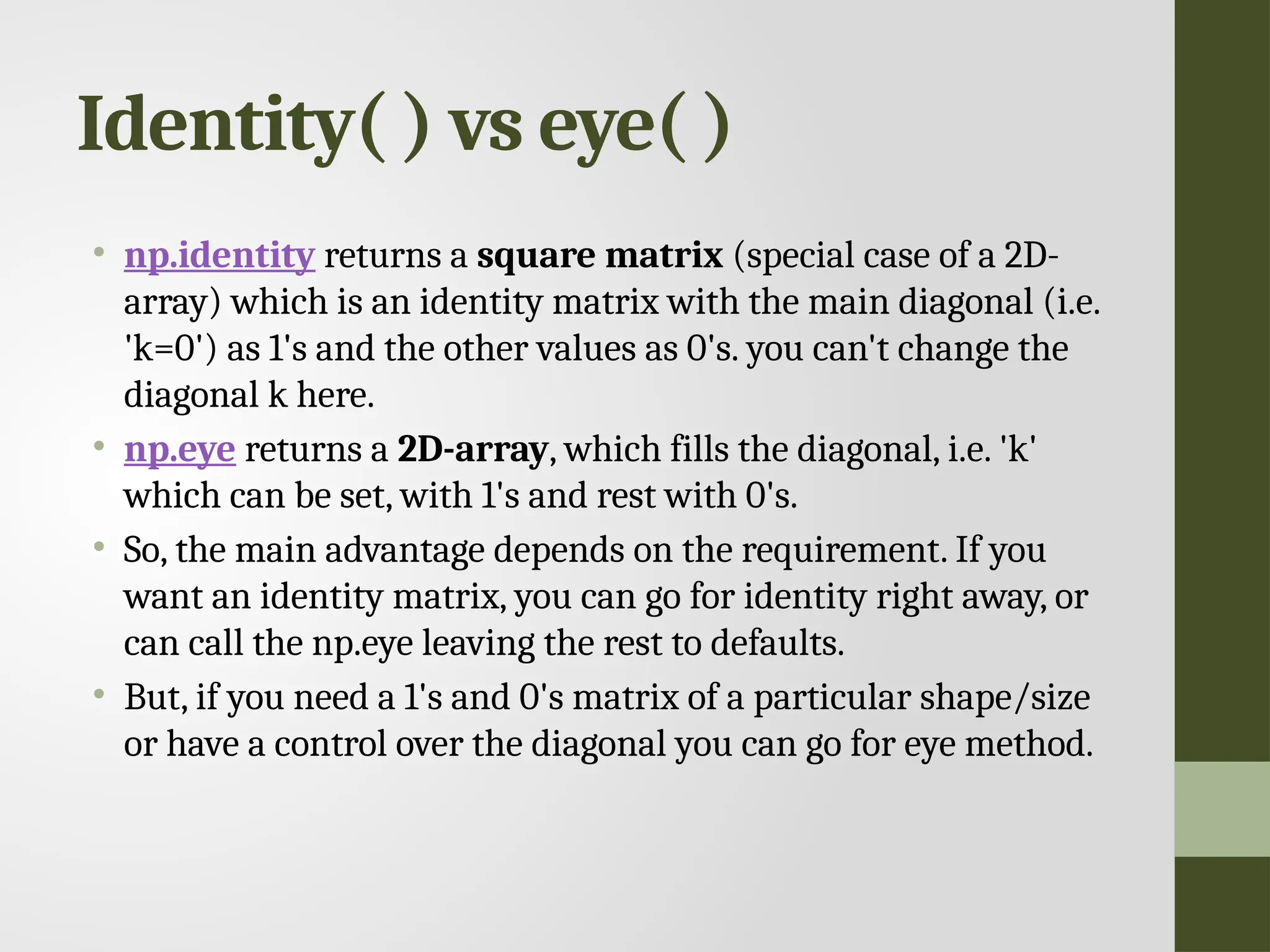
Identity( ) vseye( ) • np.identity returns a square matrix (special case of a 2D- array) which is an identity matrix with the main diagonal (i.e. 'k=0') as 1's and the other values as 0's. you can't change the diagonal k here. • np.eye returns a 2D-array, which fills the diagonal, i.e. 'k' which can be set, with 1's and rest with 0's. • So, the main advantage depends on the requirement. If you want an identity matrix, you can go for identity right away, or can call the np.eye leaving the rest to defaults. • But, if you need a 1's and 0's matrix of a particular shape/size or have a control over the diagonal you can go for eye method.
Reshaping arrays • Reshapingmeans changing the shape of an array. • The shape of an array is the number of elements in each dimension. • By reshaping we can add or remove dimensions or change number of elements in each dimension.
Reshape From 1-Dto 3-D • The outermost dimension will have 2 arrays that contains 3 arrays, each with 2 elements • import numpy as np arr = np.array([1, 2, 3, 4, 5, 6, 7, 8, 9, 10, 11, 12]) newarr = arr.reshape(2, 3, 2) print(newarr) Output: [[[ 1 2] [ 3 4] [ 5 6]] [[ 7 8] [ 9 10] [11 12]]]
119.
Can we Reshapeinto any Shape? • Yes, as long as the elements required for reshaping are equal in both shapes. • We can reshape an 8 elements 1D array into 4 elements in 2 rows 2D array but we cannot reshape it into a 3 elements 3 rows 2D array as that would require 3x3 = 9 elements. import numpy as np arr = np.array([1, 2, 3, 4, 5, 6, 7, 8]) newarr = arr.reshape(3, 3) print(newarr) • Traceback (most recent call last): File "demo_numpy_array_reshape_error.py", line 5, in <module> ValueError: cannot reshape array of size 8 into shape (3,3)
120.
Flattening the arrays •Flattening array means converting a multidimensional array into a 1D array. • import numpy as np arr = np.array([[1, 2, 3], [4, 5, 6]]) newarr = arr.reshape(-1) print(newarr) • Output: [1 2 3 4 5 6] • There are a lot of functions for changing the shapes of arrays in numpy flatten, ravel and also for rearranging the elements rot90, flip, fliplr, flipud etc. These fall under Intermediate to Advanced section of numpy.
Pandas • Pandas isa popular open-source data manipulation and analysis library for Python. • It provides easy-to-use data structures like DataFrame and Series, which are designed to make working with structured data fast, easy, and expressive. • Pandas are widely used in data science, machine learning, and data analysis for tasks such as data cleaning, transformation, and exploration.
123.
Series • A PandasSeries is a one-dimensional array-like object that can hold data of any type (integer, float, string, etc.). • It is labelled, meaning each element has a unique identifier called an index. • Series is defined as a column in a spreadsheet or a single column of a database table. • Series are a fundamental data structure in Pandas and are commonly used for data manipulation and analysis tasks. • They can be created from lists, arrays, dictionaries, and existing Series objects. • Series are also a building block for the more complex Pandas DataFrame, which is a two-dimensional table-like structure consisting of multiple Series objects.
124.
Series import pandas aspd # Initializing a Series from a list data = [1, 2, 3, 4, 5] series_from_list = pd.Series(data) print(series_from_list) # Initializing a Series from a dictionary data = {'a': 1, 'b': 2, 'c': 3} series_from_dict = pd.Series(data) print(series_from_dict) # Initializing a Series with custom index data = [1, 2, 3, 4, 5] index = ['a', 'b', 'c', 'd', 'e'] series_custom_index = pd.Series(data, index=index) print(series_custom_index) Output 0 1 1 2 2 3 3 4 4 5 dtype: int64 a 1 b 2 c 3 dtype: int64 a 1 b 2 c 3 d 4 e 5 dtype: int64
125.
Series - Indexing •Each element in a Series has a corresponding index, which can be used to access or manipulate the data. print(series_from_list[0]) print(series_from_dict['b’]) Output 1 2
126.
Series – Vectorized Operations •Series supports vectorized operations, allowing you to perform arithmetic operations on the entire series efficiently. series_a = pd.Series([1, 2, 3]) series_b = pd.Series([4, 5, 6]) sum_series = series_a + series_b print(sum_series) Output 0 5 1 7 2 9 dtype: int64
127.
Series – Alignment •When performing operations between two Series objects, Pandas automatically aligns the data based on the index labels. series_a = pd.Series([1, 2, 3], index=['a', 'b', 'c']) series_b = pd.Series([4, 5, 6], index=['b', 'c', 'd']) sum_series = series_a + series_b print(sum_series) Output a NaN b 6.0 c 8.0 d NaN dtype: float64
128.
Series – NaNHandling • Missing values, represented by NaN (Not a Number), can be handled gracefully in Series operations. series_a = pd.Series([1, 2, 3], index=['a', 'b', 'c']) series_b = pd.Series([4, 5], index=['b', 'c']) sum_series = series_a + series_b print(sum_series) Output a NaN b 6.0 c 8.0 dtype: float64
129.
DataFrame • A PandasDataFrame is a two-dimensional, tabular data structure with rows and columns. • It is similar to a spreadsheet or a table in a relational database. • The DataFrame has three main components: • data, which is stored in rows and columns; • rows, which are labeled by an index; • columns, which are labeled and contain the actual data.
130.
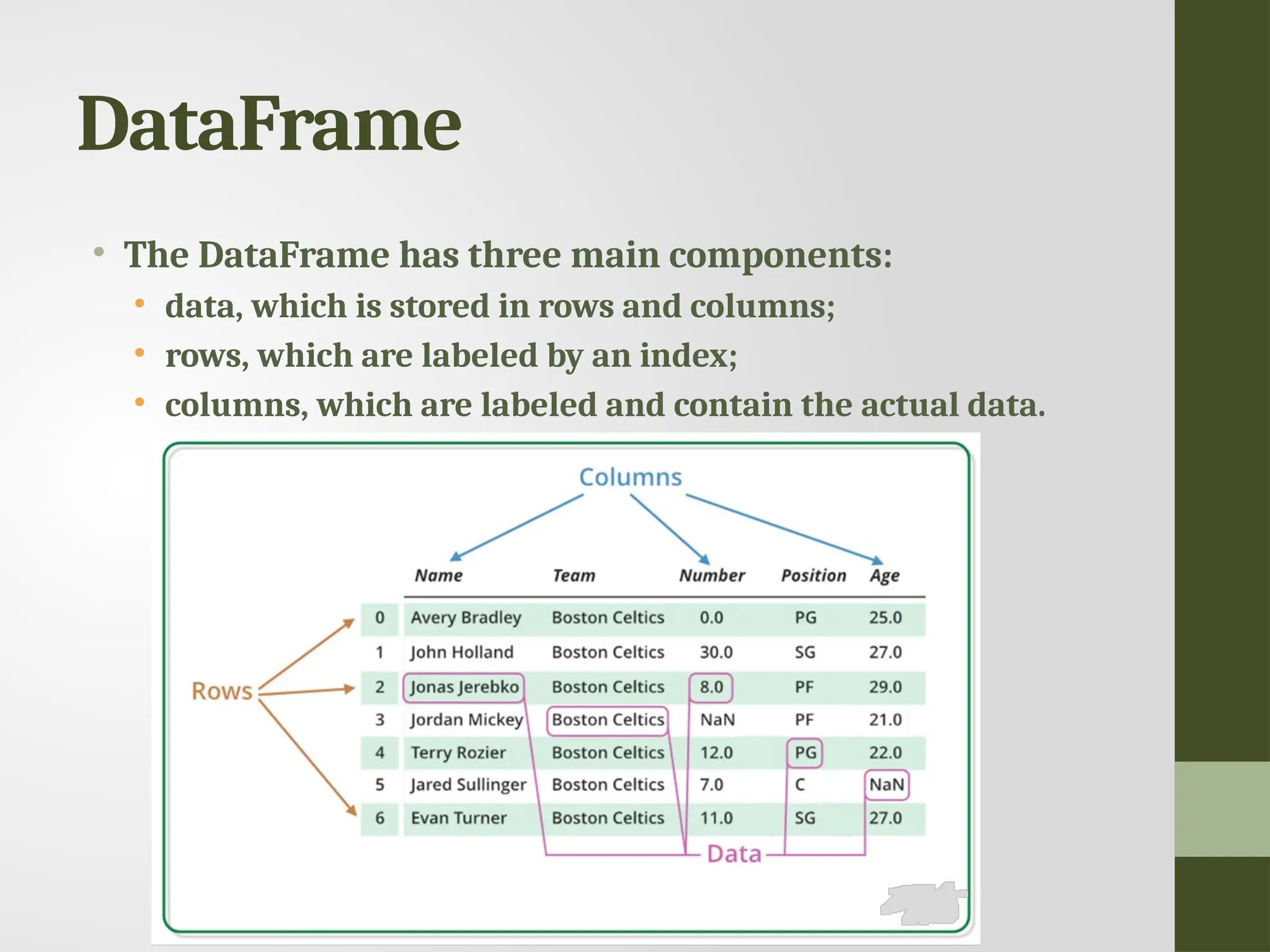
DataFrame • The DataFramehas three main components: • data, which is stored in rows and columns; • rows, which are labeled by an index; • columns, which are labeled and contain the actual data.
131.
DataFrames import pandas aspd # Initializing a DataFrame from a dictionary data = {'Name': ['John', 'Alice', 'Bob'], 'Age': [25, 30, 35], 'City': ['New York', 'Los Angeles', 'Chicago']} df = pd.DataFrame(data) print(df) # Initializing a DataFrame from a list of lists data = [['John', 25, 'New York'], ['Alice', 30, 'Los Angeles'], ['Bob', 35, 'Chicago']] columns = ['Name', 'Age', 'City'] df = pd.DataFrame(data, columns=columns) print(df) Name Age City 0 John 25 New York 1 Alice 30 Los Angeles 2 Bob 35 Chicago Name Age City 0 John 25 New York 1 Alice 30 Los Angeles 2 Bob 35 Chicago
132.
DataFrames - Indexing •DataFrame provides flexible indexing options, allowing access to rows, columns, or individual elements based on labels or integer positions. # Accessing a column print(df['Name']) # Accessing a row by label print(df.loc[0]) # Accessing a row by integer position print(df.iloc[0]) # Accessing an individual element print(df.at[0, 'Name']) 0 John 1 Alice 2 Bob Name: Name, dtype: object Name John Age 25 City New York Name: 0, dtype: object Name John Age 25 City New York Name: 0, dtype: object John
133.
DataFrame – Column Operations •Columns in a DataFrame are Series objects, enabling various operations such as arithmetic operations, filtering, and sorting. # Adding a new column df['Salary'] = [50000, 60000, 70000] # Filtering rows based on a condition high_salary_employees = df[df['Salary'] > 60000] print(high_salary_employees) # Sorting DataFrame by a column sorted_df = df.sort_values(by='Age', ascending=False) print(sorted_df)
134.
DataFrames – Column Operations •Columns in a DataFrame are Series objects, enabling various operations such as arithmetic operations, filtering, and sorting. # Adding a new column df['Salary'] = [50000, 60000, 70000] # Filtering rows based on a condition high_salary_employees = df[df['Salary'] > 60000] print(high_salary_employees) # Sorting DataFrame by a column sorted_df = df.sort_values(by='Age', ascending=False) print(sorted_df) Name Age City Salary 2 Bob 35 Chicago 70000 Name Age City Salary 2 Bob 35 Chicago 70000 1 Alice 30 Los Angeles 60000 0 John 25 New York 50000
135.
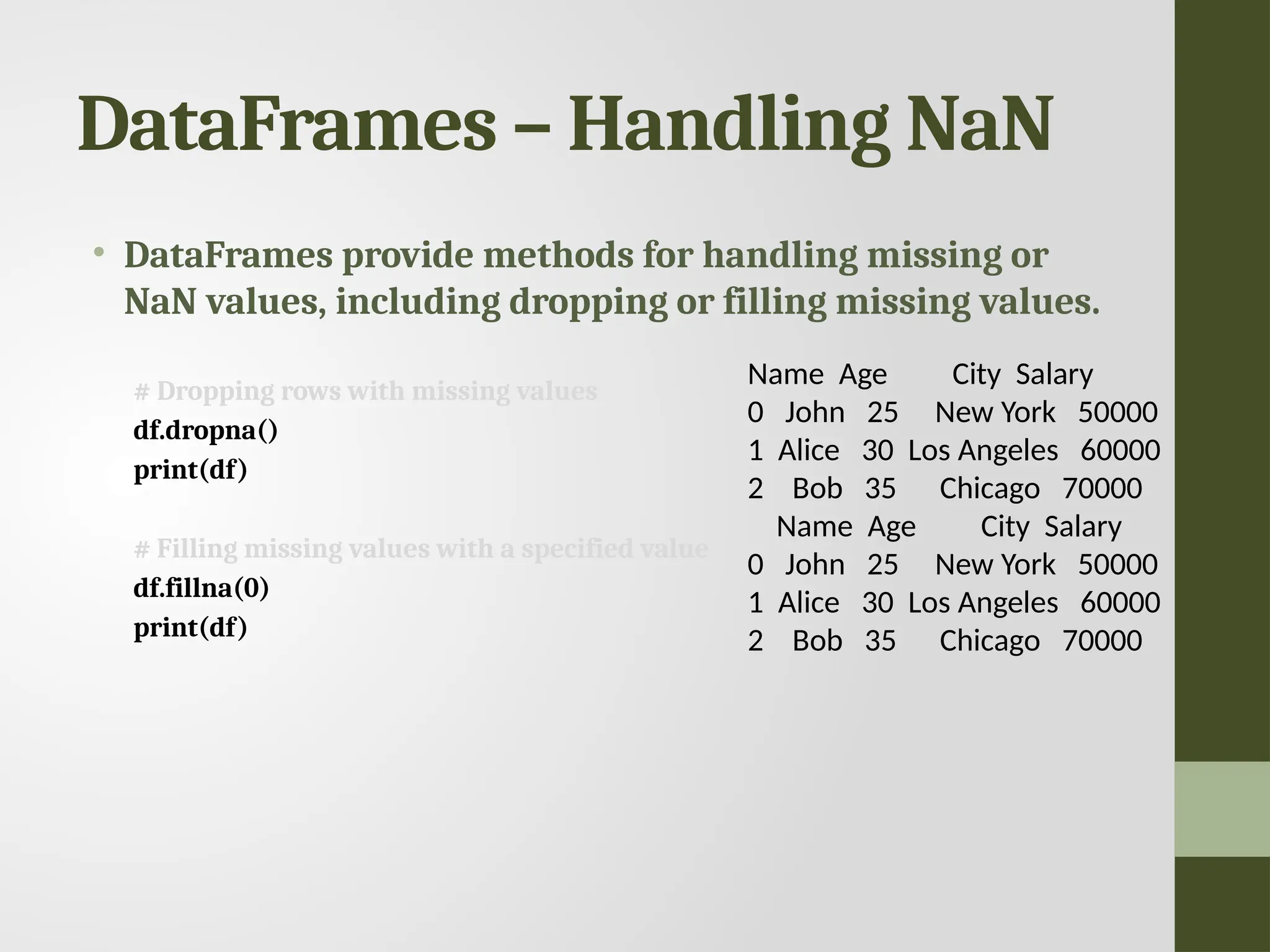
DataFrames – HandlingNaN • DataFrames provide methods for handling missing or NaN values, including dropping or filling missing values. # Dropping rows with missing values df.dropna() print(df) # Filling missing values with a specified value df.fillna(0) print(df) Name Age City Salary 0 John 25 New York 50000 1 Alice 30 Los Angeles 60000 2 Bob 35 Chicago 70000 Name Age City Salary 0 John 25 New York 50000 1 Alice 30 Los Angeles 60000 2 Bob 35 Chicago 70000
136.
DataFrames – Groupingand Aggregation • DataFrames support group-by operations for summarizing data and applying aggregation functions. # Grouping by a column and calculating mean avg_age_by_city = df.groupby('City')['Age'].mean() print(avg_age_by_city) City Chicago 35.0 Los Angeles 30.0 New York 25.0 Name: Age, dtype: float64
137.
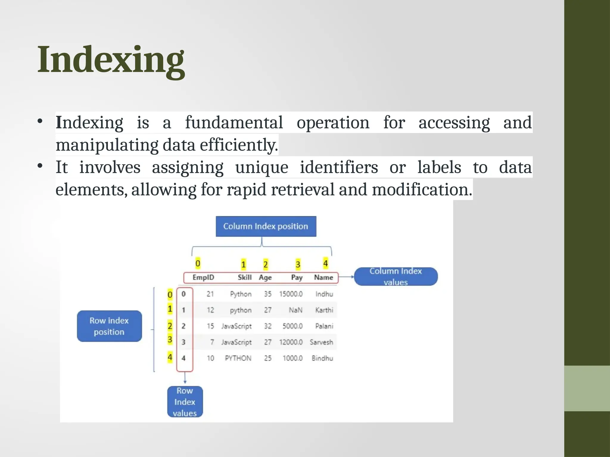
Indexing • Indexing isa fundamental operation for accessing and manipulating data efficiently. • It involves assigning unique identifiers or labels to data elements, allowing for rapid retrieval and modification.
138.
Indexing - Features •Immutability: Once created, an index cannot be modified. • Alignment: Index objects are used to align data structures like Series and DataFrames. • Flexibility: Pandas offers various index types, including integer-based, datetime, and custom indices.
139.
Index - Creation importpandas as pd data = {'Name': ['Alice', 'Bob', 'Charlie'], 'Age': [25, 30, 35]} df = pd.DataFrame(data, index=['A', 'B', 'C'])
140.
Re-index • Reindexing isthe process of creating a new DataFrame or Series with a different index. • The reindex() method is used for this purpose. import pandas as pd data = {'Name': ['Alice', 'Bob', 'Charlie’], 'Age': [25, 30, 35]} df = pd.DataFrame(data, index=['A', 'B', 'C’]) # Create a new index new_index = ['A', 'B', 'D', 'E'] # Reindex the DataFrame df_reindexed = df.reindex(new_index) df_reindexed
141.
Drop Entry • Droppingentries in data science refers to removing specific rows or columns from a dataset. • This is a common operation in data cleaning and preprocessing to handle missing values, outliers, or irrelevant information.
142.
Drop Entry data ={'Name': ['Alice', 'Bob', 'Charlie'], 'Age': [25, 30, 35]} df = pd.DataFrame(data) df # Drop column newdf = df.drop("Age", axis='columns') newdf
143.
Selecting Entries –Selecting by Position import pandas as pd data = {'Name': ['Alice', 'Bob', 'Charlie'], 'Age': [25, 30, 35], 'City': ['New York', 'Los Angeles’, 'Chicago']} df = pd.DataFrame(data) # Select the second row df.iloc[1] Selecting data by Position Created DataFrame
144.
Selecting Entries –Selecting by Condition import pandas as pd data = {'Name': ['Alice', 'Bob', 'Charlie'], 'Age': [25, 30, 35], 'City': ['New York', 'Los Angeles’, 'Chicago']} df = pd.DataFrame(data) # Select rows where Age is greater than 30 df[df['Age'] > 30] Selecting data by Condition Created DataFrame
145.
Data Alignment • Dataalignment is intrinsic, which means that it's inherent to the operations you perform. • Align data in them by their labels and not by their position • align( ) function is used to align • Used to align two data objects with each other according to their labels. • Used on both Series and DataFrame objects • Returns a new object of the same type with labels compared and aligned.
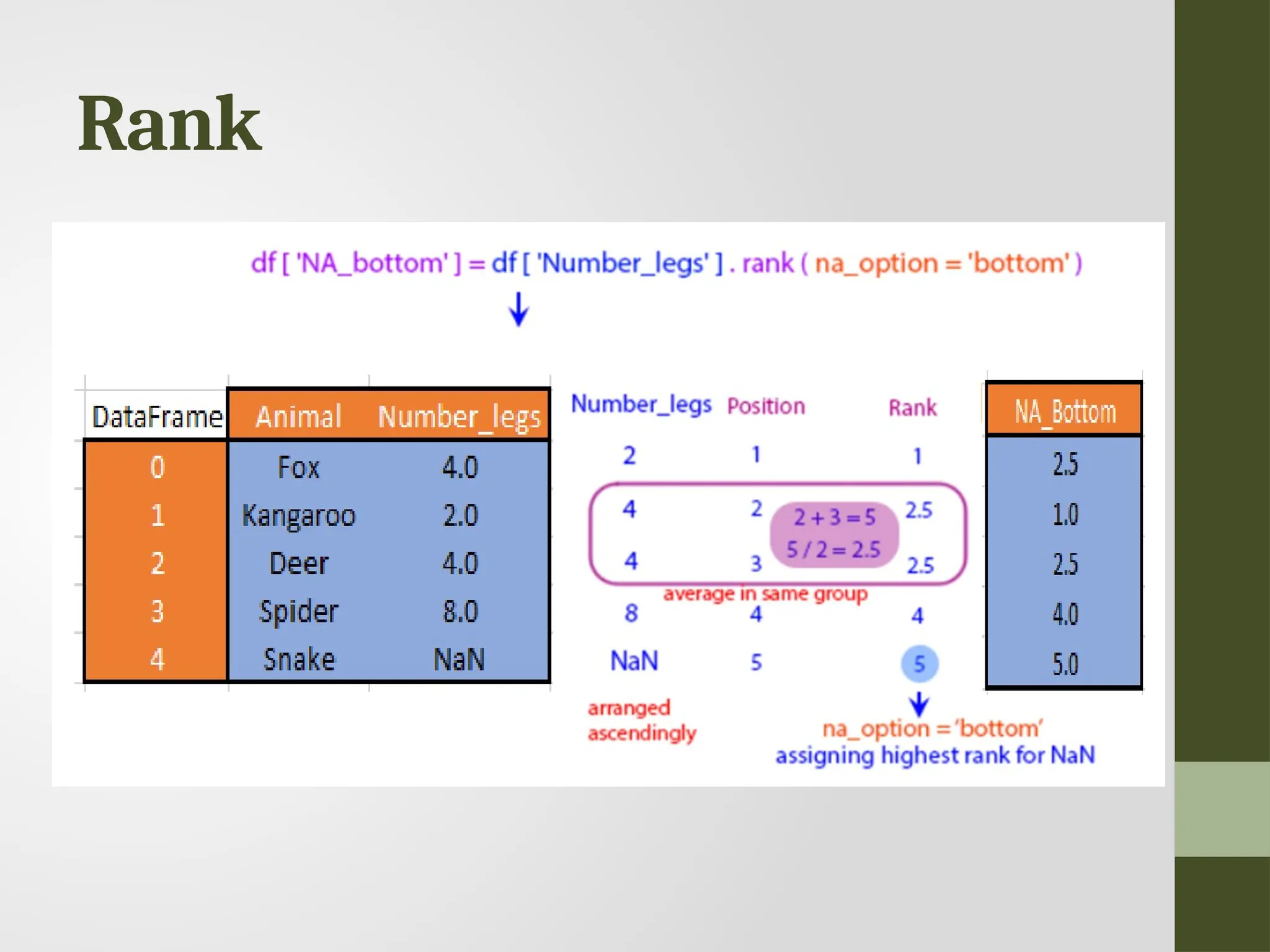
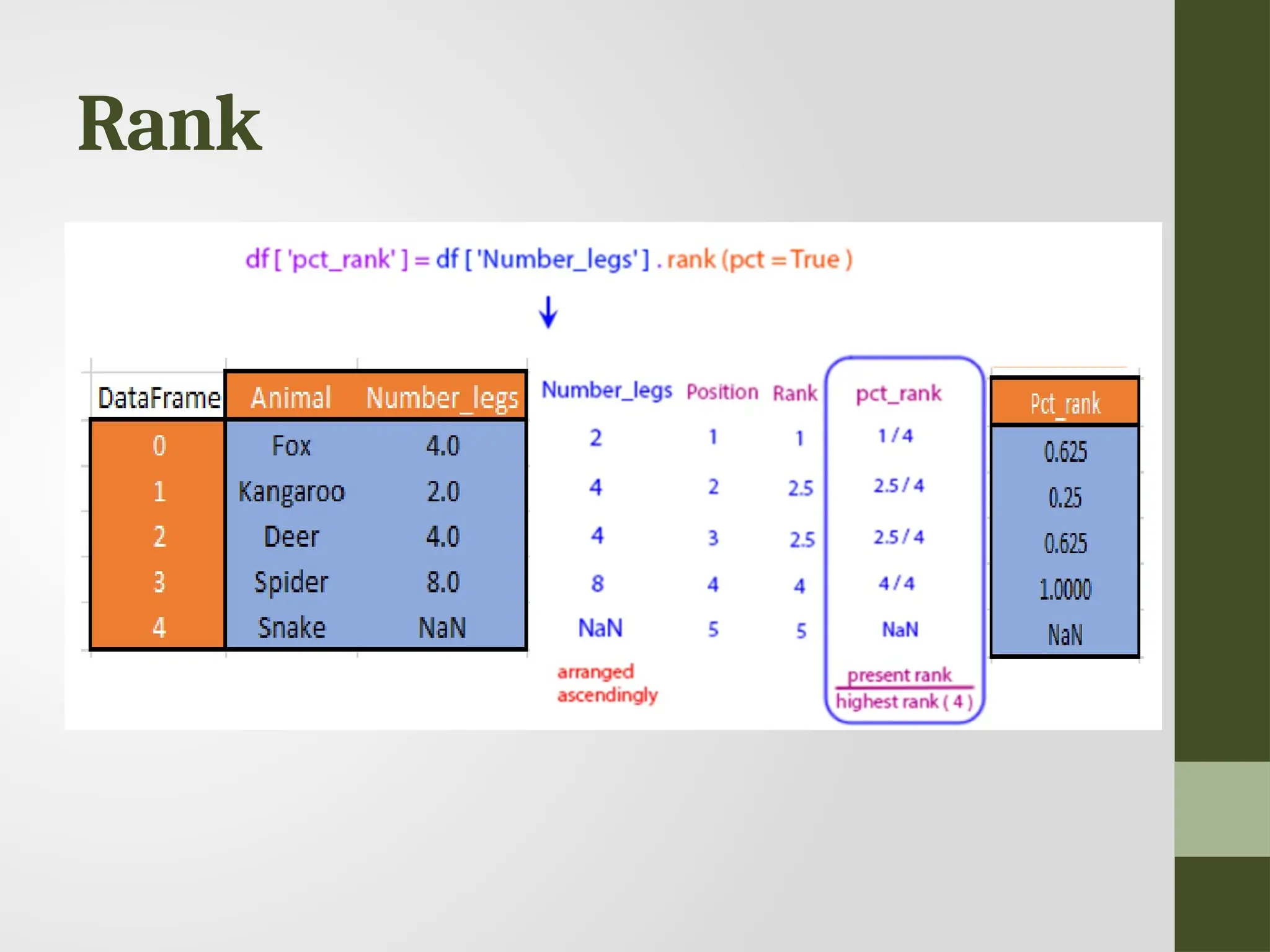
Rank • Ranking isassigning ranks or positions to data elements based on their values. • Rank is returned based on position after sorting. • Used when analyzing data with repetitive values or when you need to identify the top or bottom entries.
Sort • Sort bythe values along the axis • Sort a pandas DataFrame by the values of one or more columns • Use the ascending parameter to change the sort order • Sort a DataFrame by its index using .sort_index() • Organize missing data while sorting values • Sort a DataFrame in place using inplace set to True
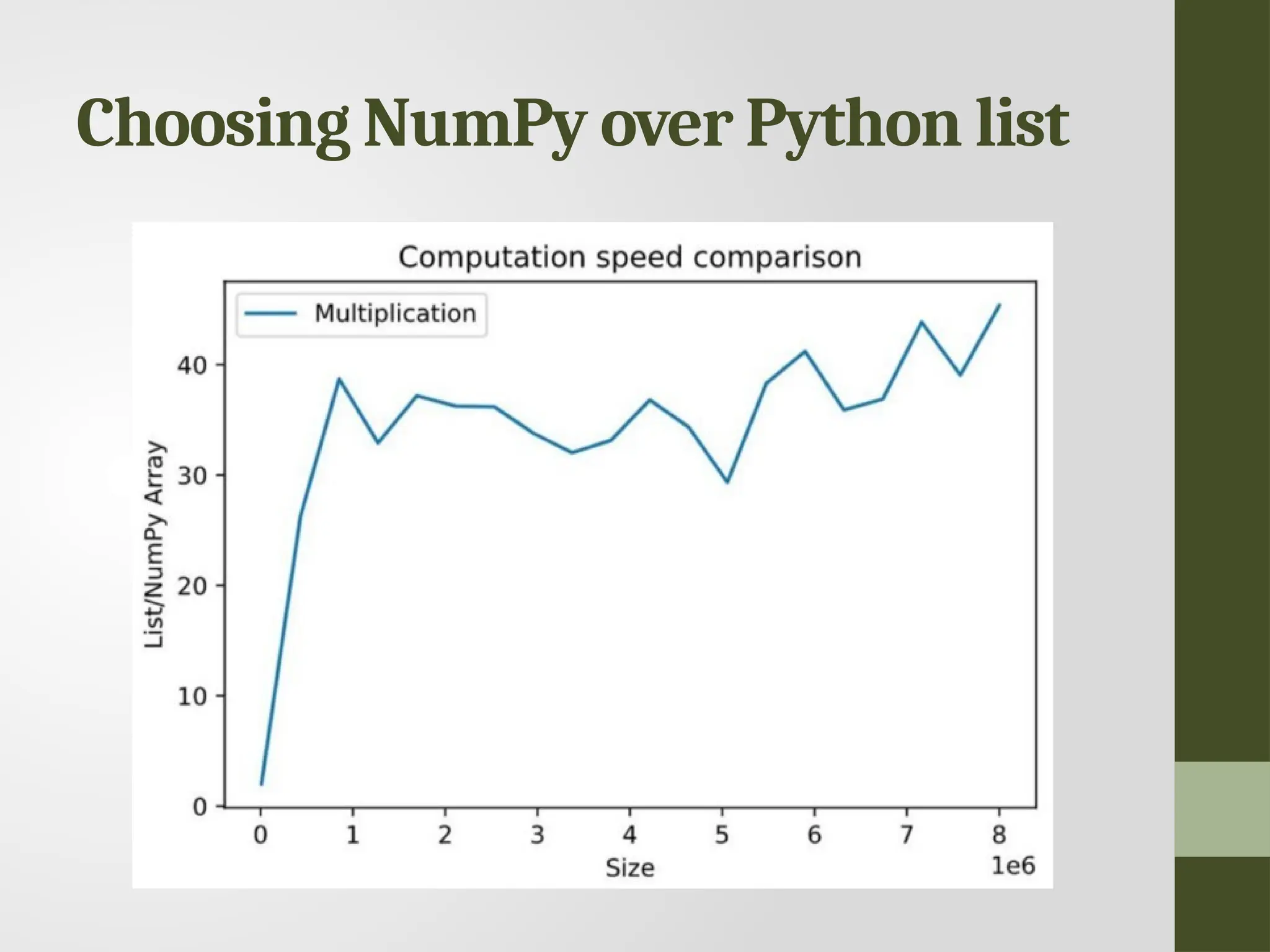
#69 NumPy offers low memory consumption, high speed, and massive lists of functionalities compared to traditional lists. NumPy can divide a task and process them parallelly, which makes them highly efficient. The figure shows the ratio of computation time of list/NumPy array vs. size. Computation time for the multiplication of two Python lists drastically increases with list size compared to NumPy arrays. Multiplication of two NumPy arrays with 100,000 elements is ~40 times faster than the Python list with the same number of elements. Hence, NumPy is the better solution for arrays with a large number of elements.


![Array • Similar to the indexing of lists • Zero-based indexing • [10, 9, 99, 71, 90 ]](https://image.slidesharecdn.com/uniti-datascience-250227192810-b6dbd39e/75/Data-Science-presentation-for-explanation-of-numpy-and-pandas-71-2048.jpg)

![1. Using the NumPy functions a. Creating one-dimensional array in NumPy import numpy as np array=np.arange(20) array Output: array([ 0, 1, 2, 3, 4, 5, 6, 7, 8, 9, 10, 11,12, 13, 14, 15, 16, 17, 18, 19])](https://image.slidesharecdn.com/uniti-datascience-250227192810-b6dbd39e/75/Data-Science-presentation-for-explanation-of-numpy-and-pandas-75-2048.jpg)
![1. Using the NumPy functions a. check the dimensions by using array.shape. (20, ) Output: array([ 0 1 2 3 4 5 6 7 8 9 10 1112 13 14,15, 16, 17, 18, 19])](https://image.slidesharecdn.com/uniti-datascience-250227192810-b6dbd39e/75/Data-Science-presentation-for-explanation-of-numpy-and-pandas-76-2048.jpg)
![1. Using the NumPy functions b. Creating two-dimensional arrays in NumPy array=np.arange(20).reshape(4,5) Output: array([[ 0, 1, 2, 3, 4], [ 5, 6, 7, 8, 9], [10, 11, 12, 13, 14] [15, 16, 17, 18, 19]])](https://image.slidesharecdn.com/uniti-datascience-250227192810-b6dbd39e/75/Data-Science-presentation-for-explanation-of-numpy-and-pandas-77-2048.jpg)
![1. Using the NumPy functions c. Using other NumPy functions np.zeros((2,4)) np.ones((3,6)) np.full((2,2), 3) Output: array([[0., 0., 0., 0.], [0., 0., 0., 0.]]) array([[1., 1., 1., 1., 1., 1.], [1., 1., 1., 1., 1., 1.], [1., 1., 1., 1., 1., 1.]])](https://image.slidesharecdn.com/uniti-datascience-250227192810-b6dbd39e/75/Data-Science-presentation-for-explanation-of-numpy-and-pandas-78-2048.jpg)
![1. Using the NumPy functions c. Using other NumPy functions import numpy as np a=np.zeros((2,4)) b=np.ones((3,6)) c=np.empty((2,3)) d=np.full((2,2), 3) e= np.eye(3,3) f=np.linspace(0, 10, num=4) print(a) print(b) print(c) print(d) [[0. 0. 0. 0.] [0. 0. 0. 0.]] [[1. 1. 1. 1. 1. 1.] [1. 1. 1. 1. 1. 1.] [1. 1. 1. 1. 1. 1.]] [[1.14137702e-316 0.00000000e+000 6.91583610e-310] [6.91583609e-310 6.91583601e-310 6.91583601e-310]] [[3 3] [3 3]] [[1. 0. 0.] [0. 1. 0.] [0. 0. 1.]] [ 0. 3.33333333 6.66666667 10. ]](https://image.slidesharecdn.com/uniti-datascience-250227192810-b6dbd39e/75/Data-Science-presentation-for-explanation-of-numpy-and-pandas-81-2048.jpg)
![2.ConversionfromPythonstructurelikelists import numpy as np array=np.array([4,5,6]) print(array) list=[4,5,6] print(list) [4 5 6] [4, 5, 6]](https://image.slidesharecdn.com/uniti-datascience-250227192810-b6dbd39e/75/Data-Science-presentation-for-explanation-of-numpy-and-pandas-85-2048.jpg)
![Checking Array Dimensions in NumPy import numpy as np a = np.array(10) b = np.array([1,1,1,1]) c = np.array([[1, 1, 1], [2,2,2]]) d = np.array([[[1, 1, 1], [2, 2, 2]], [[3, 3, 3], [4, 4, 4]]]) print(a.ndim) #0 print(b.ndim) #1 print(c.ndim) #2 print(d.ndim) #3](https://image.slidesharecdn.com/uniti-datascience-250227192810-b6dbd39e/75/Data-Science-presentation-for-explanation-of-numpy-and-pandas-89-2048.jpg)
![Higher Dimensional Arrays in NumPy import numpy as np arr = np.array([1, 1, 1, 1, 1], ndmin=10) print(arr) print('number of dimensions :', arr.ndim) [[[[[[[[[[1 1 1 1 1]]]]]]]]]] number of dimensions : 10](https://image.slidesharecdn.com/uniti-datascience-250227192810-b6dbd39e/75/Data-Science-presentation-for-explanation-of-numpy-and-pandas-90-2048.jpg)
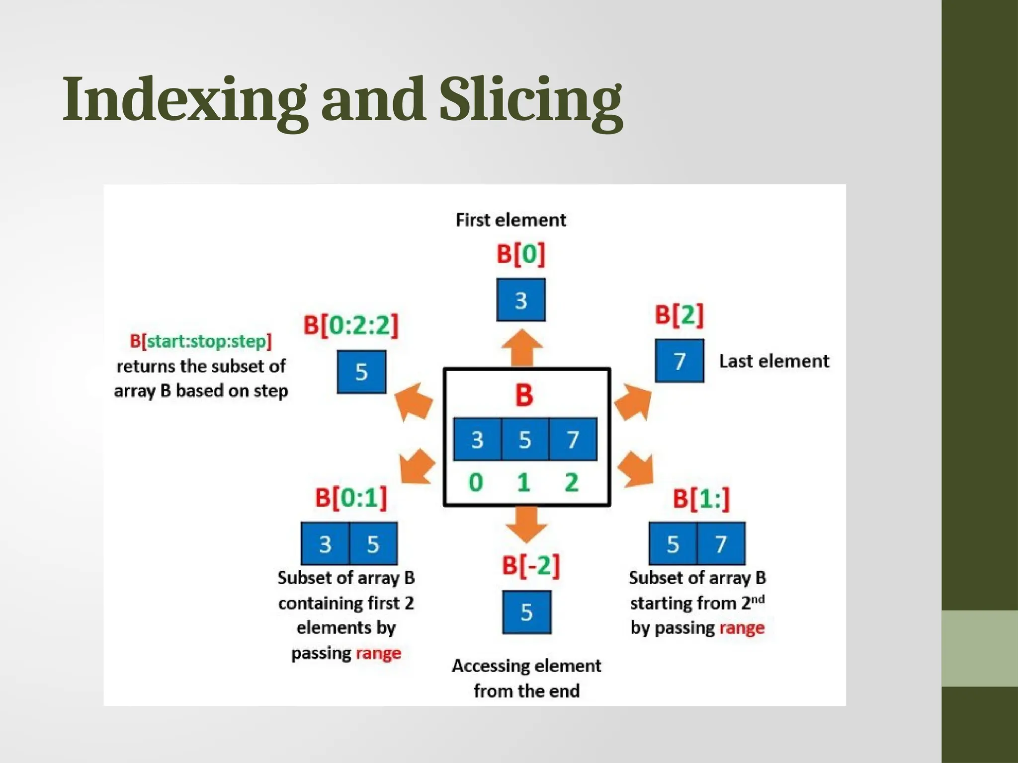
![Indexing & Slicing Indexing import numpy as np arr=([1,2,5,6,7]) print(arr[3]) #6 Slicing import numpy as np arr=([1,2,5,6,7]) print(arr[2:5]) #[5, 6, 7]](https://image.slidesharecdn.com/uniti-datascience-250227192810-b6dbd39e/75/Data-Science-presentation-for-explanation-of-numpy-and-pandas-92-2048.jpg)
![Using np.empty_like( ) • import numpy as np • ary=np.array([13,99,100,34,65,11,66,81,632,44]) • print("Original array: ") • # printing the Numpy array • print(ary) • # Creating an empty Numpy array similar to ary • copy=np.empty_like(ary) • # Now assign ary to copy • copy=ary • print("nCopy of the given array: ") • # printing the copied array • print(copy)](https://image.slidesharecdn.com/uniti-datascience-250227192810-b6dbd39e/75/Data-Science-presentation-for-explanation-of-numpy-and-pandas-97-2048.jpg)
![Using np.copy() function • This function returns an array copy of the given object. Syntax : • numpy.copy(a, order='K', subok=False) # importing Numpy package import numpy as np org_array = np.array([1.54, 2.99, 3.42, 4.87, 6.94, 8.21, 7.65, 10.50, 77.5]) print("Original array: ") print(org_array) # Now copying the org_array to copy_array using np.copy() function copy_array = np.copy(org_array) print("nCopied array: ") # printing the copied Numpy array print(copy_array)](https://image.slidesharecdn.com/uniti-datascience-250227192810-b6dbd39e/75/Data-Science-presentation-for-explanation-of-numpy-and-pandas-99-2048.jpg)
![Using np.copy() function # importing Numpy package import numpy as np org_array = np.array([1.54, 2.99, 3.42, 4.87, 6.94, 8.21, 7.65, 10.50, 77.5]) print("Original array: ") print(org_array) copy_array = np.copy(org_array) print("nCopied array: ") # printing the copied Numpy array print(copy_array)](https://image.slidesharecdn.com/uniti-datascience-250227192810-b6dbd39e/75/Data-Science-presentation-for-explanation-of-numpy-and-pandas-100-2048.jpg)
![Using Assignment Operator import numpy as np org_array = np.array([[99, 22, 33],[44, 77, 66]]) # Copying org_array to copy_array using Assignment operator copy_array = org_array # modifying org_array org_array[1, 2] = 13 # checking if copy_array has remained the same # printing original array print('Original Array: n', org_array) # printing copied array print('nCopied Array: n', copy_array)](https://image.slidesharecdn.com/uniti-datascience-250227192810-b6dbd39e/75/Data-Science-presentation-for-explanation-of-numpy-and-pandas-101-2048.jpg)
![Iterating Arrays • Iterating means going through elements one by one. • As we deal with multi-dimensional arrays in numpy, we can do this using basic for loop of python. • If we iterate on a 1-D array it will go through each element one by one. • Iterate on the elements of the following 1-D array: import numpy as np arr = np.array([1, 2, 3]) for x in arr: print(x) Output: 1 2 3](https://image.slidesharecdn.com/uniti-datascience-250227192810-b6dbd39e/75/Data-Science-presentation-for-explanation-of-numpy-and-pandas-102-2048.jpg)
![Iterating Arrays • Iterating 2-D Arrays • In a 2-D array it will go through all the rows. • If we iterate on a n-D array it will go through (n-1)th dimension one by one. import numpy as np arr = np.array([[1, 2, 3], [4, 5, 6]]) for x in arr: print(x) Output: [1 2 3] [4 5 6]](https://image.slidesharecdn.com/uniti-datascience-250227192810-b6dbd39e/75/Data-Science-presentation-for-explanation-of-numpy-and-pandas-103-2048.jpg)
![Iterating Arrays • To return the actual values, the scalars, we have to iterate the arrays in each dimension. arr = np.array([[1, 2, 3], [4, 5, 6]]) for x in arr: for y in x: print(y) 1 2 3 4 5 6](https://image.slidesharecdn.com/uniti-datascience-250227192810-b6dbd39e/75/Data-Science-presentation-for-explanation-of-numpy-and-pandas-104-2048.jpg)
![Iterating Arrays • Iterating 3-D Arrays • In a 3-D array it will go through all the 2-D arrays. • import numpy as np arr = np.array([[[1, 2, 3], [4, 5, 6]], [[7, 8, 9], [10, 11, 12]]]) for x in arr: print(x) [[1 2 3] [4 5 6]] [[ 7 8 9] [10 11 12]]](https://image.slidesharecdn.com/uniti-datascience-250227192810-b6dbd39e/75/Data-Science-presentation-for-explanation-of-numpy-and-pandas-105-2048.jpg)
![Iterating Arrays • Iterating 3-D Arrays • To return the actual values, the scalars, we have to iterate the arrays in each dimension. import numpy as np arr = np.array([[[1, 2, 3], [4, 5, 6]], [[7, 8, 9], [10, 11, 12]]]) for x in arr: for y in x: for z in y: print(z)](https://image.slidesharecdn.com/uniti-datascience-250227192810-b6dbd39e/75/Data-Science-presentation-for-explanation-of-numpy-and-pandas-106-2048.jpg)
![Iterating Arrays Using nditer() • The function nditer() is a helping function that can be used from very basic to very advanced iterations. • Iterating on Each Scalar Element • In basic for loops, iterating through each scalar of an array we need to use n for loops which can be difficult to write for arrays with very high dimensionality. import numpy as np arr = np.array([[[1, 2], [3, 4]], [[5, 6], [7, 8]]]) for x in np.nditer(arr): print(x) 1 2 3 4 5 6 7 8 1 2 3 4 5 6 7 8 1 2 3 4 5 6 7 8](https://image.slidesharecdn.com/uniti-datascience-250227192810-b6dbd39e/75/Data-Science-presentation-for-explanation-of-numpy-and-pandas-107-2048.jpg)
![Identity • numpy.identity(n, dtype = None) : Return a identity matrix i.e. a square matrix with ones on the main daignol • Parameters: • n : [int] Dimension n x n of output array • dtype : [optional, float(by Default)] Data type of returned array](https://image.slidesharecdn.com/uniti-datascience-250227192810-b6dbd39e/75/Data-Science-presentation-for-explanation-of-numpy-and-pandas-109-2048.jpg)
![Identity array # 2x2 matrix with 1's on main diagonal b = np.identity(2, dtype = float) print("Matrix b : n", b) a = np.identity(4) print("nMatrix a : n", a) Output: Matrix b : [[ 1. 0.] [ 0. 1.]] Matrix a : [[ 1. 0. 0. 0.] [ 0. 1. 0. 0.] [ 0. 0. 1. 0.] [ 0. 0. 0. 1.]]](https://image.slidesharecdn.com/uniti-datascience-250227192810-b6dbd39e/75/Data-Science-presentation-for-explanation-of-numpy-and-pandas-110-2048.jpg)
![eye( ) • numpy.eye(R, C = None, k = 0, dtype = type <‘float’>) : Return a matrix having 1’s on the diagonal and 0’s elsewhere w.r.t. k. • R : Number of rows C : [optional] Number of columns; By default M = N k : [int, optional, 0 by default] Diagonal we require; k>0 means diagonal above main diagonal or vice versa. dtype : [optional, float(by Default)] Data type of returned array.](https://image.slidesharecdn.com/uniti-datascience-250227192810-b6dbd39e/75/Data-Science-presentation-for-explanation-of-numpy-and-pandas-111-2048.jpg)
![Shape of an Array • import numpy as np arr = np.array([[1, 2, 3, 4], [5, 6, 7, 8]]) print(arr.shape) • Output: (2,4)](https://image.slidesharecdn.com/uniti-datascience-250227192810-b6dbd39e/75/Data-Science-presentation-for-explanation-of-numpy-and-pandas-115-2048.jpg)
![Reshape From 1-D to 2-D • import numpy as np arr = np.array([1, 2, 3, 4, 5, 6, 7, 8, 9, 10, 11, 12]) newarr = arr.reshape(4, 3) print(newarr) • Output: • [[ 1 2 3] • [ 4 5 6] • [ 7 8 9] • [10 11 12]]](https://image.slidesharecdn.com/uniti-datascience-250227192810-b6dbd39e/75/Data-Science-presentation-for-explanation-of-numpy-and-pandas-117-2048.jpg)
![Reshape From 1-D to 3-D • The outermost dimension will have 2 arrays that contains 3 arrays, each with 2 elements • import numpy as np arr = np.array([1, 2, 3, 4, 5, 6, 7, 8, 9, 10, 11, 12]) newarr = arr.reshape(2, 3, 2) print(newarr) Output: [[[ 1 2] [ 3 4] [ 5 6]] [[ 7 8] [ 9 10] [11 12]]]](https://image.slidesharecdn.com/uniti-datascience-250227192810-b6dbd39e/75/Data-Science-presentation-for-explanation-of-numpy-and-pandas-118-2048.jpg)
![Can we Reshape into any Shape? • Yes, as long as the elements required for reshaping are equal in both shapes. • We can reshape an 8 elements 1D array into 4 elements in 2 rows 2D array but we cannot reshape it into a 3 elements 3 rows 2D array as that would require 3x3 = 9 elements. import numpy as np arr = np.array([1, 2, 3, 4, 5, 6, 7, 8]) newarr = arr.reshape(3, 3) print(newarr) • Traceback (most recent call last): File "demo_numpy_array_reshape_error.py", line 5, in <module> ValueError: cannot reshape array of size 8 into shape (3,3)](https://image.slidesharecdn.com/uniti-datascience-250227192810-b6dbd39e/75/Data-Science-presentation-for-explanation-of-numpy-and-pandas-119-2048.jpg)
![Flattening the arrays • Flattening array means converting a multidimensional array into a 1D array. • import numpy as np arr = np.array([[1, 2, 3], [4, 5, 6]]) newarr = arr.reshape(-1) print(newarr) • Output: [1 2 3 4 5 6] • There are a lot of functions for changing the shapes of arrays in numpy flatten, ravel and also for rearranging the elements rot90, flip, fliplr, flipud etc. These fall under Intermediate to Advanced section of numpy.](https://image.slidesharecdn.com/uniti-datascience-250227192810-b6dbd39e/75/Data-Science-presentation-for-explanation-of-numpy-and-pandas-120-2048.jpg)

![Series import pandas as pd # Initializing a Series from a list data = [1, 2, 3, 4, 5] series_from_list = pd.Series(data) print(series_from_list) # Initializing a Series from a dictionary data = {'a': 1, 'b': 2, 'c': 3} series_from_dict = pd.Series(data) print(series_from_dict) # Initializing a Series with custom index data = [1, 2, 3, 4, 5] index = ['a', 'b', 'c', 'd', 'e'] series_custom_index = pd.Series(data, index=index) print(series_custom_index) Output 0 1 1 2 2 3 3 4 4 5 dtype: int64 a 1 b 2 c 3 dtype: int64 a 1 b 2 c 3 d 4 e 5 dtype: int64](https://image.slidesharecdn.com/uniti-datascience-250227192810-b6dbd39e/75/Data-Science-presentation-for-explanation-of-numpy-and-pandas-124-2048.jpg)
![Series - Indexing • Each element in a Series has a corresponding index, which can be used to access or manipulate the data. print(series_from_list[0]) print(series_from_dict['b’]) Output 1 2](https://image.slidesharecdn.com/uniti-datascience-250227192810-b6dbd39e/75/Data-Science-presentation-for-explanation-of-numpy-and-pandas-125-2048.jpg)
![Series – Vectorized Operations • Series supports vectorized operations, allowing you to perform arithmetic operations on the entire series efficiently. series_a = pd.Series([1, 2, 3]) series_b = pd.Series([4, 5, 6]) sum_series = series_a + series_b print(sum_series) Output 0 5 1 7 2 9 dtype: int64](https://image.slidesharecdn.com/uniti-datascience-250227192810-b6dbd39e/75/Data-Science-presentation-for-explanation-of-numpy-and-pandas-126-2048.jpg)
![Series – Alignment • When performing operations between two Series objects, Pandas automatically aligns the data based on the index labels. series_a = pd.Series([1, 2, 3], index=['a', 'b', 'c']) series_b = pd.Series([4, 5, 6], index=['b', 'c', 'd']) sum_series = series_a + series_b print(sum_series) Output a NaN b 6.0 c 8.0 d NaN dtype: float64](https://image.slidesharecdn.com/uniti-datascience-250227192810-b6dbd39e/75/Data-Science-presentation-for-explanation-of-numpy-and-pandas-127-2048.jpg)
![Series – NaN Handling • Missing values, represented by NaN (Not a Number), can be handled gracefully in Series operations. series_a = pd.Series([1, 2, 3], index=['a', 'b', 'c']) series_b = pd.Series([4, 5], index=['b', 'c']) sum_series = series_a + series_b print(sum_series) Output a NaN b 6.0 c 8.0 dtype: float64](https://image.slidesharecdn.com/uniti-datascience-250227192810-b6dbd39e/75/Data-Science-presentation-for-explanation-of-numpy-and-pandas-128-2048.jpg)
![DataFrames import pandas as pd # Initializing a DataFrame from a dictionary data = {'Name': ['John', 'Alice', 'Bob'], 'Age': [25, 30, 35], 'City': ['New York', 'Los Angeles', 'Chicago']} df = pd.DataFrame(data) print(df) # Initializing a DataFrame from a list of lists data = [['John', 25, 'New York'], ['Alice', 30, 'Los Angeles'], ['Bob', 35, 'Chicago']] columns = ['Name', 'Age', 'City'] df = pd.DataFrame(data, columns=columns) print(df) Name Age City 0 John 25 New York 1 Alice 30 Los Angeles 2 Bob 35 Chicago Name Age City 0 John 25 New York 1 Alice 30 Los Angeles 2 Bob 35 Chicago](https://image.slidesharecdn.com/uniti-datascience-250227192810-b6dbd39e/75/Data-Science-presentation-for-explanation-of-numpy-and-pandas-131-2048.jpg)
![DataFrames - Indexing • DataFrame provides flexible indexing options, allowing access to rows, columns, or individual elements based on labels or integer positions. # Accessing a column print(df['Name']) # Accessing a row by label print(df.loc[0]) # Accessing a row by integer position print(df.iloc[0]) # Accessing an individual element print(df.at[0, 'Name']) 0 John 1 Alice 2 Bob Name: Name, dtype: object Name John Age 25 City New York Name: 0, dtype: object Name John Age 25 City New York Name: 0, dtype: object John](https://image.slidesharecdn.com/uniti-datascience-250227192810-b6dbd39e/75/Data-Science-presentation-for-explanation-of-numpy-and-pandas-132-2048.jpg)
![DataFrame – Column Operations • Columns in a DataFrame are Series objects, enabling various operations such as arithmetic operations, filtering, and sorting. # Adding a new column df['Salary'] = [50000, 60000, 70000] # Filtering rows based on a condition high_salary_employees = df[df['Salary'] > 60000] print(high_salary_employees) # Sorting DataFrame by a column sorted_df = df.sort_values(by='Age', ascending=False) print(sorted_df)](https://image.slidesharecdn.com/uniti-datascience-250227192810-b6dbd39e/75/Data-Science-presentation-for-explanation-of-numpy-and-pandas-133-2048.jpg)
![DataFrames – Column Operations • Columns in a DataFrame are Series objects, enabling various operations such as arithmetic operations, filtering, and sorting. # Adding a new column df['Salary'] = [50000, 60000, 70000] # Filtering rows based on a condition high_salary_employees = df[df['Salary'] > 60000] print(high_salary_employees) # Sorting DataFrame by a column sorted_df = df.sort_values(by='Age', ascending=False) print(sorted_df) Name Age City Salary 2 Bob 35 Chicago 70000 Name Age City Salary 2 Bob 35 Chicago 70000 1 Alice 30 Los Angeles 60000 0 John 25 New York 50000](https://image.slidesharecdn.com/uniti-datascience-250227192810-b6dbd39e/75/Data-Science-presentation-for-explanation-of-numpy-and-pandas-134-2048.jpg)
![DataFrames – Grouping and Aggregation • DataFrames support group-by operations for summarizing data and applying aggregation functions. # Grouping by a column and calculating mean avg_age_by_city = df.groupby('City')['Age'].mean() print(avg_age_by_city) City Chicago 35.0 Los Angeles 30.0 New York 25.0 Name: Age, dtype: float64](https://image.slidesharecdn.com/uniti-datascience-250227192810-b6dbd39e/75/Data-Science-presentation-for-explanation-of-numpy-and-pandas-136-2048.jpg)
![Index - Creation import pandas as pd data = {'Name': ['Alice', 'Bob', 'Charlie'], 'Age': [25, 30, 35]} df = pd.DataFrame(data, index=['A', 'B', 'C'])](https://image.slidesharecdn.com/uniti-datascience-250227192810-b6dbd39e/75/Data-Science-presentation-for-explanation-of-numpy-and-pandas-139-2048.jpg)
![Re-index • Reindexing is the process of creating a new DataFrame or Series with a different index. • The reindex() method is used for this purpose. import pandas as pd data = {'Name': ['Alice', 'Bob', 'Charlie’], 'Age': [25, 30, 35]} df = pd.DataFrame(data, index=['A', 'B', 'C’]) # Create a new index new_index = ['A', 'B', 'D', 'E'] # Reindex the DataFrame df_reindexed = df.reindex(new_index) df_reindexed](https://image.slidesharecdn.com/uniti-datascience-250227192810-b6dbd39e/75/Data-Science-presentation-for-explanation-of-numpy-and-pandas-140-2048.jpg)
![Drop Entry data = {'Name': ['Alice', 'Bob', 'Charlie'], 'Age': [25, 30, 35]} df = pd.DataFrame(data) df # Drop column newdf = df.drop("Age", axis='columns') newdf](https://image.slidesharecdn.com/uniti-datascience-250227192810-b6dbd39e/75/Data-Science-presentation-for-explanation-of-numpy-and-pandas-142-2048.jpg)
![Selecting Entries – Selecting by Position import pandas as pd data = {'Name': ['Alice', 'Bob', 'Charlie'], 'Age': [25, 30, 35], 'City': ['New York', 'Los Angeles’, 'Chicago']} df = pd.DataFrame(data) # Select the second row df.iloc[1] Selecting data by Position Created DataFrame](https://image.slidesharecdn.com/uniti-datascience-250227192810-b6dbd39e/75/Data-Science-presentation-for-explanation-of-numpy-and-pandas-143-2048.jpg)
![Selecting Entries – Selecting by Condition import pandas as pd data = {'Name': ['Alice', 'Bob', 'Charlie'], 'Age': [25, 30, 35], 'City': ['New York', 'Los Angeles’, 'Chicago']} df = pd.DataFrame(data) # Select rows where Age is greater than 30 df[df['Age'] > 30] Selecting data by Condition Created DataFrame](https://image.slidesharecdn.com/uniti-datascience-250227192810-b6dbd39e/75/Data-Science-presentation-for-explanation-of-numpy-and-pandas-144-2048.jpg)
![Data Alignment import pandas as pd import numpy as np df1 = pd.DataFrame({ 'A': [1, 2, 3], 'B': [4, 5, 6], 'C': [7, 8, 9] }) df2 = pd.DataFrame({ 'A': [10, 11], 'B': [12, 13], 'D': [14, 15] })](https://image.slidesharecdn.com/uniti-datascience-250227192810-b6dbd39e/75/Data-Science-presentation-for-explanation-of-numpy-and-pandas-146-2048.jpg)
![Data Alignment import pandas as pd import numpy as np df1 = pd.DataFrame({ 'A': [1, 2, 3], 'B': [4, 5, 6], 'C': [7, 8, 9] }) df2 = pd.DataFrame({ 'A': [10, 11], 'B': [12, 13], 'D': [14, 15] }) df1_aligned, df2_aligned = df1.align(df2, fill_value=np.nan)](https://image.slidesharecdn.com/uniti-datascience-250227192810-b6dbd39e/75/Data-Science-presentation-for-explanation-of-numpy-and-pandas-147-2048.jpg)
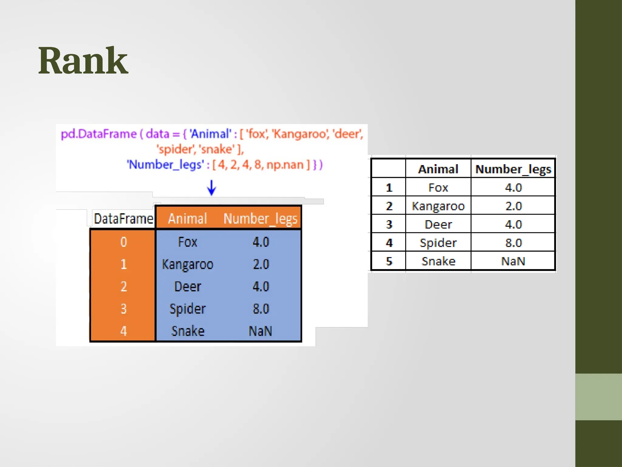
![Rank import numpy as np import pandas as pd df = pd.DataFrame(data={'Animal': ['fox', 'Kangaroo’, 'deer','spider', 'snake’], 'Number_legs': [4, 2, 4, 8, np.nan]}) df](https://image.slidesharecdn.com/uniti-datascience-250227192810-b6dbd39e/75/Data-Science-presentation-for-explanation-of-numpy-and-pandas-149-2048.jpg)
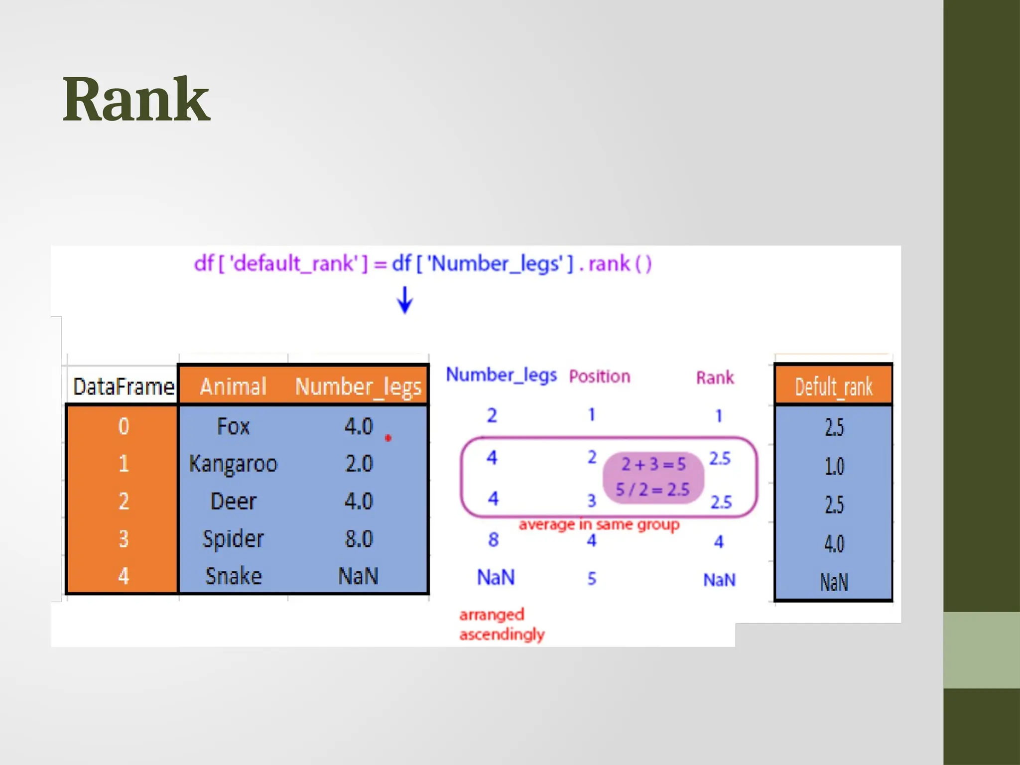
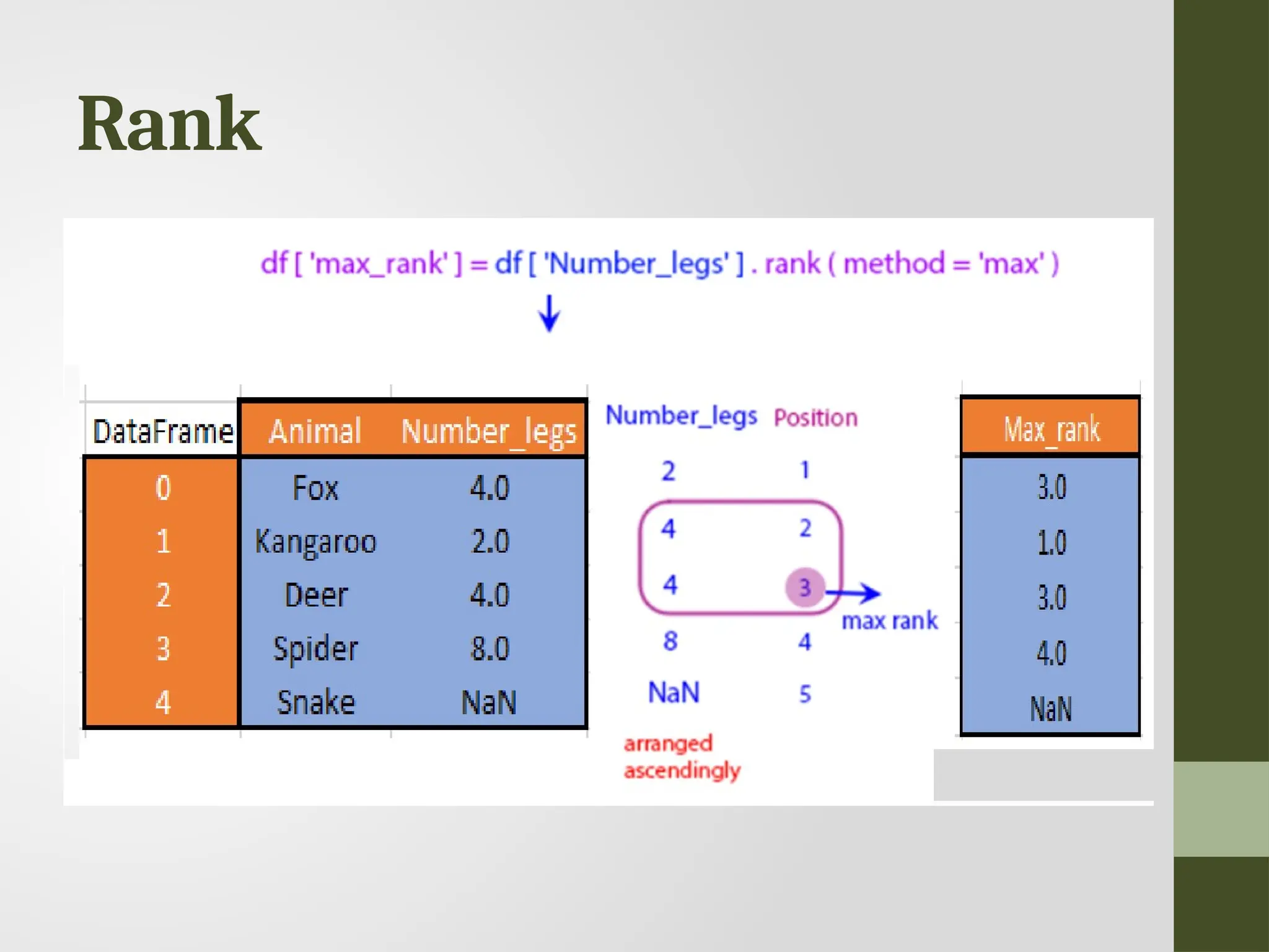
![Rank df['default_rank'] = df['Number_legs'].rank() df['max_rank'] = df['Number_legs'].rank(method='max’) df['NA_bottom’]= df['Number_legs'].rank(na_option='bottom’) df['pct_rank'] = df['Number_legs'].rank(pct=True) df](https://image.slidesharecdn.com/uniti-datascience-250227192810-b6dbd39e/75/Data-Science-presentation-for-explanation-of-numpy-and-pandas-151-2048.jpg)
![Sort import pandas as pd age_list = [['Afghanistan', 1952, 8425333, 'Asia'], ['Australia', 1957, 9712569, 'Oceania'], ['Brazil', 1962, 76039390, 'Americas'], ['China', 1957, 637408000, 'Asia'], ['France', 1957, 44310863, 'Europe'], ['India', 1952, 3.72e+08, 'Asia'], ['United States', 1957, 171984000, 'Americas']] df = pd.DataFrame(age_list, columns=['Country', 'Year', 'Population', 'Continent']) df](https://image.slidesharecdn.com/uniti-datascience-250227192810-b6dbd39e/75/Data-Science-presentation-for-explanation-of-numpy-and-pandas-157-2048.jpg)
![Sort import pandas as pd age_list = [['Afghanistan', 1952, 8425333, 'Asia'], ['Australia', 1957, 9712569, 'Oceania'], ['Brazil', 1962, 76039390, 'Americas'], ['China', 1957, 637408000, 'Asia'], ['France', 1957, 44310863, 'Europe'], ['India', 1952, 3.72e+08, 'Asia'], ['United States', 1957, 171984000, 'Americas']] df = pd.DataFrame(age_list, columns=['Country', 'Year’, 'Population', 'Continent']) df](https://image.slidesharecdn.com/uniti-datascience-250227192810-b6dbd39e/75/Data-Science-presentation-for-explanation-of-numpy-and-pandas-158-2048.jpg)
![Sort by Ascending Order import pandas as pd age_list = [['Afghanistan', 1952, 8425333, 'Asia'], ['Australia', 1957, 9712569, 'Oceania'], ['Brazil', 1962, 76039390, 'Americas'], ['China', 1957, 637408000, 'Asia'], ['France', 1957, 44310863, 'Europe'], ['India', 1952, 3.72e+08, 'Asia'], ['United States', 1957, 171984000, 'Americas']] df = pd.DataFrame(age_list, columns=['Country', 'Year’, 'Population', 'Continent’]) df.sort_values(by=['Country’]) # sorting in Ascending Order df](https://image.slidesharecdn.com/uniti-datascience-250227192810-b6dbd39e/75/Data-Science-presentation-for-explanation-of-numpy-and-pandas-159-2048.jpg)
![Sort by Descending Order import pandas as pd age_list = [['Afghanistan', 1952, 8425333, 'Asia'], ['Australia', 1957, 9712569, 'Oceania'], ['Brazil', 1962, 76039390, 'Americas'], ['China', 1957, 637408000, 'Asia'], ['France', 1957, 44310863, 'Europe'], ['India', 1952, 3.72e+08, 'Asia'], ['United States', 1957, 171984000, 'Americas']] df = pd.DataFrame(age_list, columns=['Country', 'Year’, 'Population', 'Continent’]) df.sort_values(by=['Population'], ascending=False) # sorting in Descending Order df](https://image.slidesharecdn.com/uniti-datascience-250227192810-b6dbd39e/75/Data-Science-presentation-for-explanation-of-numpy-and-pandas-160-2048.jpg)
![Sort by Descending Order import pandas as pd age_list = [['Afghanistan', 1952, 8425333, 'Asia'], ['Australia', 1957, 9712569, 'Oceania'], ['Brazil', 1962, 76039390, 'Americas'], ['China', 1957, 637408000, 'Asia'], ['France', 1957, 44310863, 'Europe'], ['India', 1952, 3.72e+08, 'Asia'], ['United States', 1957, 171984000, 'Americas']] df = pd.DataFrame(age_list, columns=['Country', 'Year’, 'Population', 'Continent’]) df.sort_values(by=['Population'], ascending=False) # sorting in Descending Order df](https://image.slidesharecdn.com/uniti-datascience-250227192810-b6dbd39e/75/Data-Science-presentation-for-explanation-of-numpy-and-pandas-161-2048.jpg)