Download to read offline

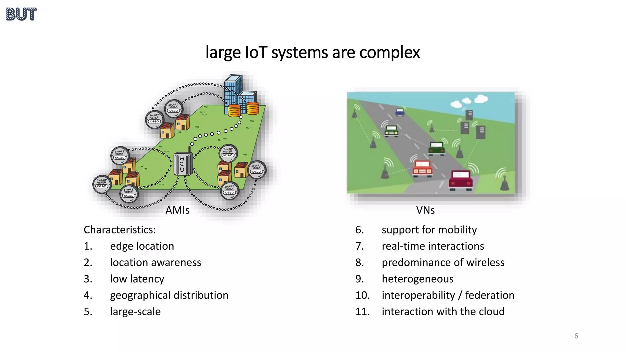
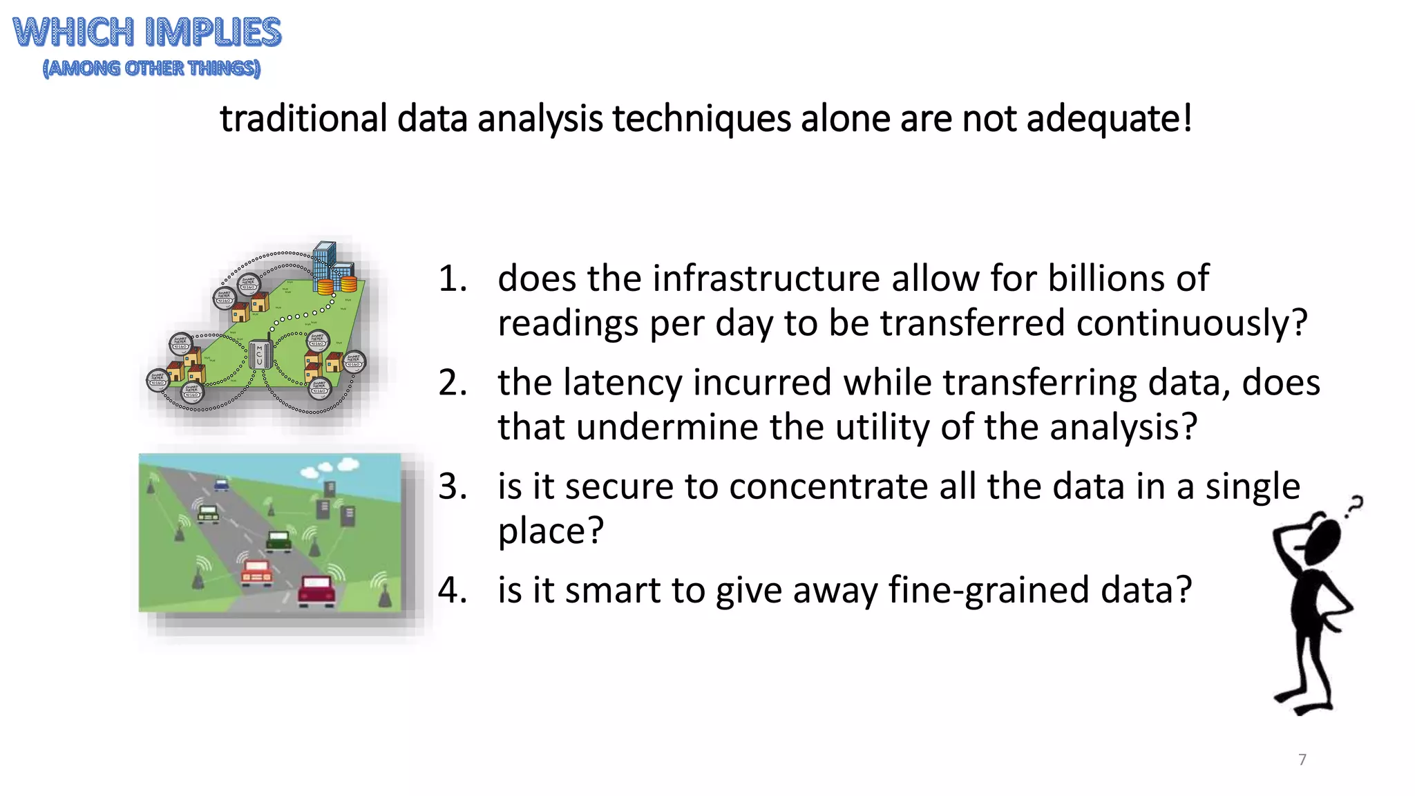
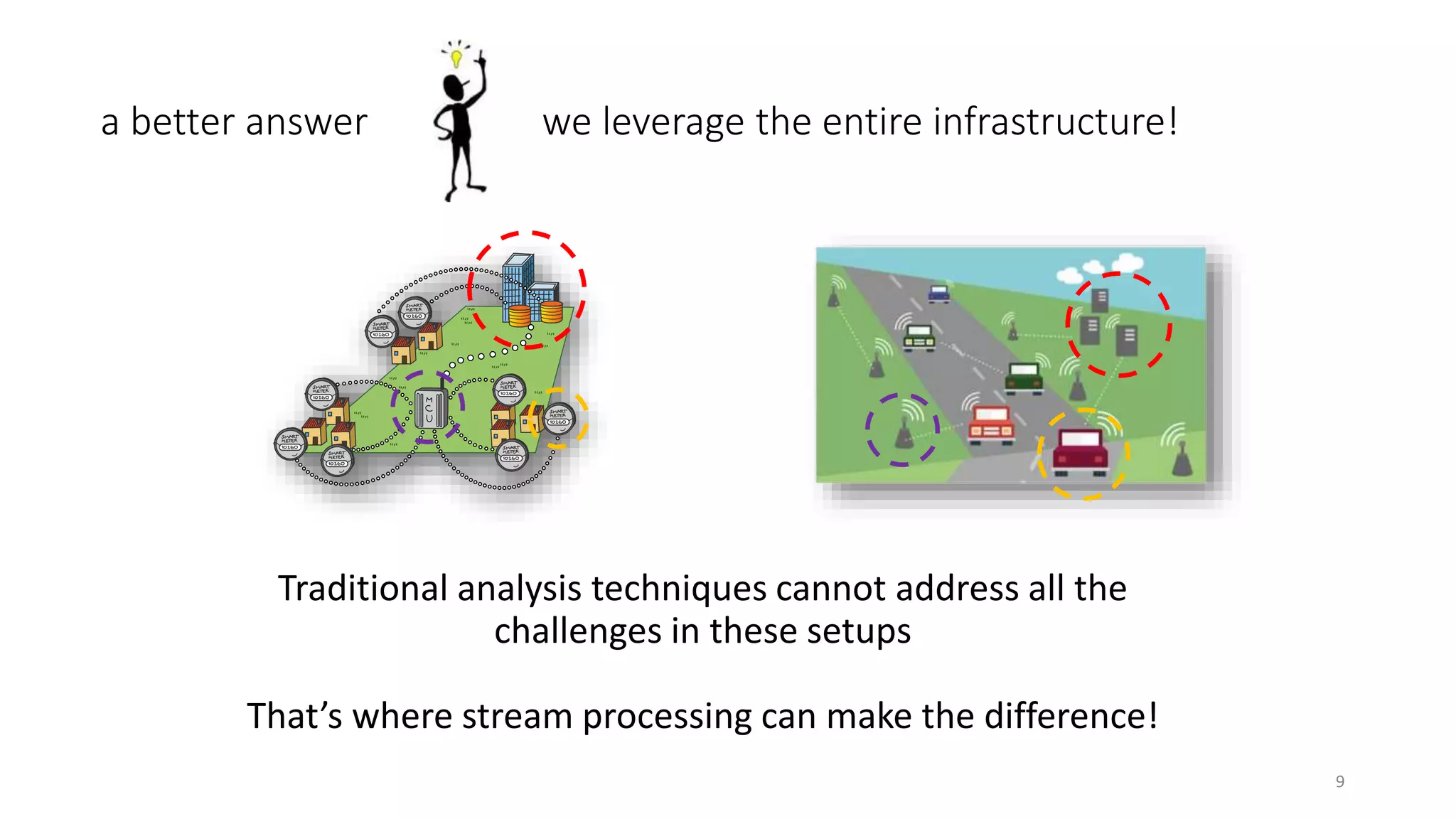
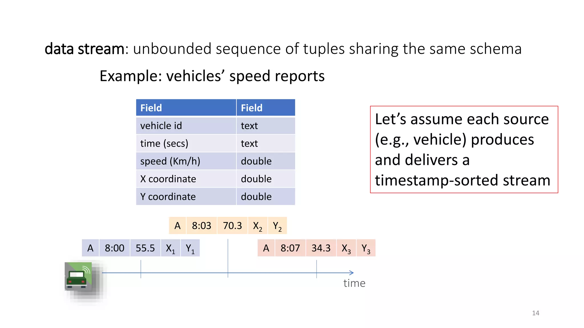
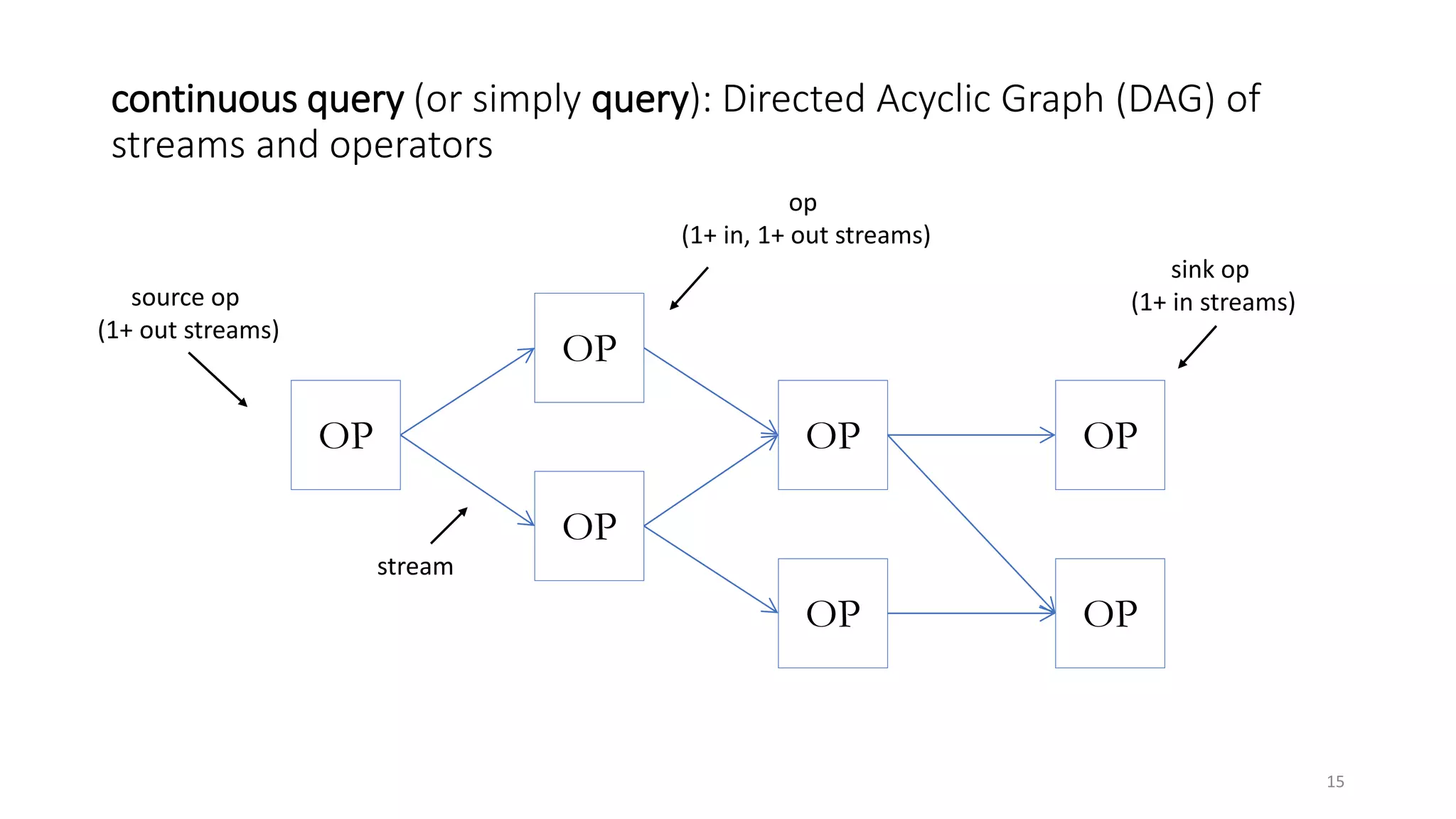
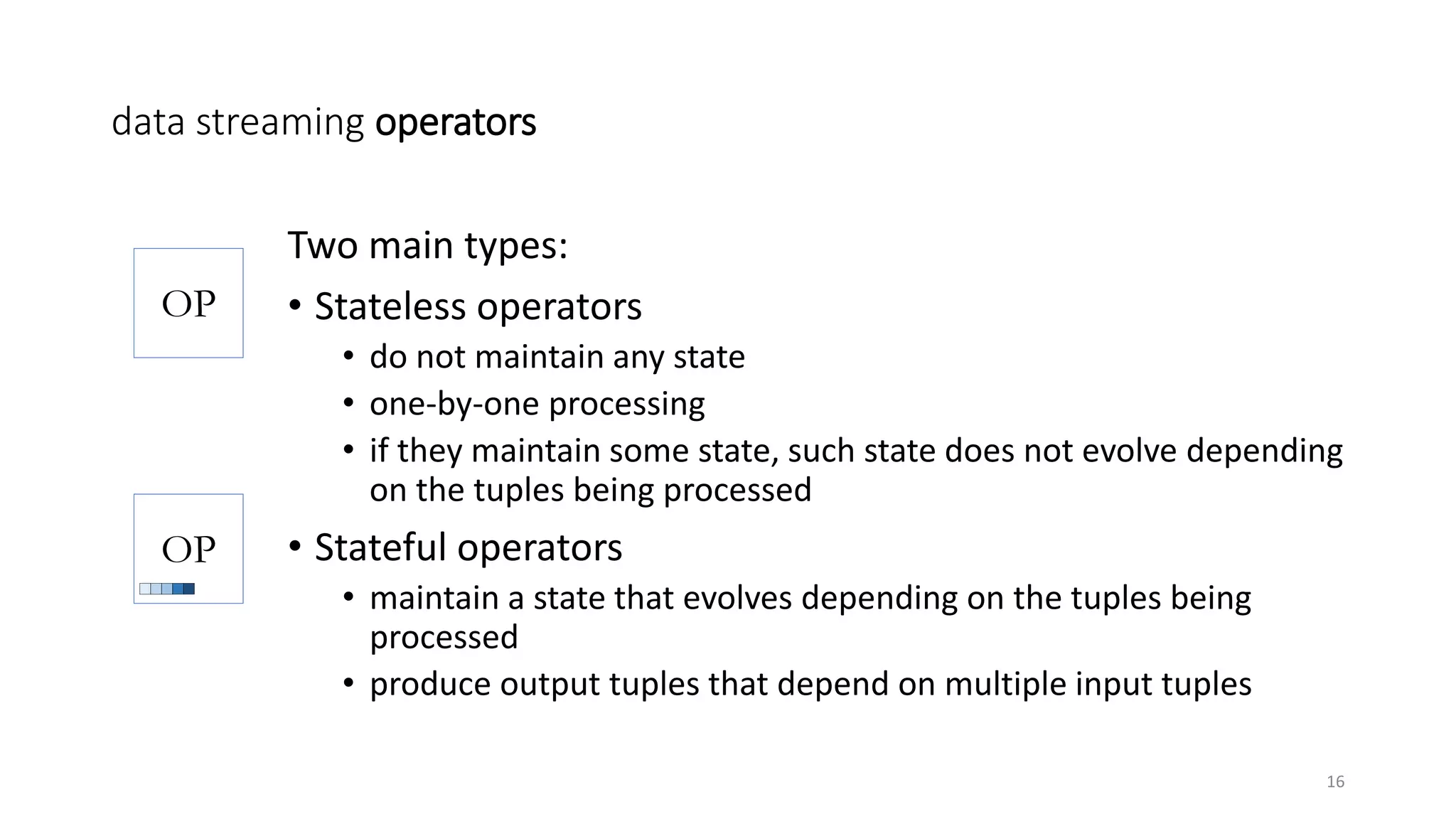
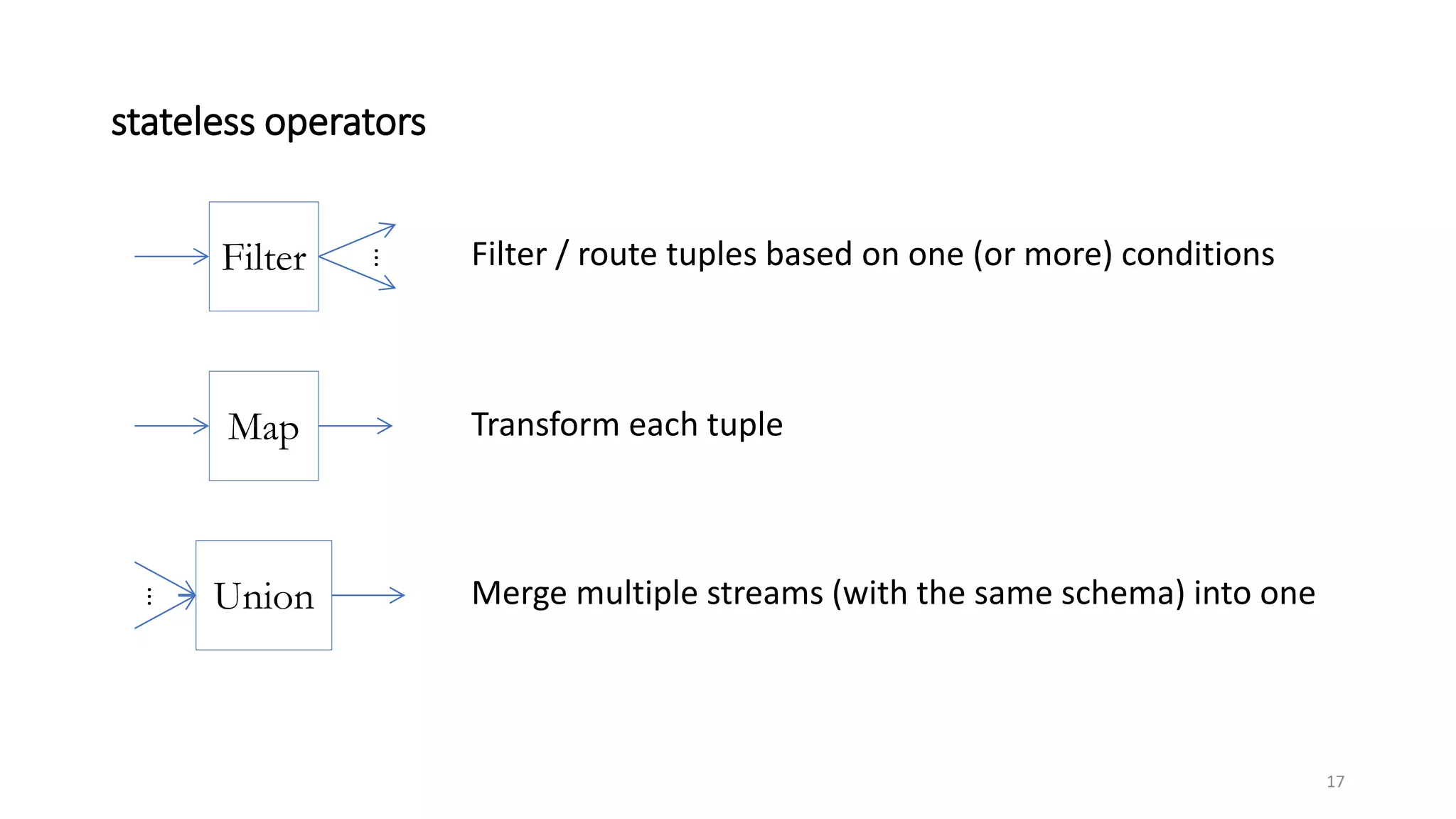
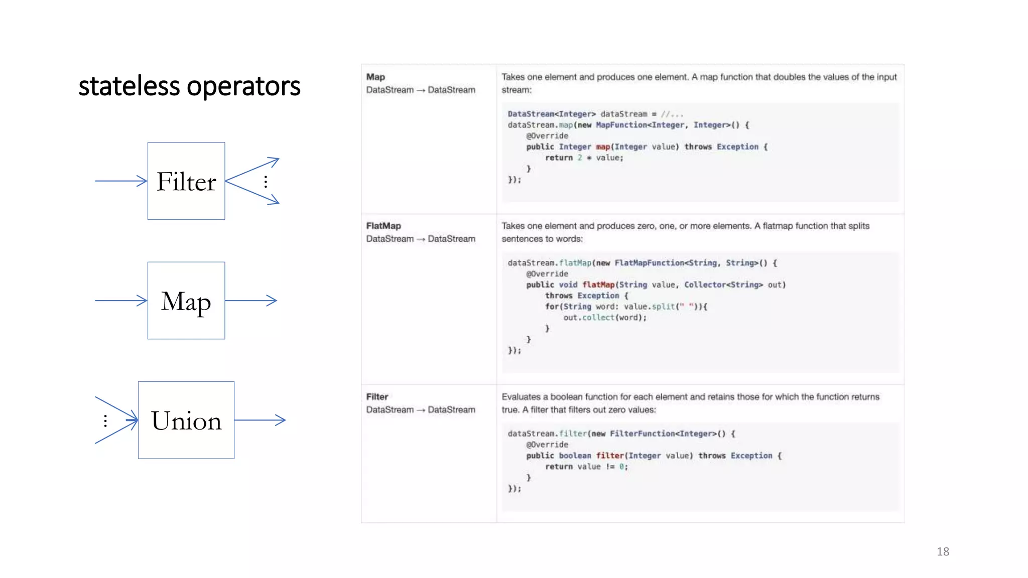
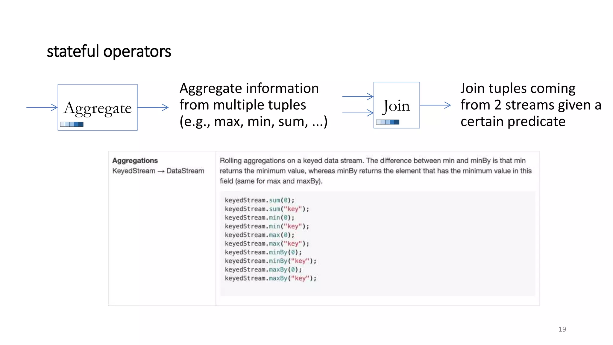
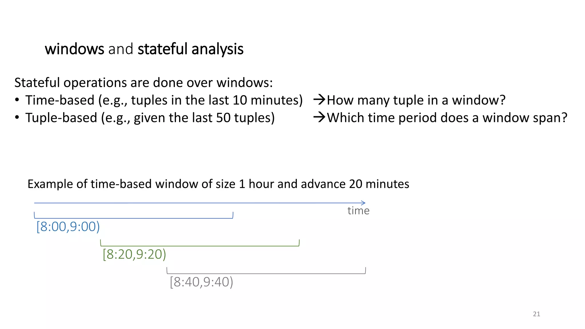
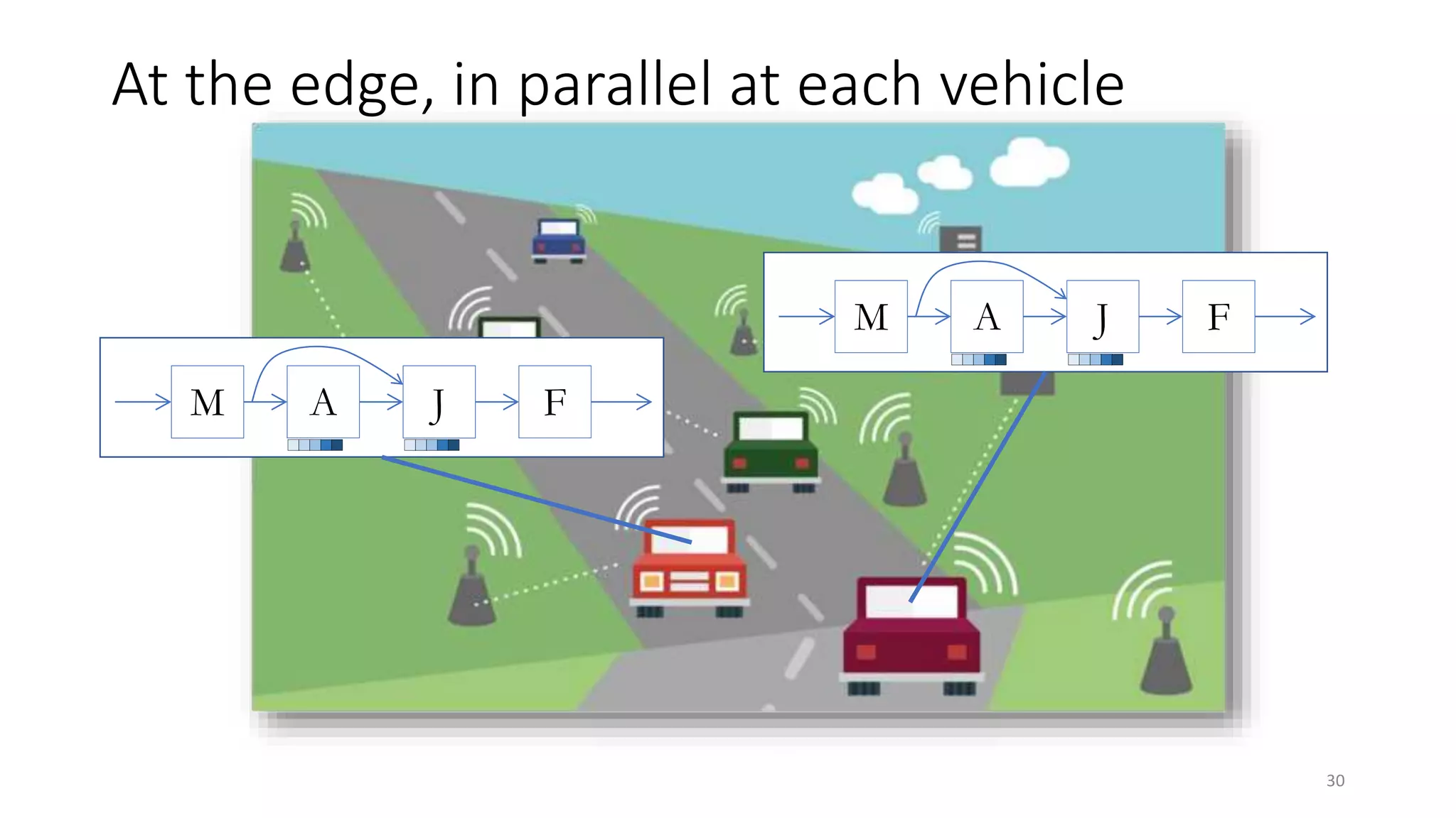
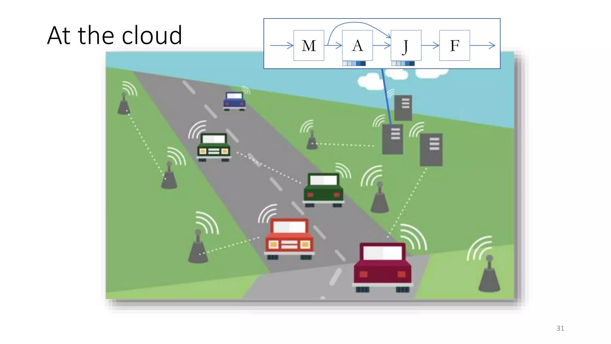
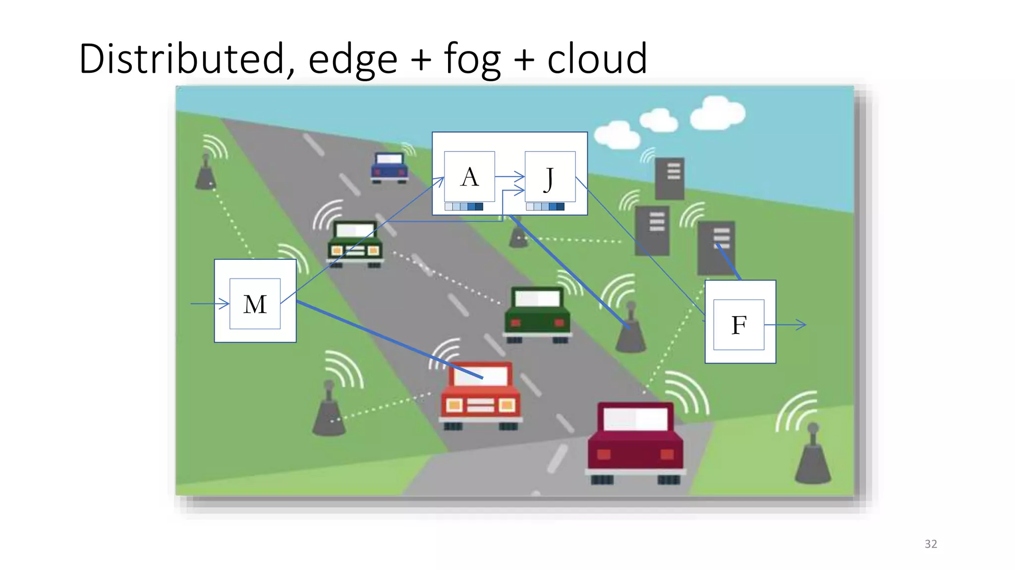
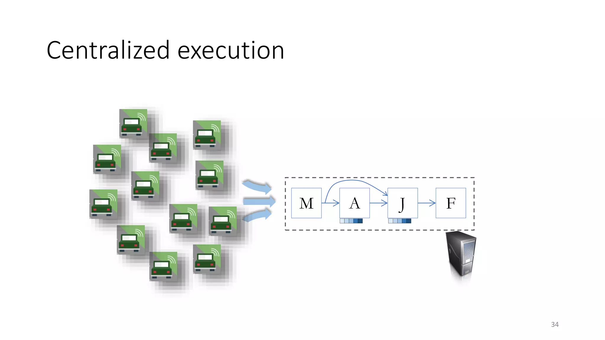
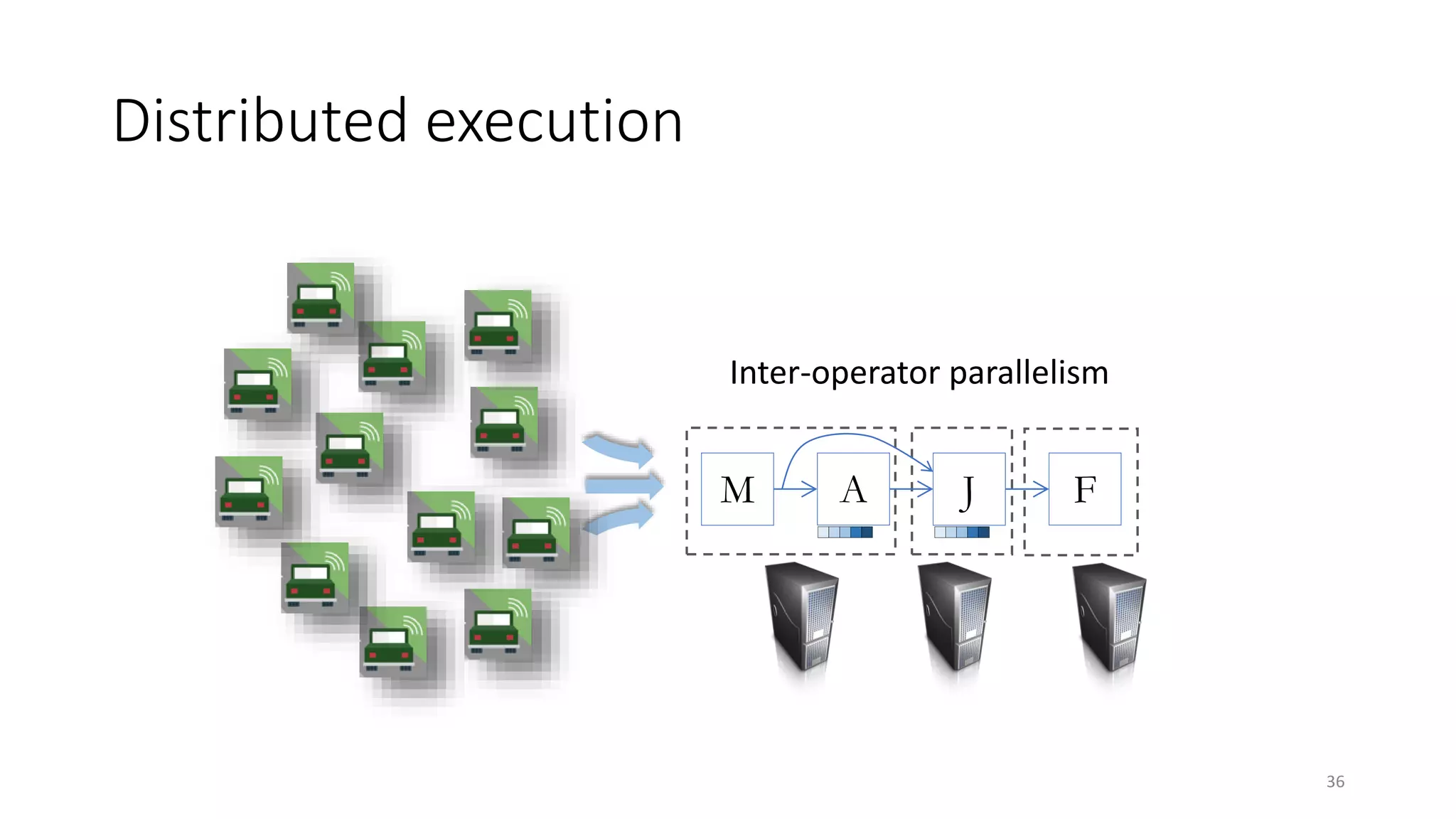
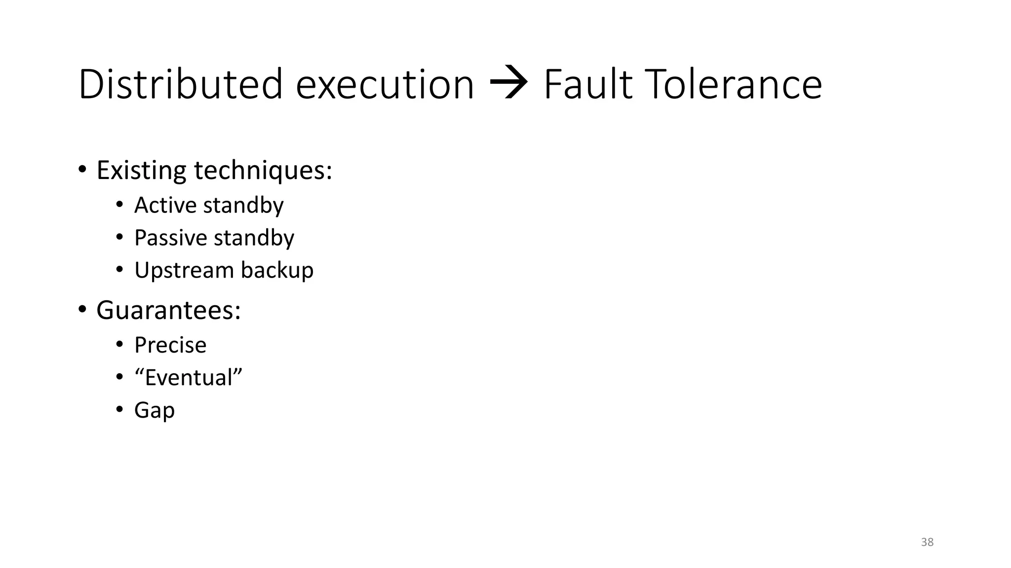
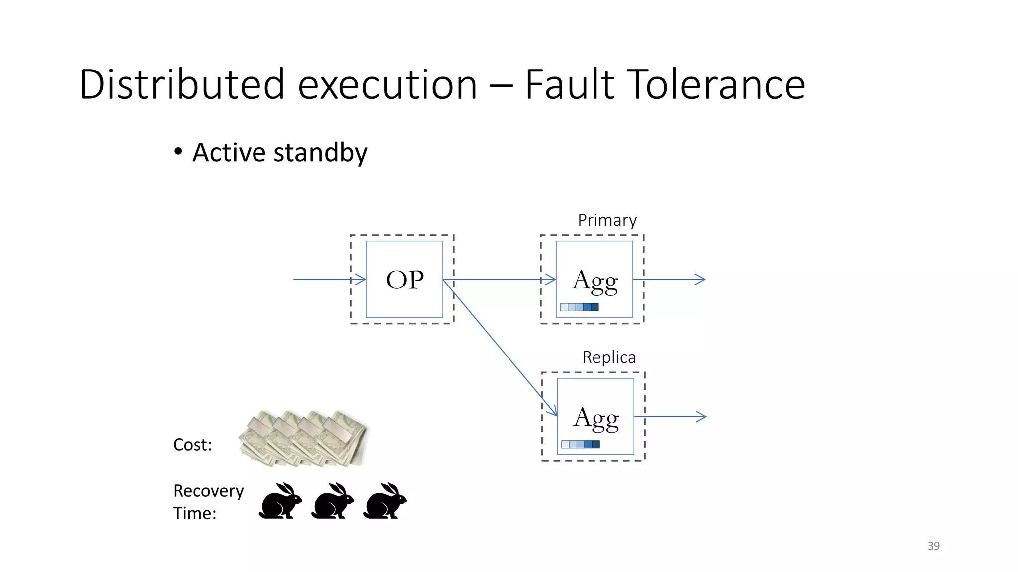
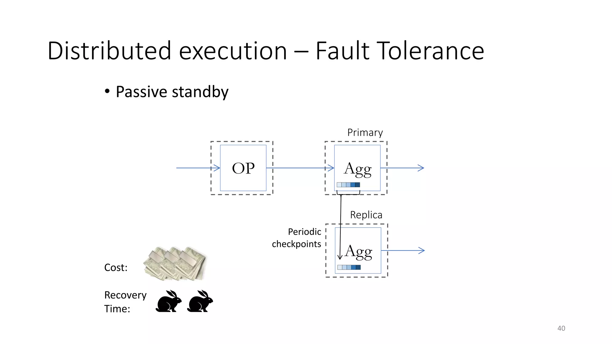
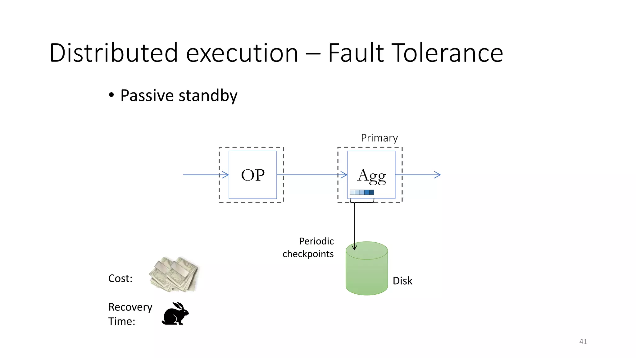
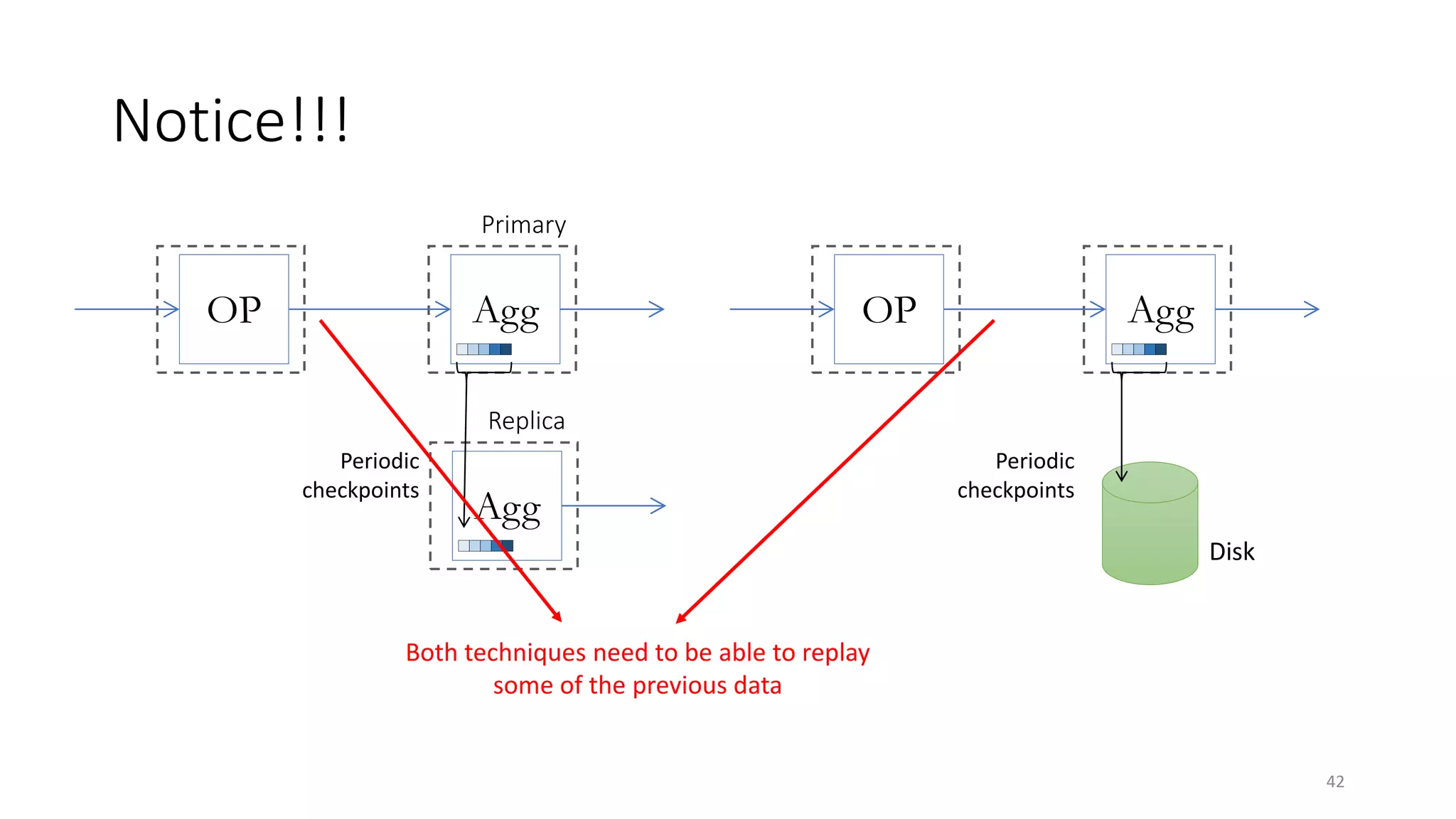
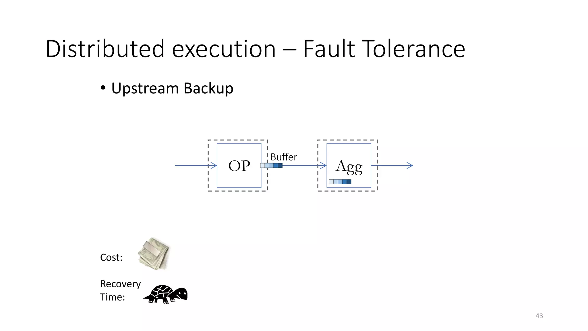
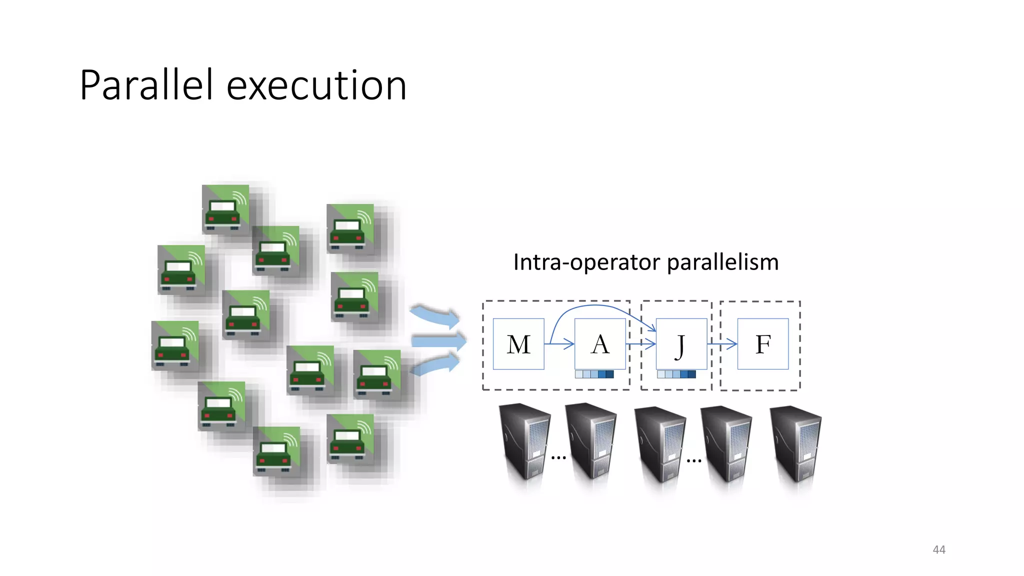
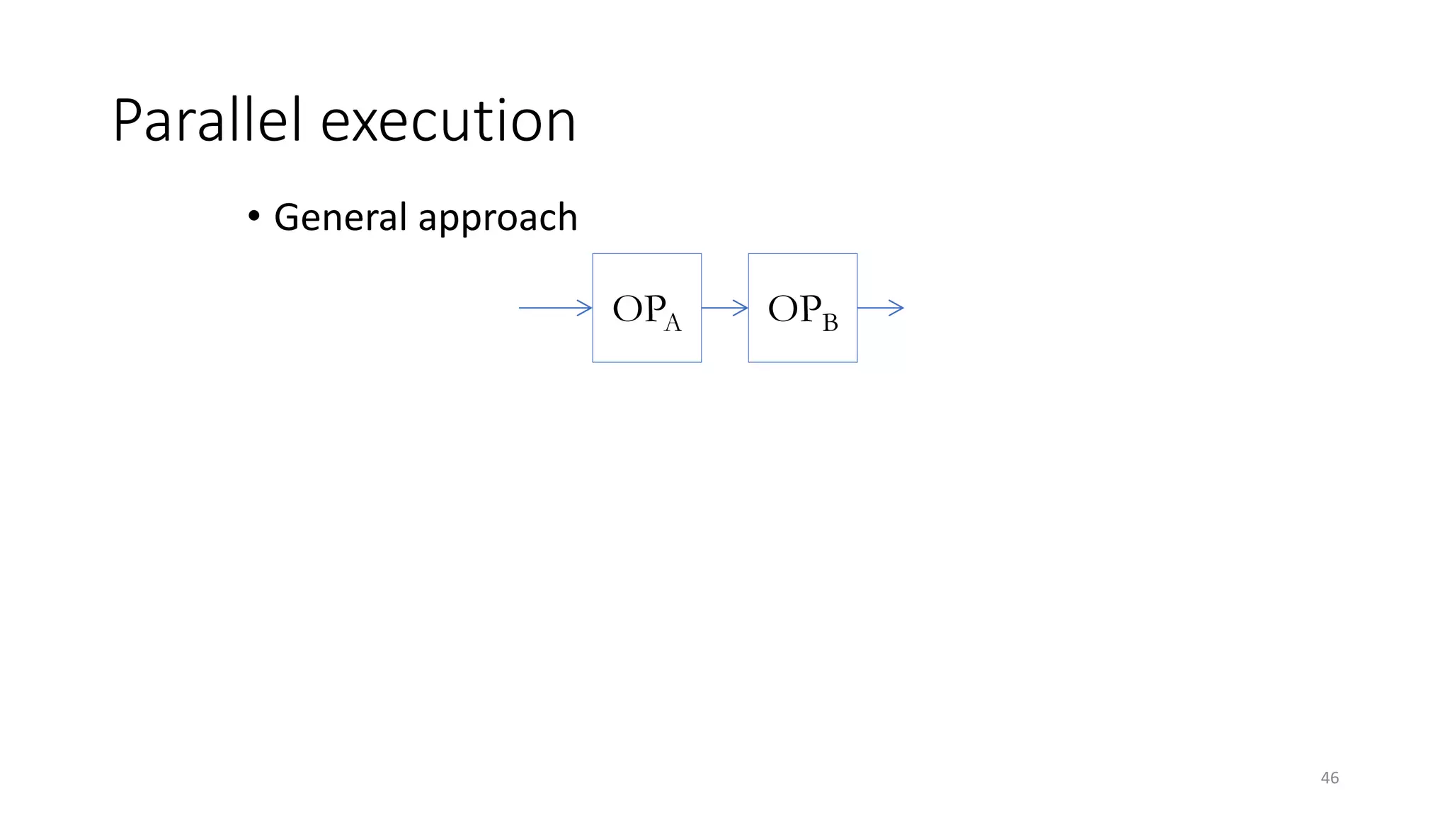
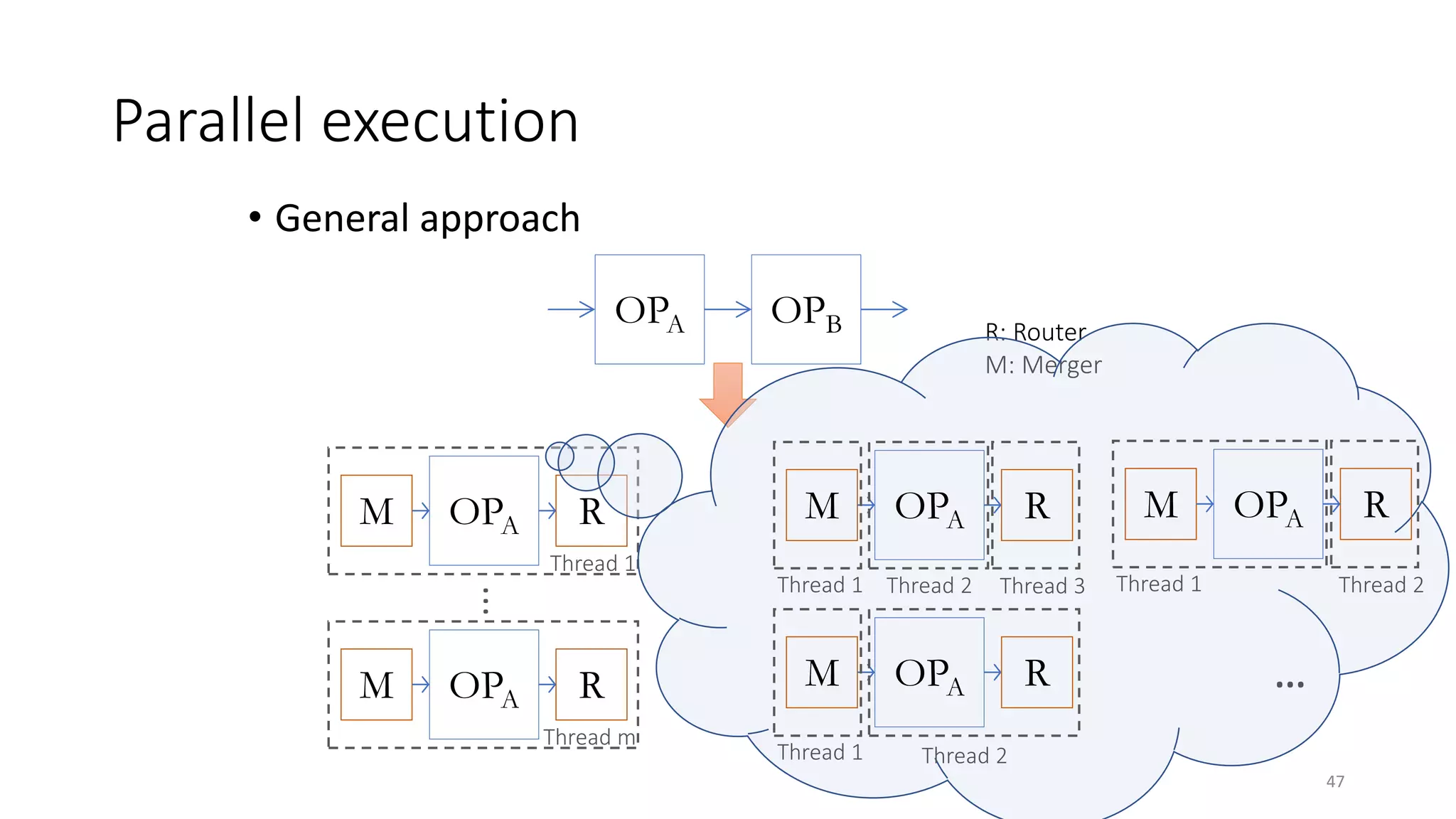
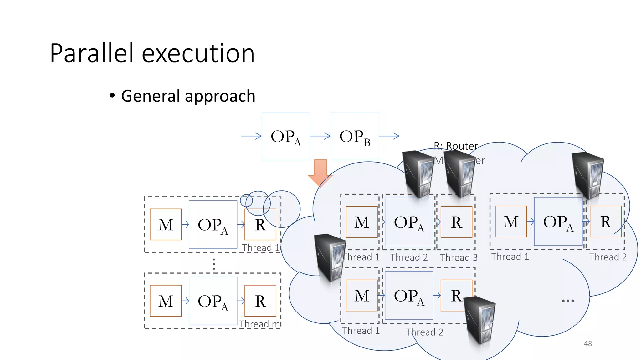
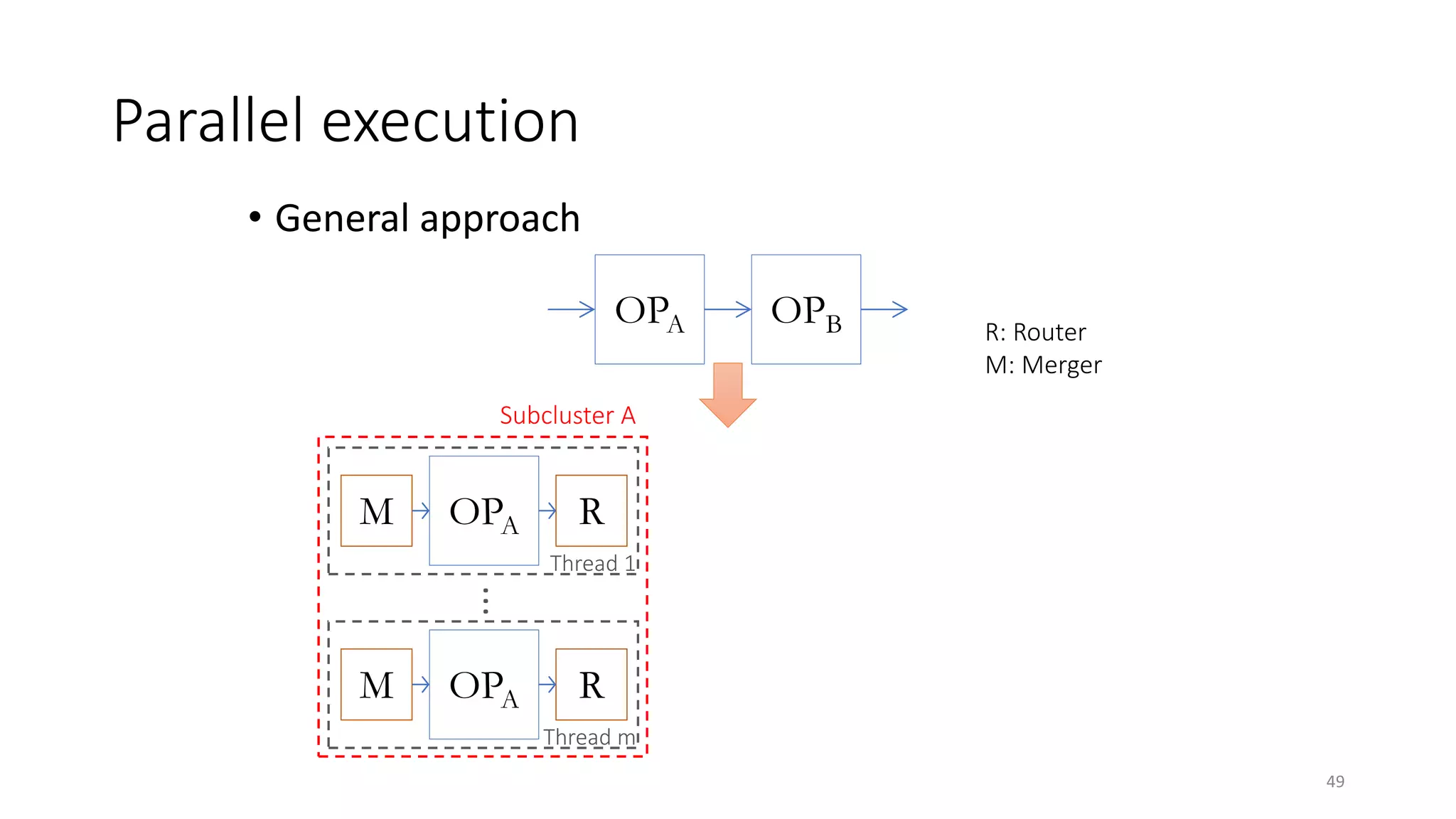
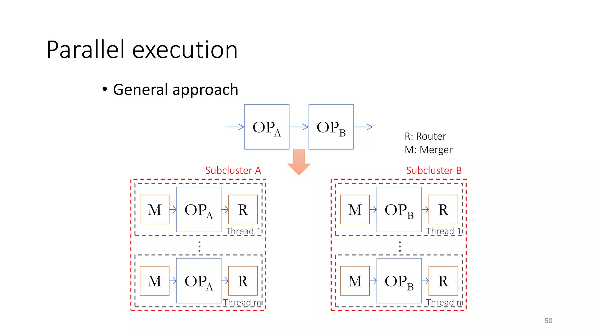
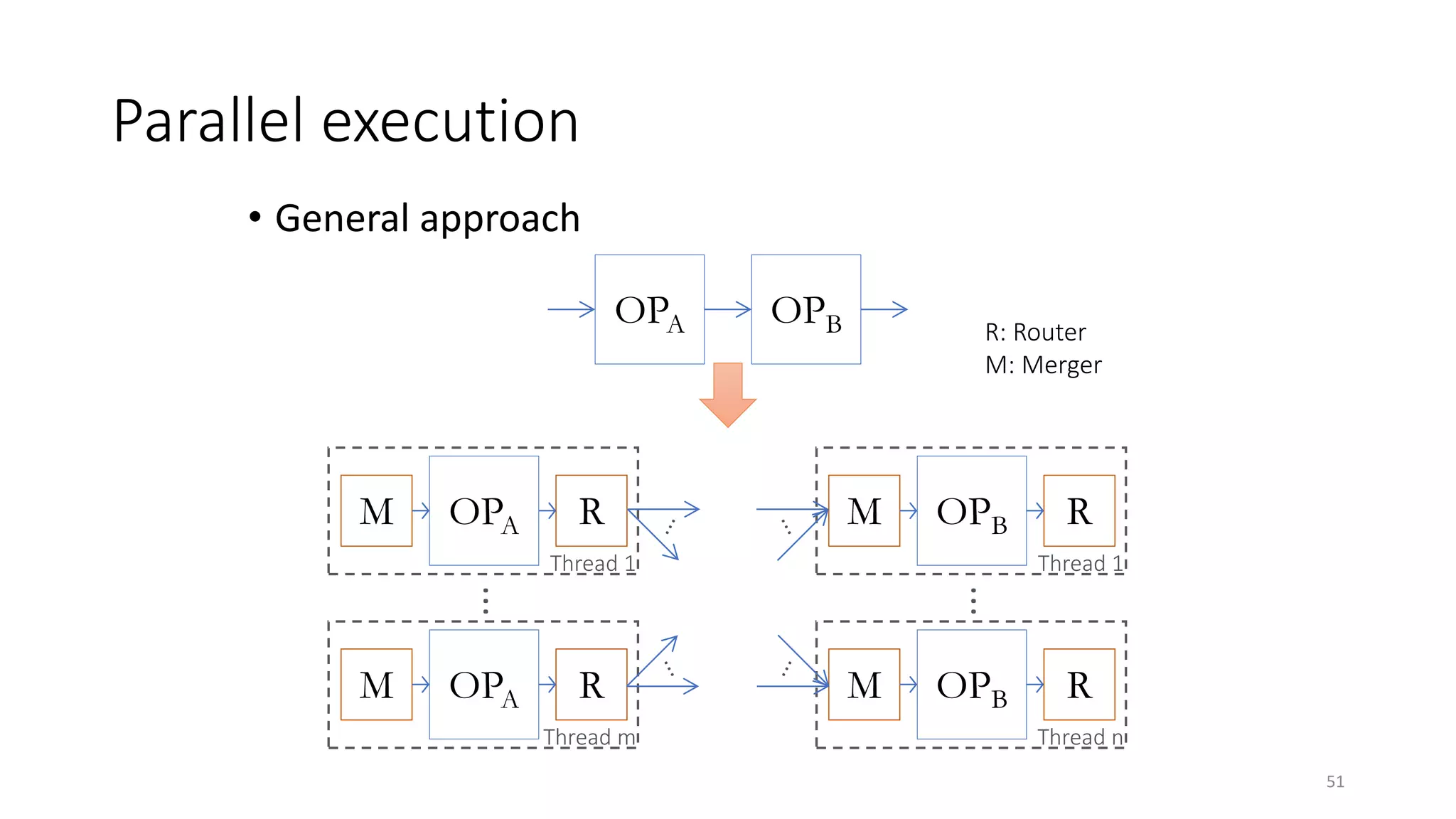
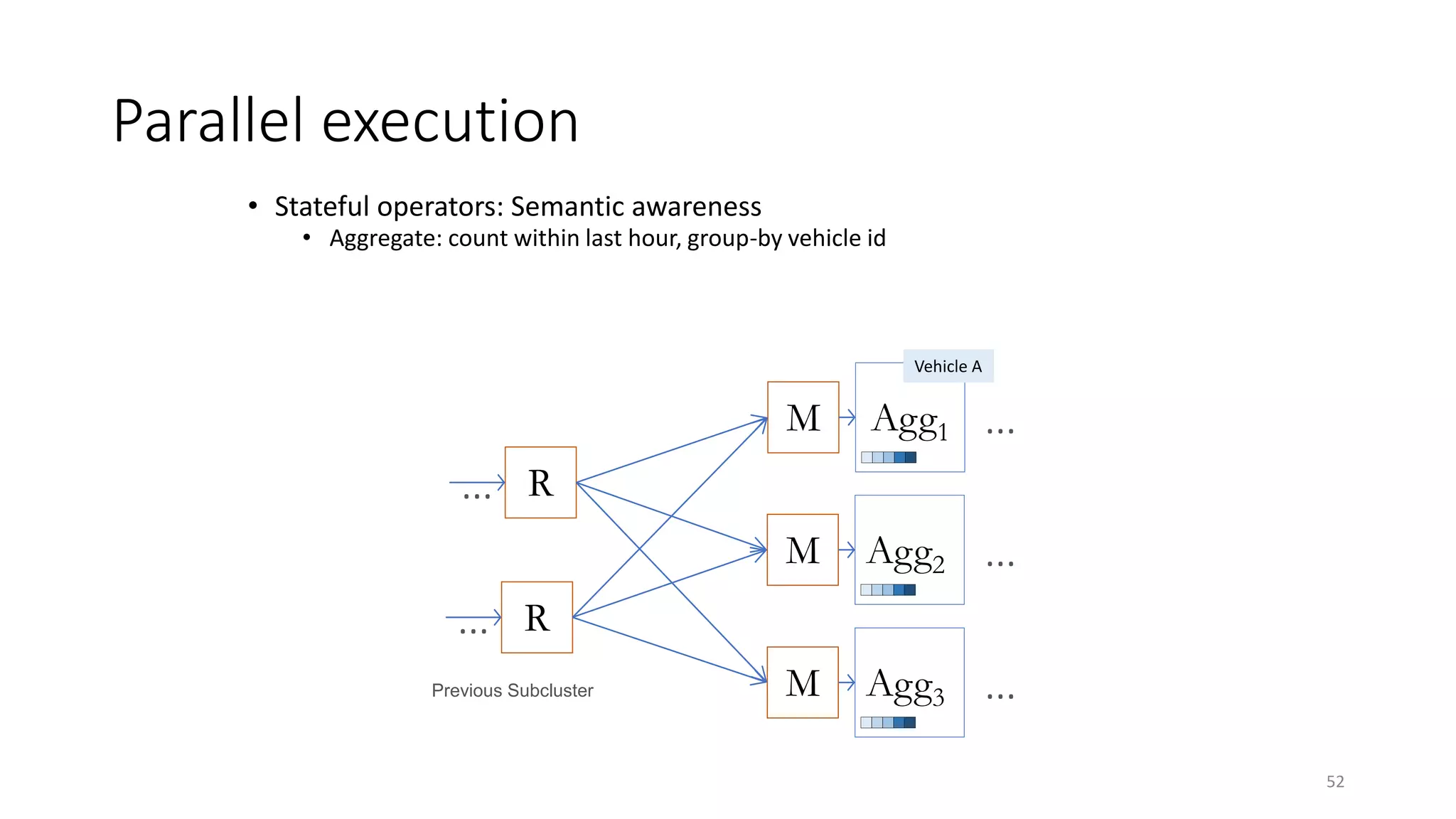
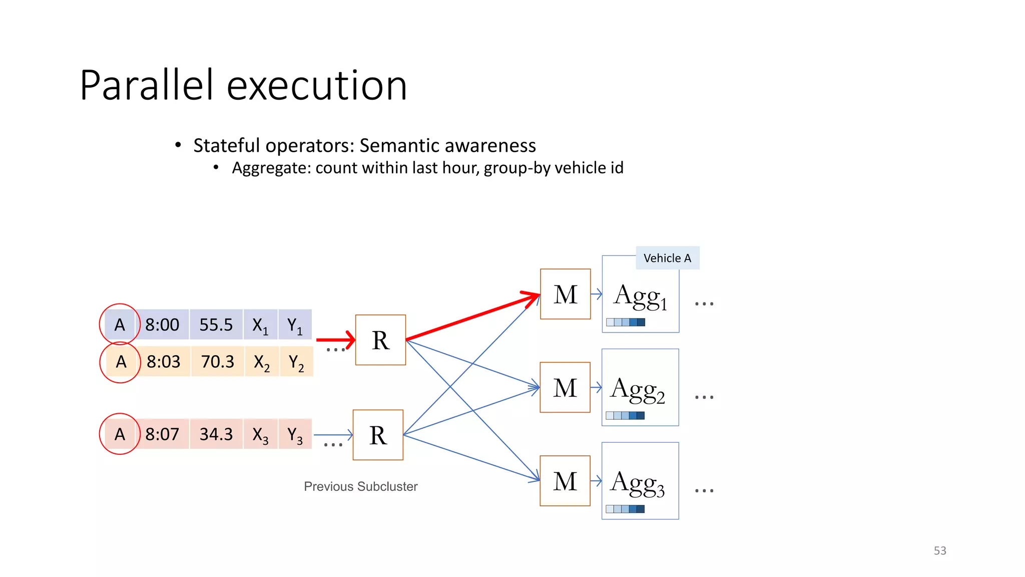
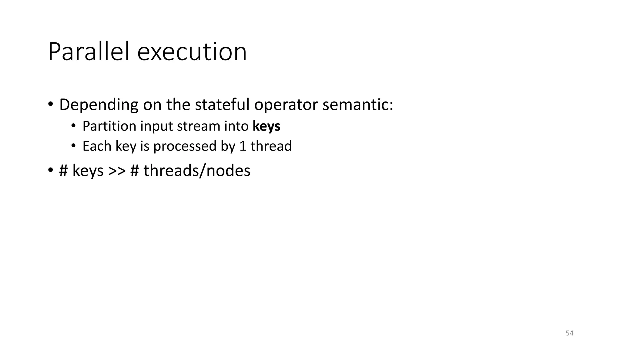
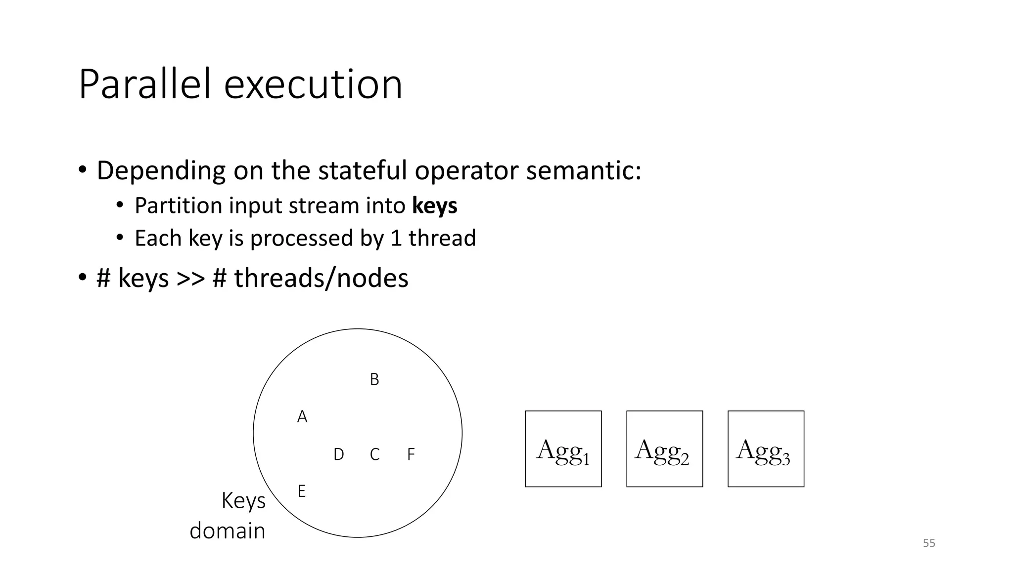
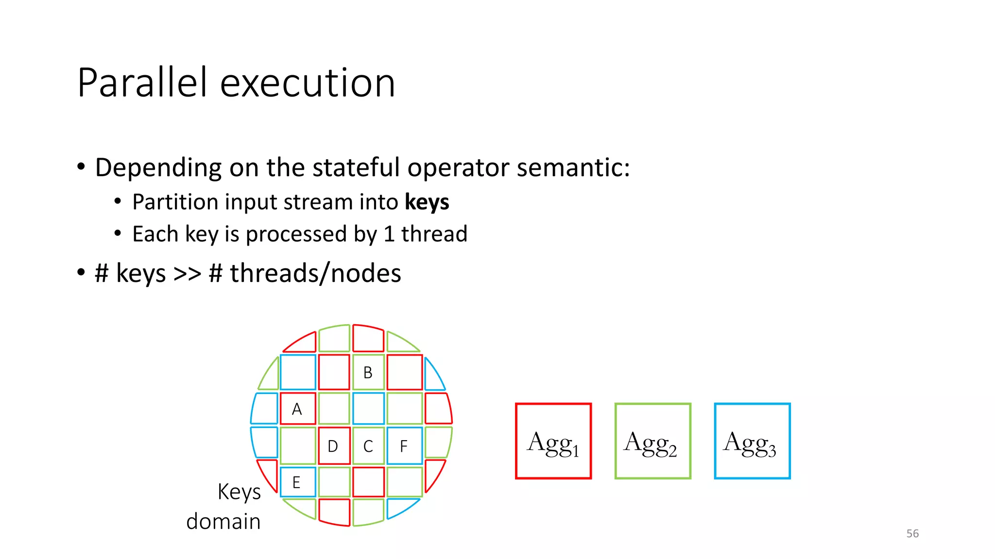
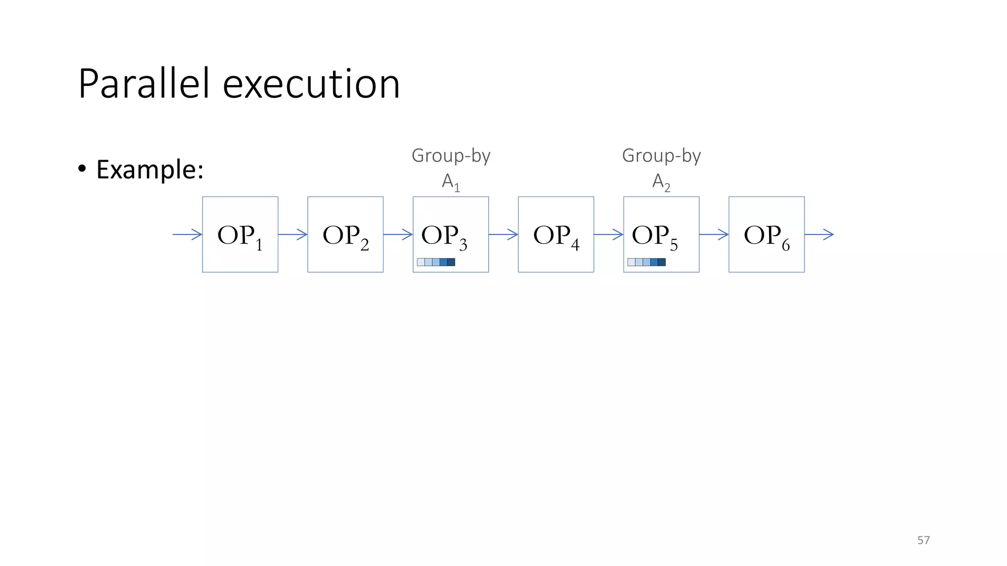
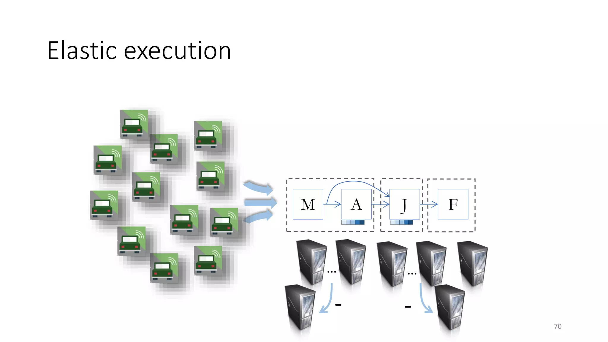
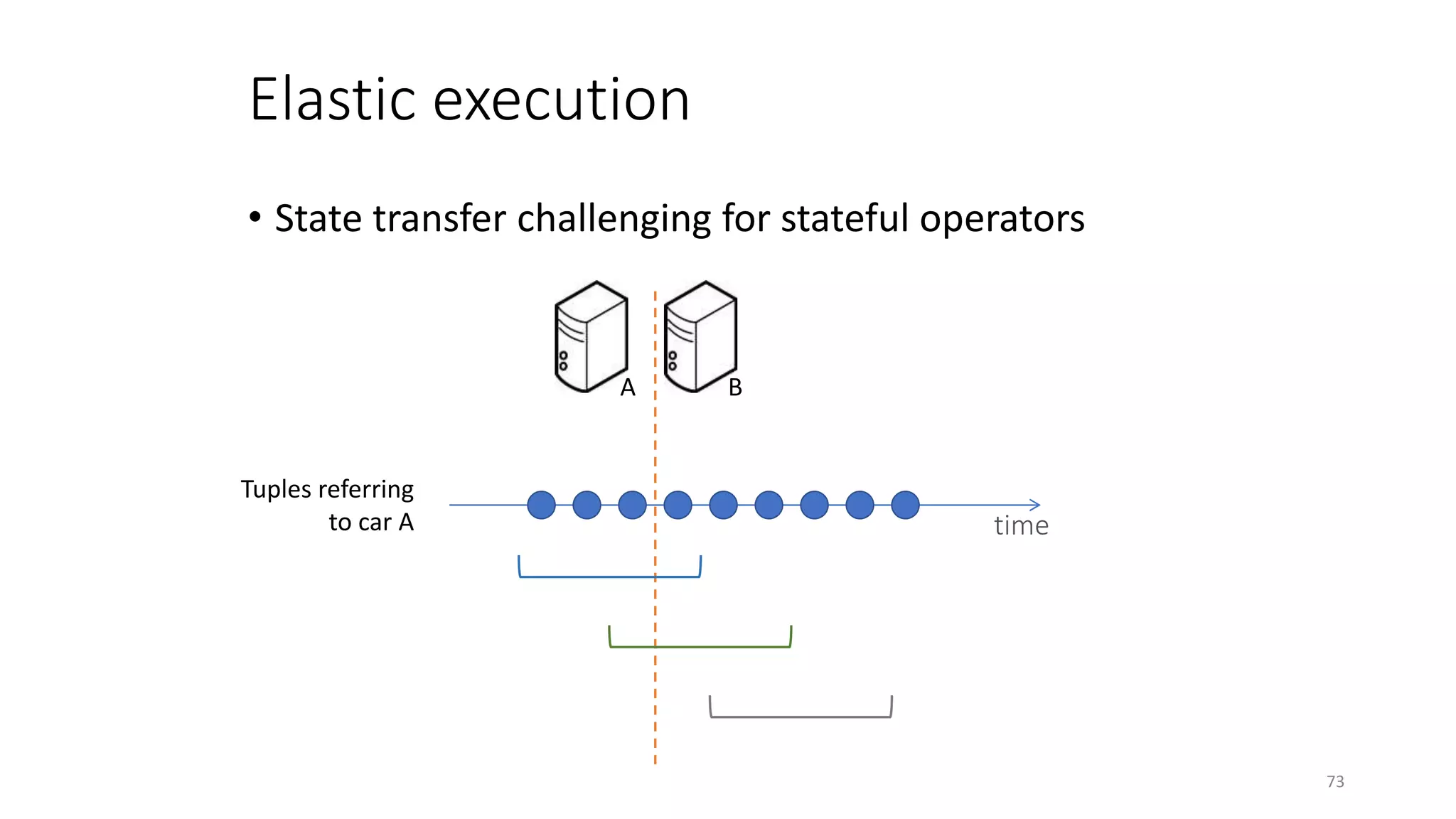
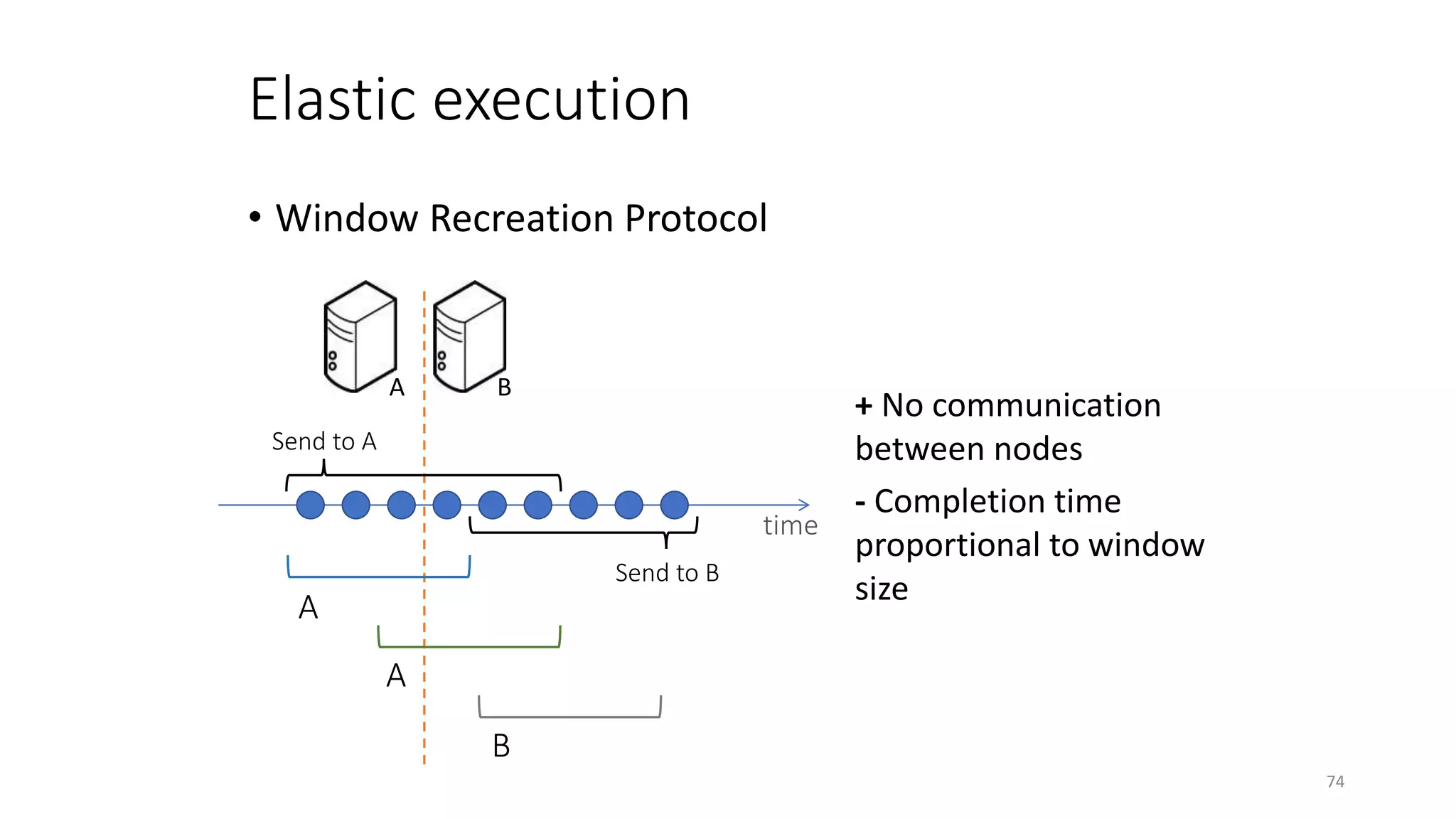
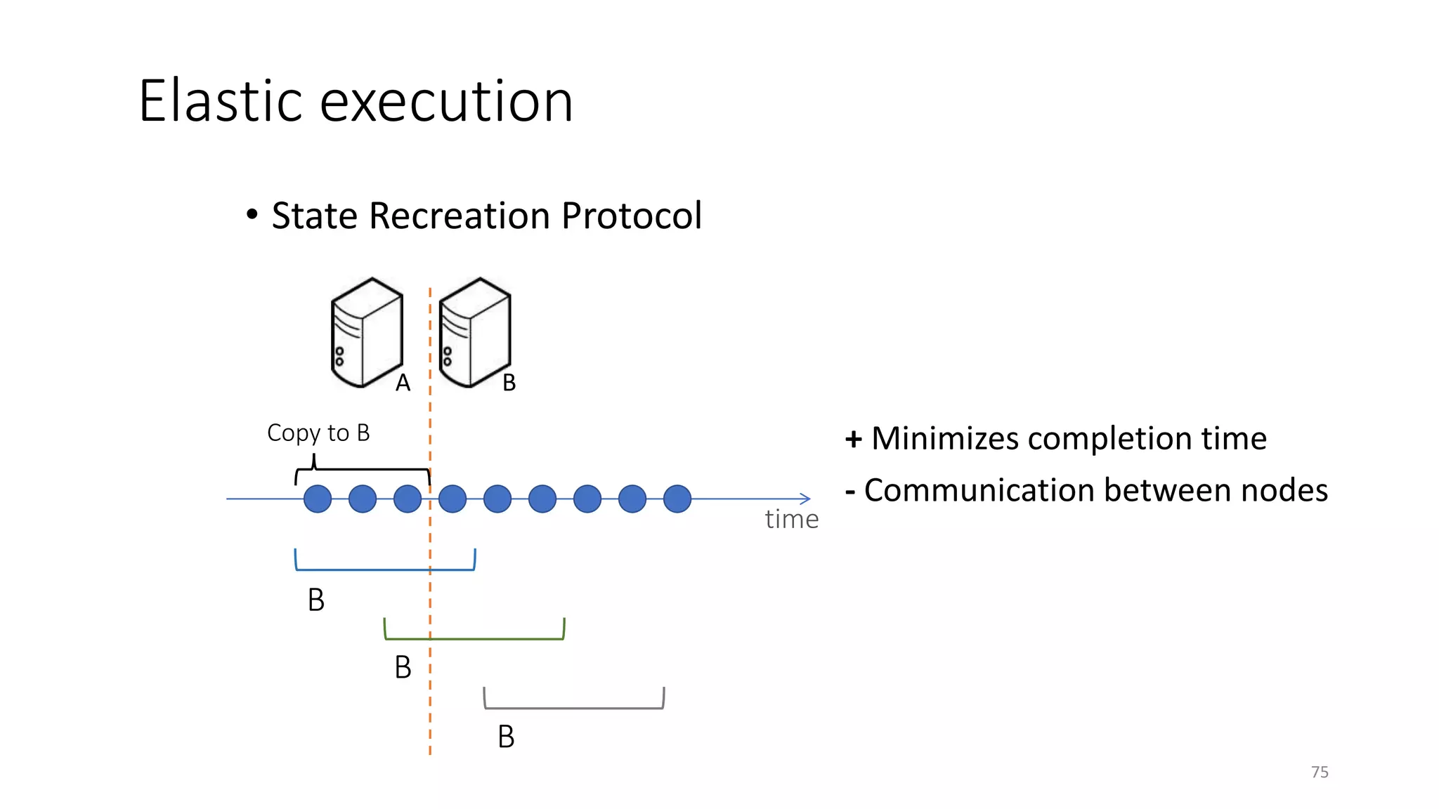
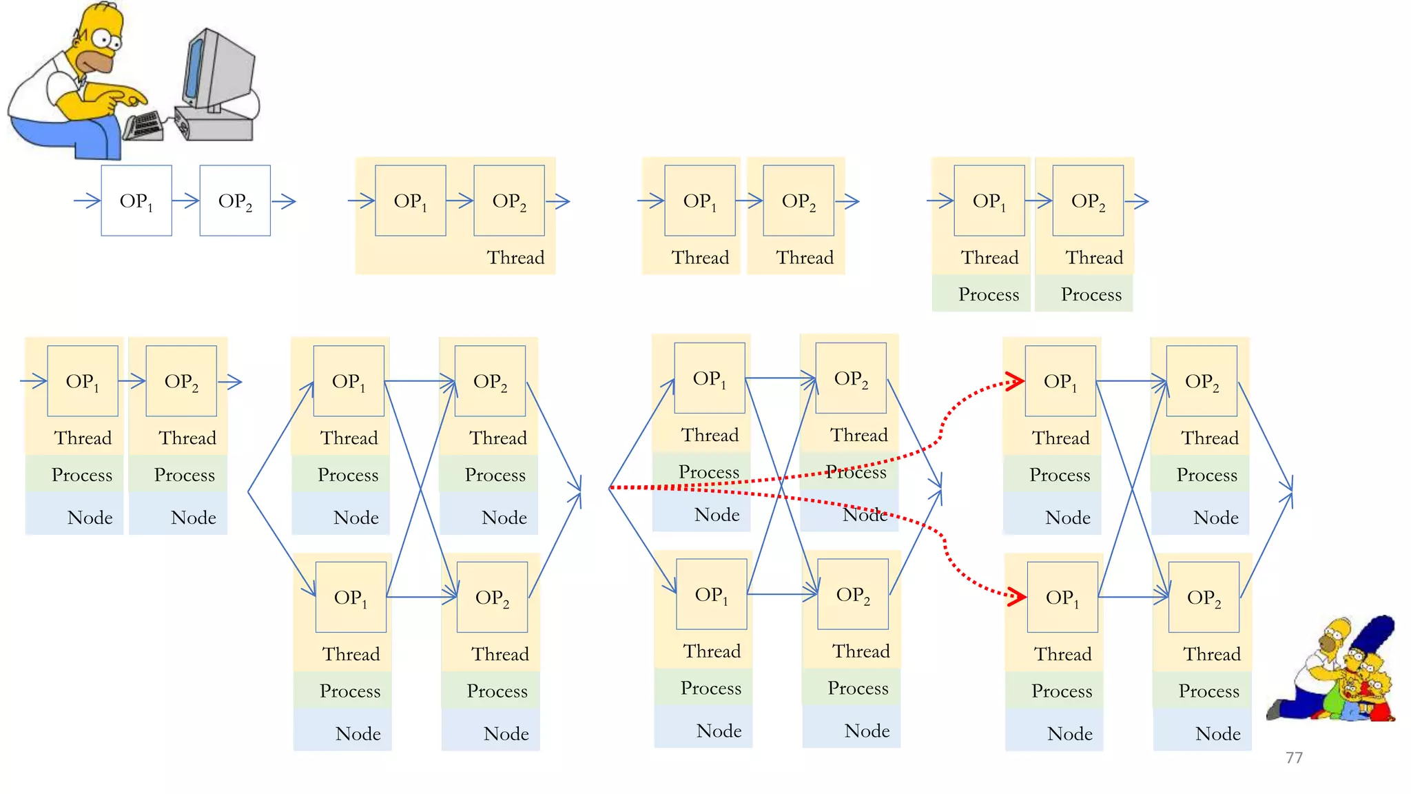

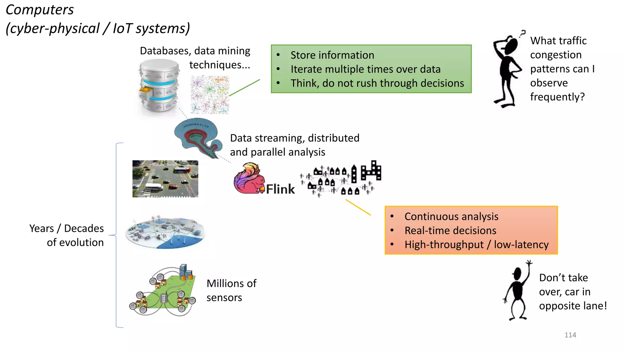


The document provides an overview of stream processing, highlighting its significance in managing complex IoT systems and data streaming techniques that surpass traditional data analysis methods. It discusses key concepts such as edge location, real-time interactions, and various types of operators used in stream processing architectures. Additionally, it addresses the challenges of distributed execution, fault tolerance, and correctness guarantees in stream processing environments.