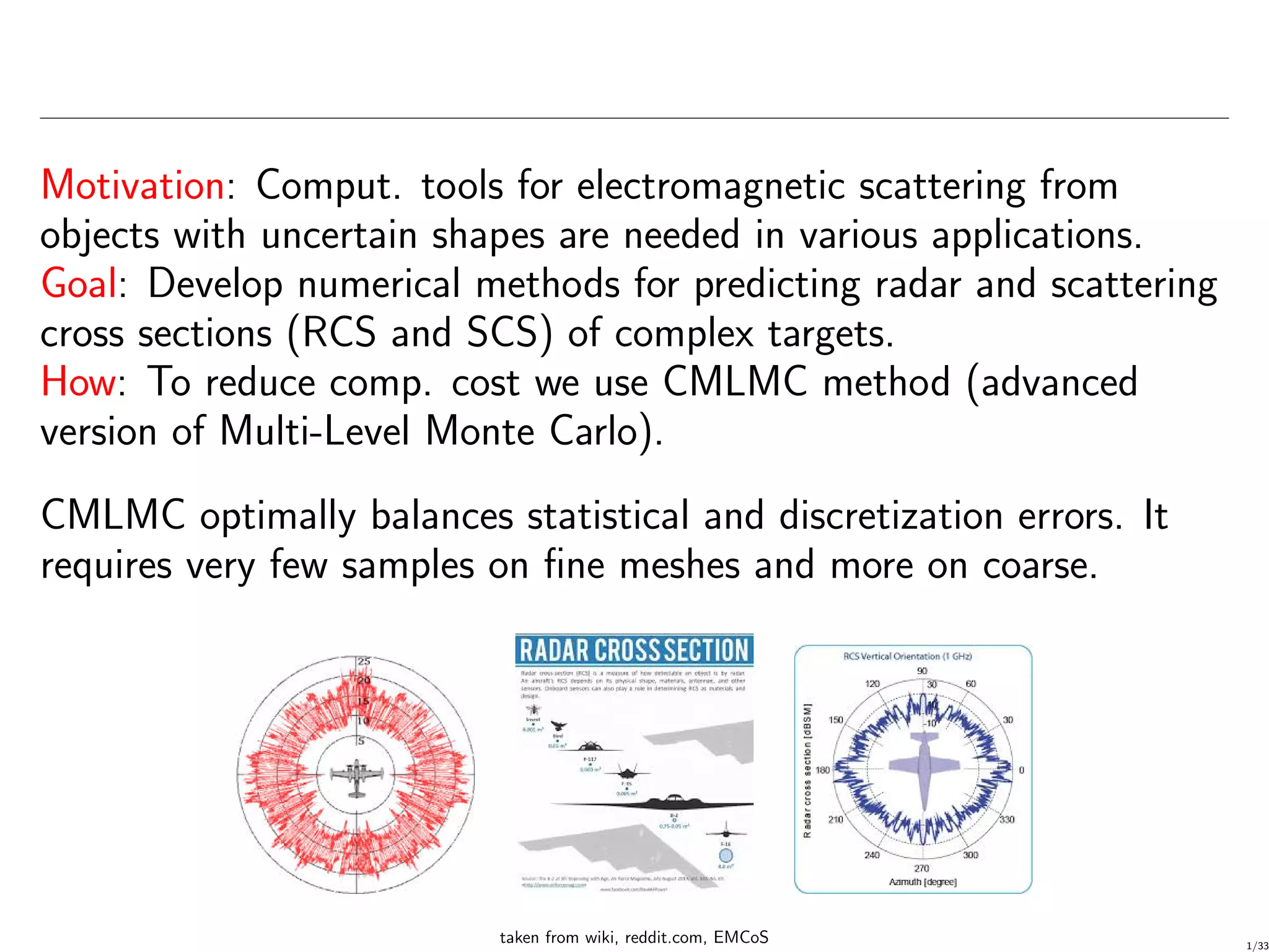
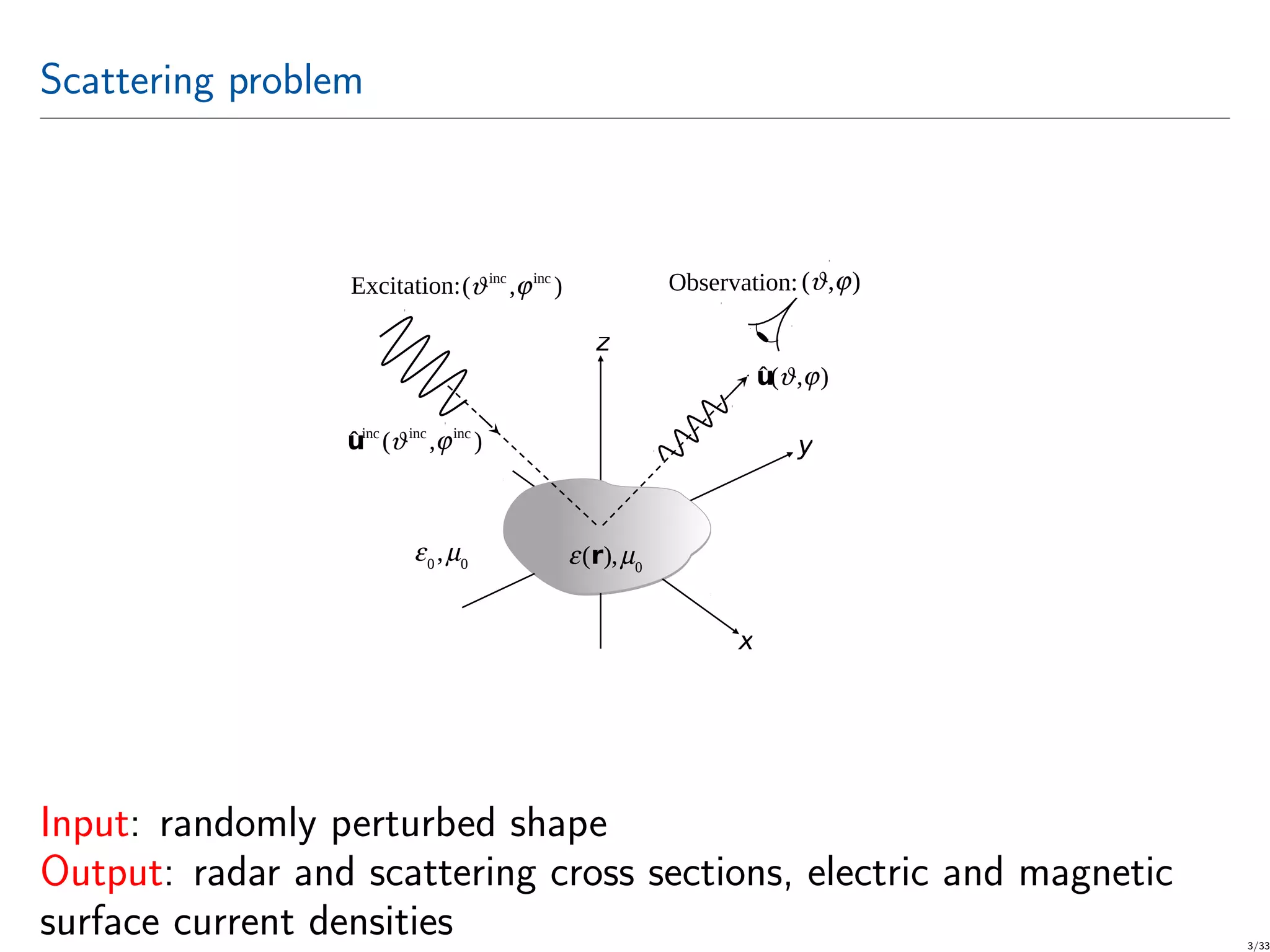
The document discusses the development of numerical methods for predicting electromagnetic scattering from dielectric objects of uncertain shapes using a computational approach called continuation multilevel Monte Carlo (CMLMC). This method optimizes the balance between statistical and discretization errors, demonstrating significant computational efficiency compared to traditional Monte Carlo methods. Through various numerical tests and methodologies outlined, the authors show that their CMLMC approach can achieve faster and more accurate results in electromagnetic wave scattering analysis.
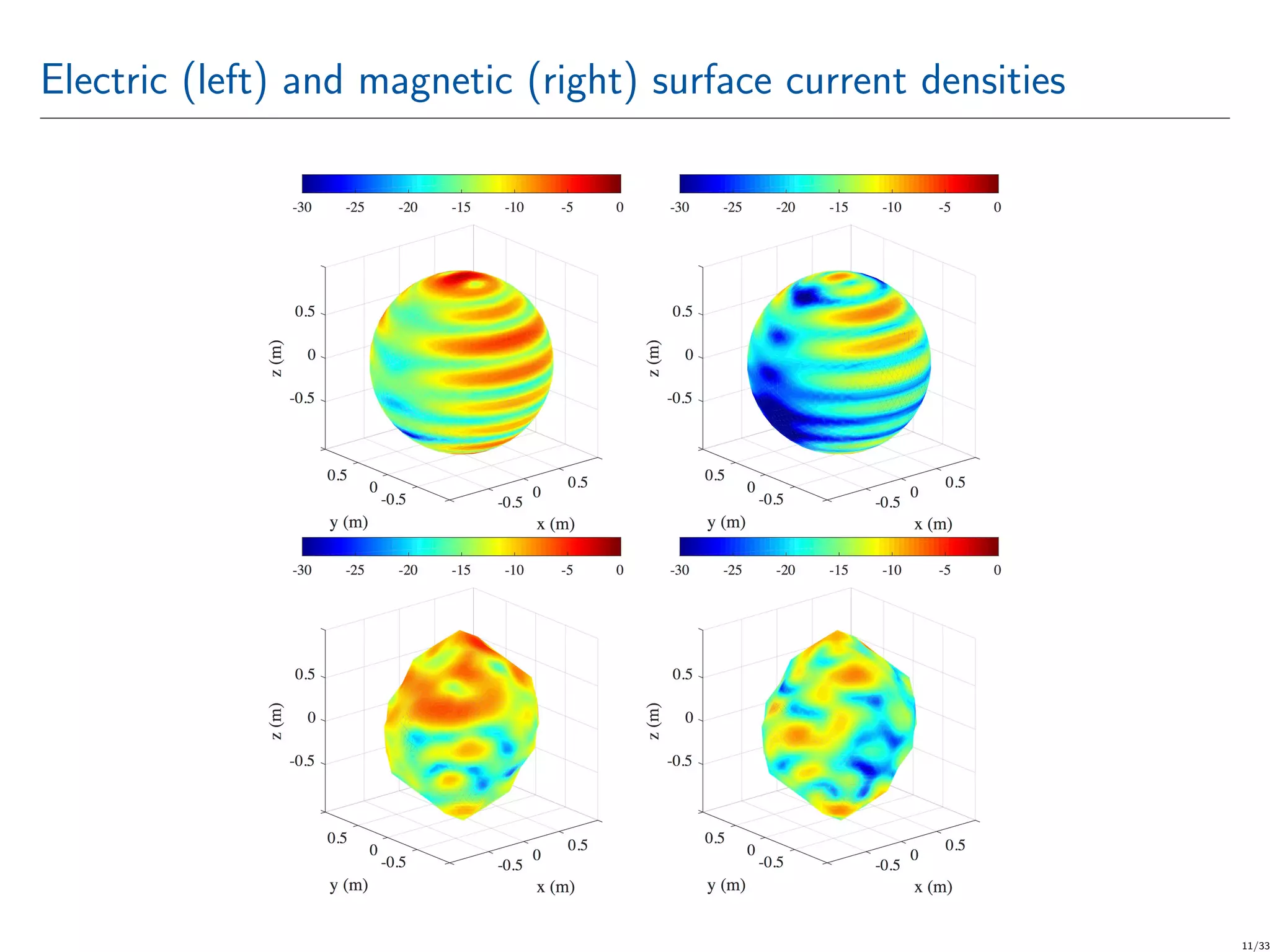
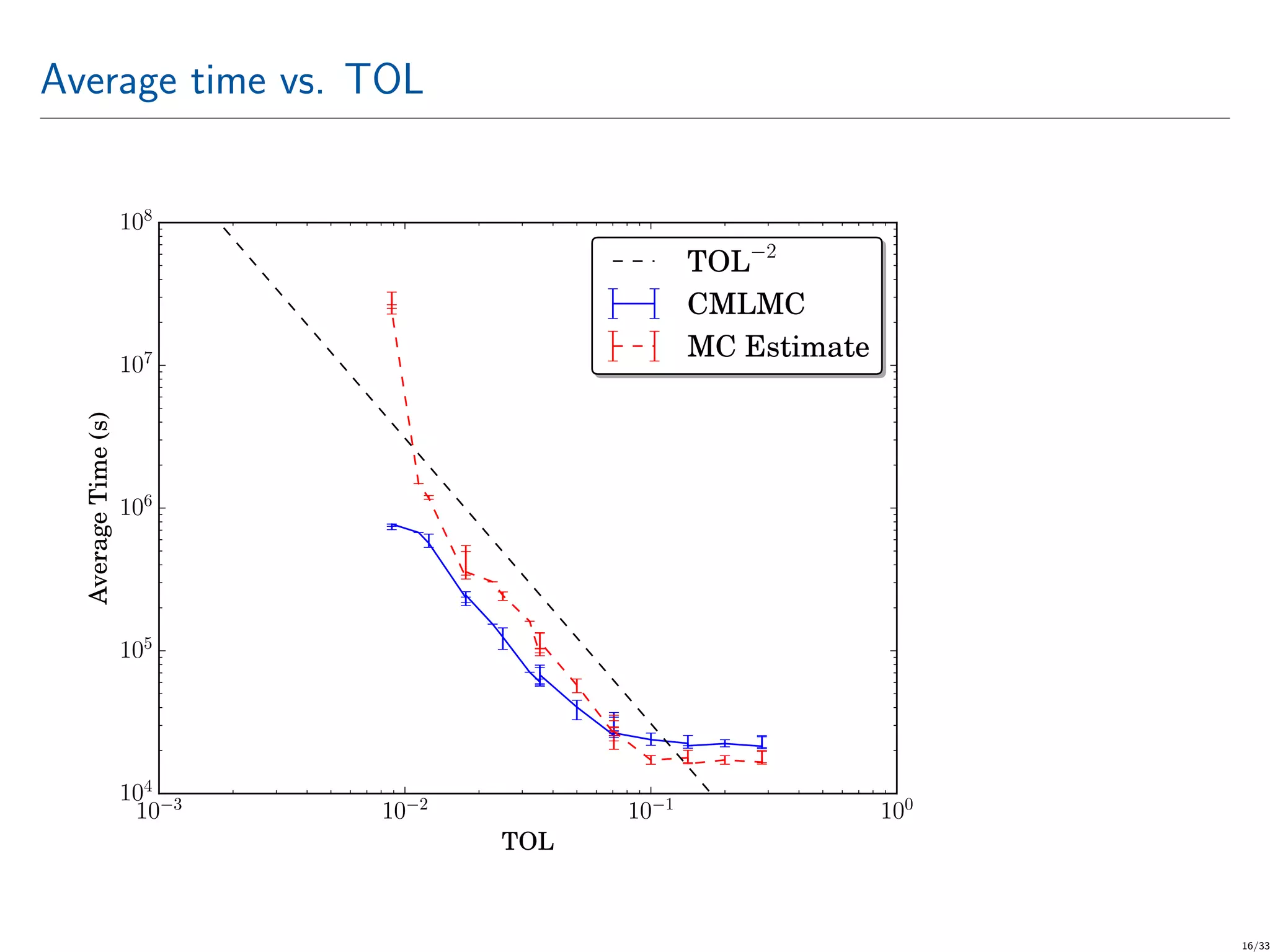
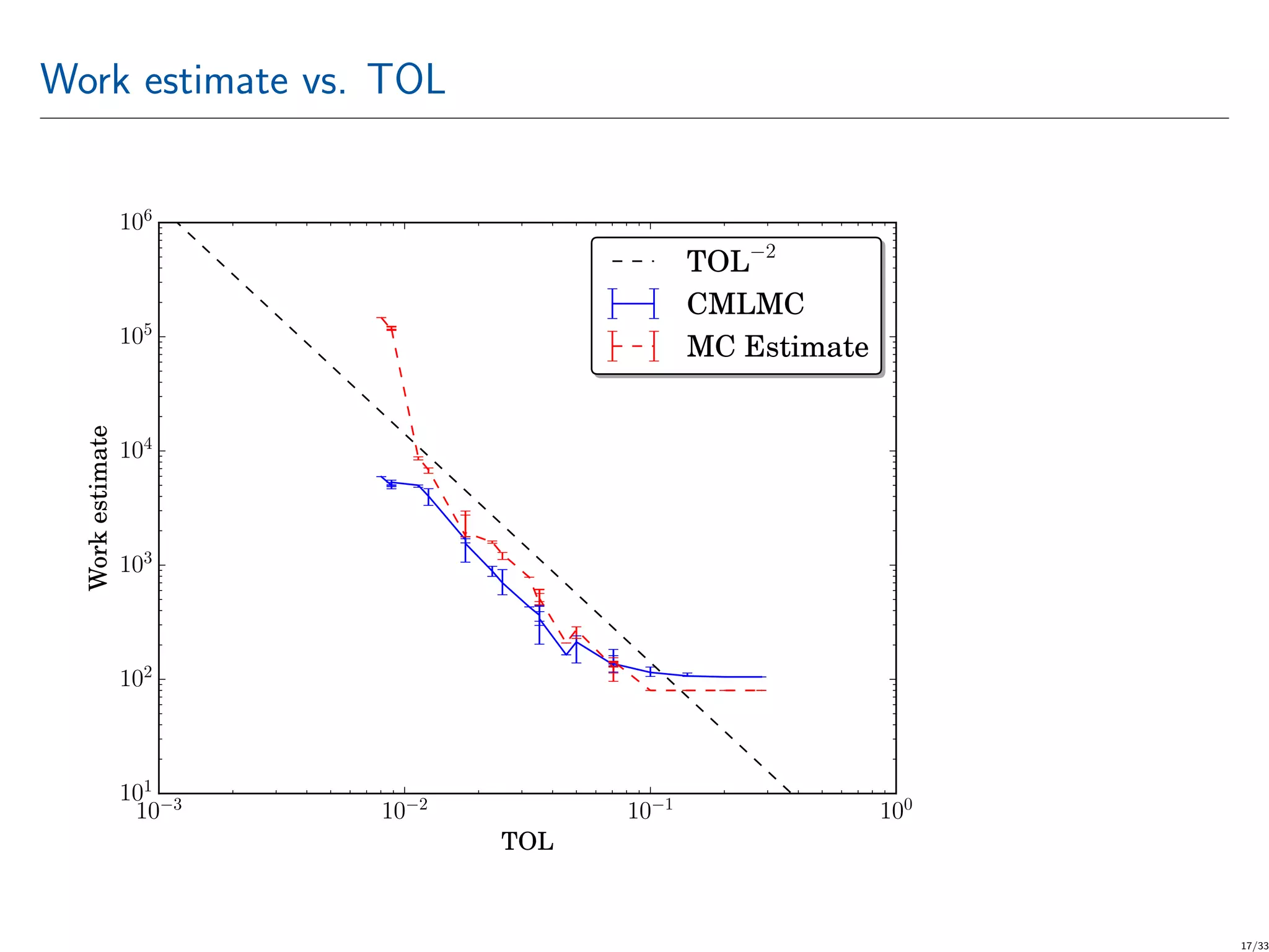
![CMLMC numerical tests The QoI is the SCS over a user-defined solid angle Ω = [1/6, 11/36]π rad × [5/12, 19/36]π rad (i.e., a measure of far-field scattered power in a cone). RVs are: a1, a2 ∼ U[−0.14, 0.14] m, ϕx, ϕy, ϕz ∼ U[0.2, 3] rad, lx, ly, lz ∼ U[0.9, 1.1]; U[a, b] is the uniform distribution between a and b. CMLMC runs for TOL ranging from 0.2 to 0.008. At TOL ≈ 0.008, CMLMC requires L = 5 meshes with {320, 1280, 5120, 20480, 81920} triangles. 15/33](https://image.slidesharecdn.com/computationofelectromagneticfieldsscatteredfromdielectricobjectsofuncertainshapesusingmlmc-200306133636/75/Computation-of-electromagnetic-fields-scattered-from-dielectric-objects-of-uncertain-shapes-using-MLMC-algorithm-16-2048.jpg)
![V = Var[G ] vs. (strong convergence) 0 1 2 3 4 10−7 10−6 10−5 10−4 10−3 10−2 10−1 V 2−5 G assumed strong convergence curve 2−5 (q2 = 5). 20/33](https://image.slidesharecdn.com/computationofelectromagneticfieldsscatteredfromdielectricobjectsofuncertainshapesusingmlmc-200306133636/75/Computation-of-electromagnetic-fields-scattered-from-dielectric-objects-of-uncertain-shapes-using-MLMC-algorithm-21-2048.jpg)
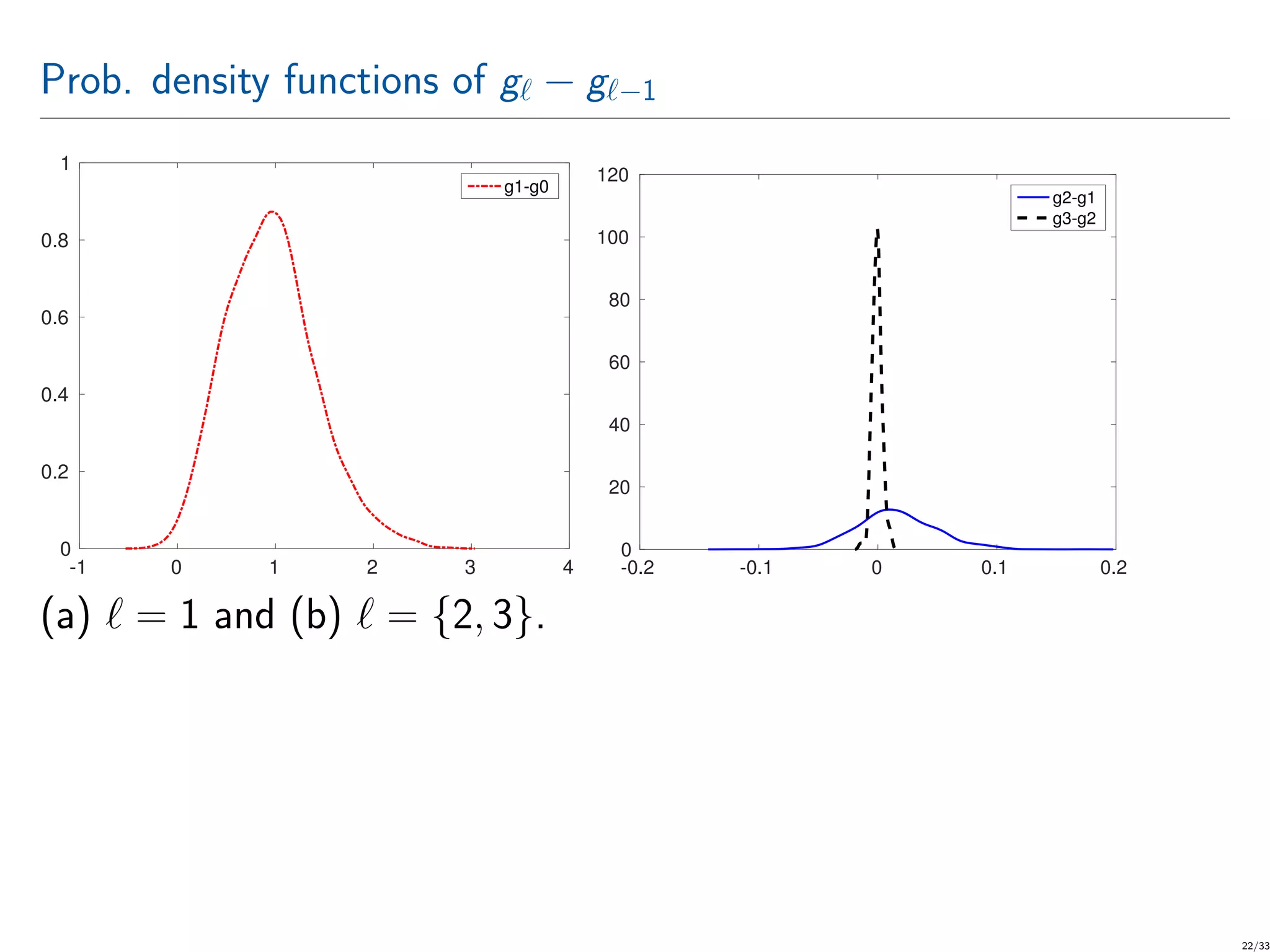
![CMLMC repeating Let {P }L =0 be sequences of meshes with h = h0β− , β > 1. Let g (ξ) represent the approximation to g(ξ) computed using mesh P . E[gL] = L =0 E[G ] (4) where G is defined as G = g0 if = 0 g − g −1 if > 0 . (5) Note that g and g −1 are computed using the same input random parameter ξ. 28/33](https://image.slidesharecdn.com/computationofelectromagneticfieldsscatteredfromdielectricobjectsofuncertainshapesusingmlmc-200306133636/75/Computation-of-electromagnetic-fields-scattered-from-dielectric-objects-of-uncertain-shapes-using-MLMC-algorithm-29-2048.jpg)
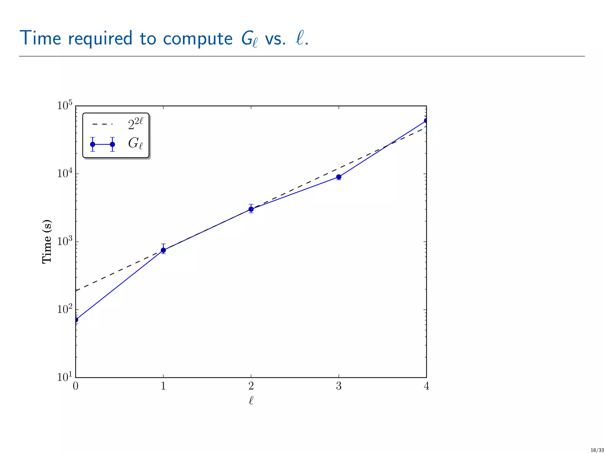
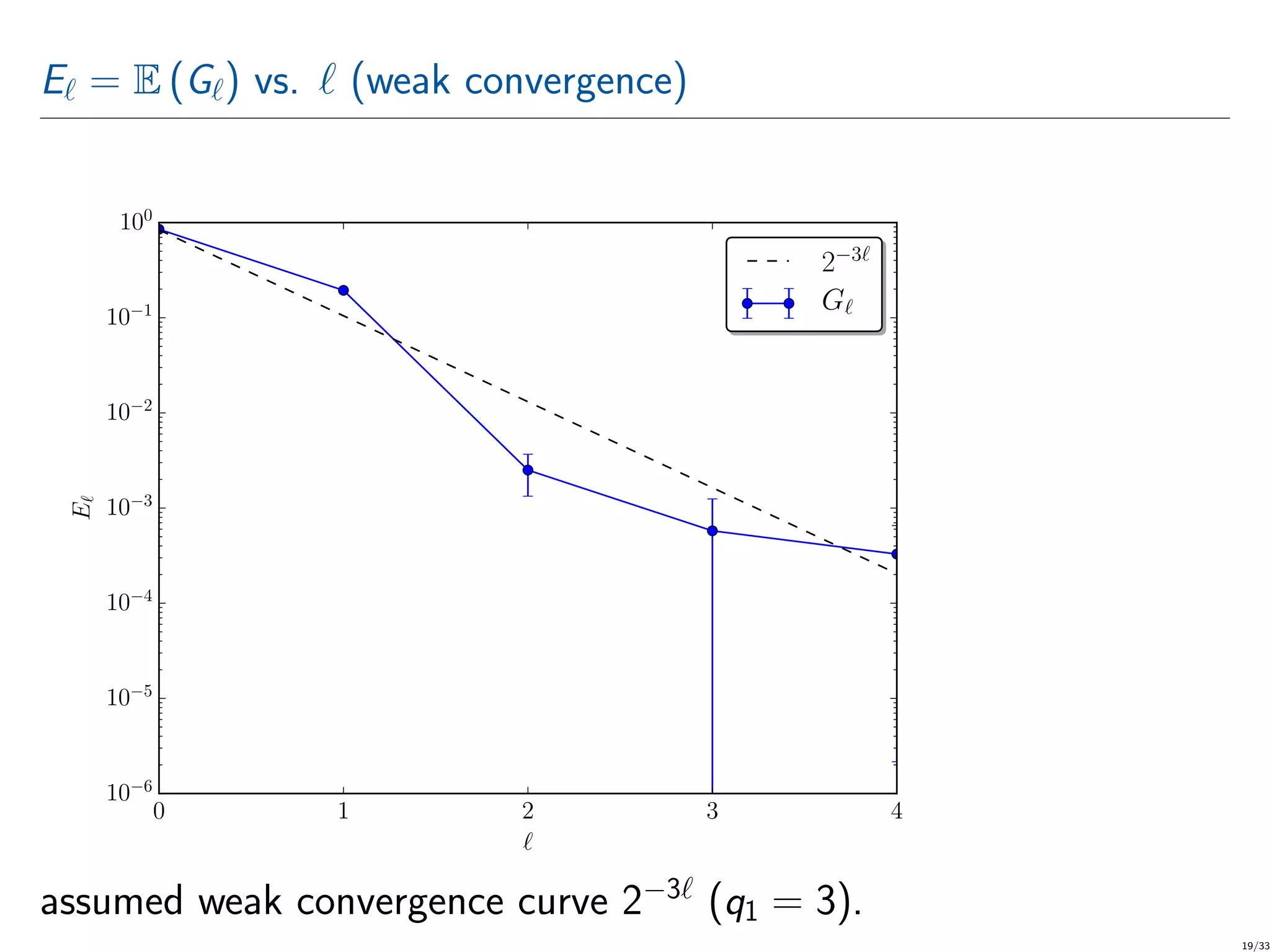
![CMLMC repeating E[G ] ≈ ∼ G = M−1 M m=1 G ,m, E[g − g ] ≈ QW hq1 (6a) Var[g − g −1] ≈ QShq2 −1 (6b) for QW = 0, QS > 0, q1 > 0, and 0 < q2 ≤ 2q1. QoI A = L =0 ∼ G . Let the average cost of generating one sample of G (cost of one deterministic simulation for one random realization) be W ∝ h−dγ = h−dγ 0 β dγ (7) 29/33](https://image.slidesharecdn.com/computationofelectromagneticfieldsscatteredfromdielectricobjectsofuncertainshapesusingmlmc-200306133636/75/Computation-of-electromagnetic-fields-scattered-from-dielectric-objects-of-uncertain-shapes-using-MLMC-algorithm-30-2048.jpg)
![CMLMC repeating The total CMLMC computational cost is W = L =0 M W . (8) The estimator A satisfies a tolerance with a prescribed failure probability 0 < ν ≤ 1, i.e., P[|E[g] − A| ≤ TOL] ≥ 1 − ν (9) while minimizing W . The total error is split into bias and statistical error, |E[g] − A| ≤ |E[g − A]| Bias + |E[A] − A| Statistical error 30/33](https://image.slidesharecdn.com/computationofelectromagneticfieldsscatteredfromdielectricobjectsofuncertainshapesusingmlmc-200306133636/75/Computation-of-electromagnetic-fields-scattered-from-dielectric-objects-of-uncertain-shapes-using-MLMC-algorithm-31-2048.jpg)
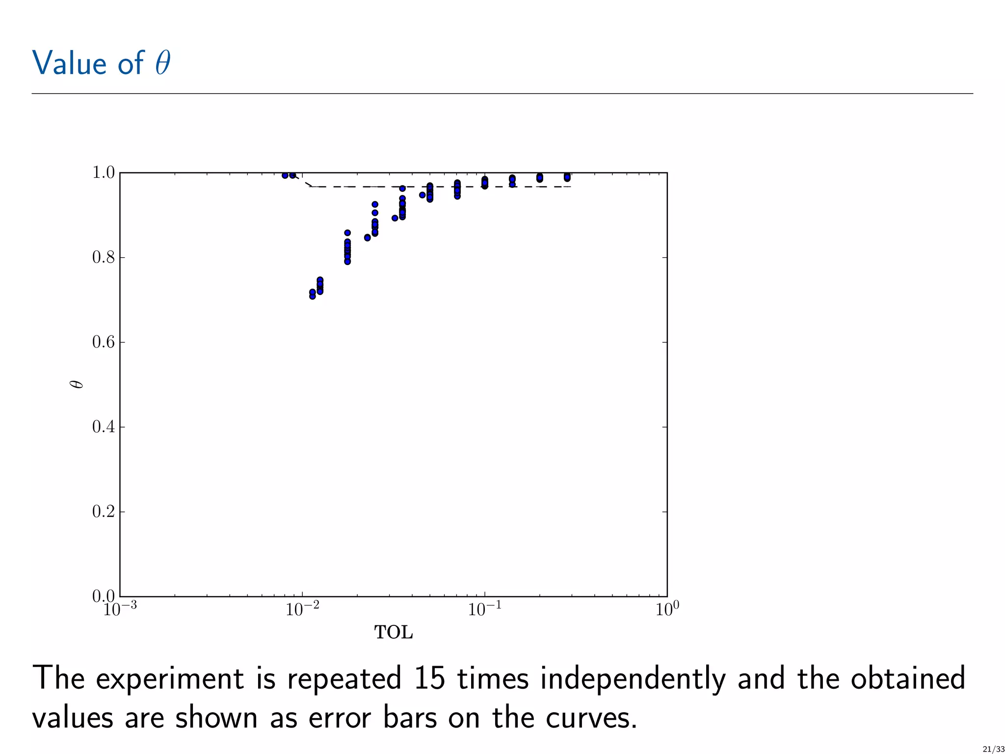
![CMLMC repeating Let θ ∈ (0, 1) be a splitting parameter, so that TOL = (1 − θ)TOL Bias tolerance + θTOL Statistical error tolerance . (10) The CMLMC algorithm bounds the bias, B = |E[g − A]|, and the statistical error as B = |E[g − A]| ≤ (1 − θ)TOL (11) |E[A] − A| ≤ θTOL (12) where the latter bound holds with probability 1 − ν. To satisfy condition in (12) we require: Var[A] ≤ θTOL Cν 2 (13) for some given confidence parameter, Cν, such that Φ(Cν) = 1 − ν 2, Φ is the cdf of a standard normal random variable. 31/33](https://image.slidesharecdn.com/computationofelectromagneticfieldsscatteredfromdielectricobjectsofuncertainshapesusingmlmc-200306133636/75/Computation-of-electromagnetic-fields-scattered-from-dielectric-objects-of-uncertain-shapes-using-MLMC-algorithm-32-2048.jpg)
![CMLMC repeating By construction of the MLMC estimator, E[A] = E[gL], and by independence, Var[A] = L =0 V M−1 , where V = Var[G ]. Given L, TOL, and 0 < θ < 1, and by minimizing W subject to the statistical constraint (13) for {M }L =0 gives the following optimal number of samples per level (apply ceiling function to M if necessary): M = Cν θTOL 2 V W L =0 V W . (14) Summing the optimal numbers of samples over all levels yields the following expression for the total optimal computational cost in terms of TOL: W (TOL, L) = Cν θTOL 2 L =0 V W 2 . (15) 32/33](https://image.slidesharecdn.com/computationofelectromagneticfieldsscatteredfromdielectricobjectsofuncertainshapesusingmlmc-200306133636/75/Computation-of-electromagnetic-fields-scattered-from-dielectric-objects-of-uncertain-shapes-using-MLMC-algorithm-33-2048.jpg)