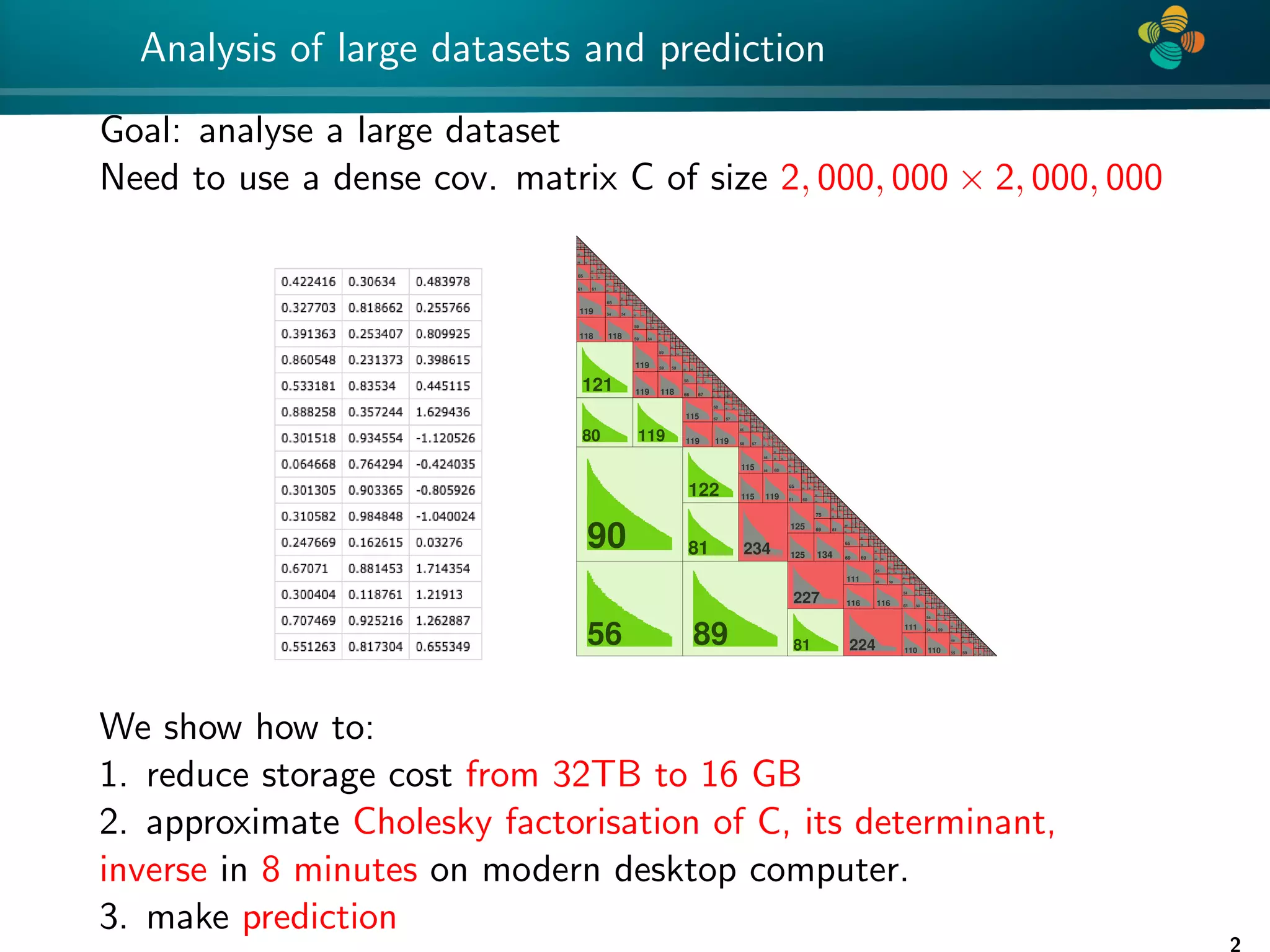
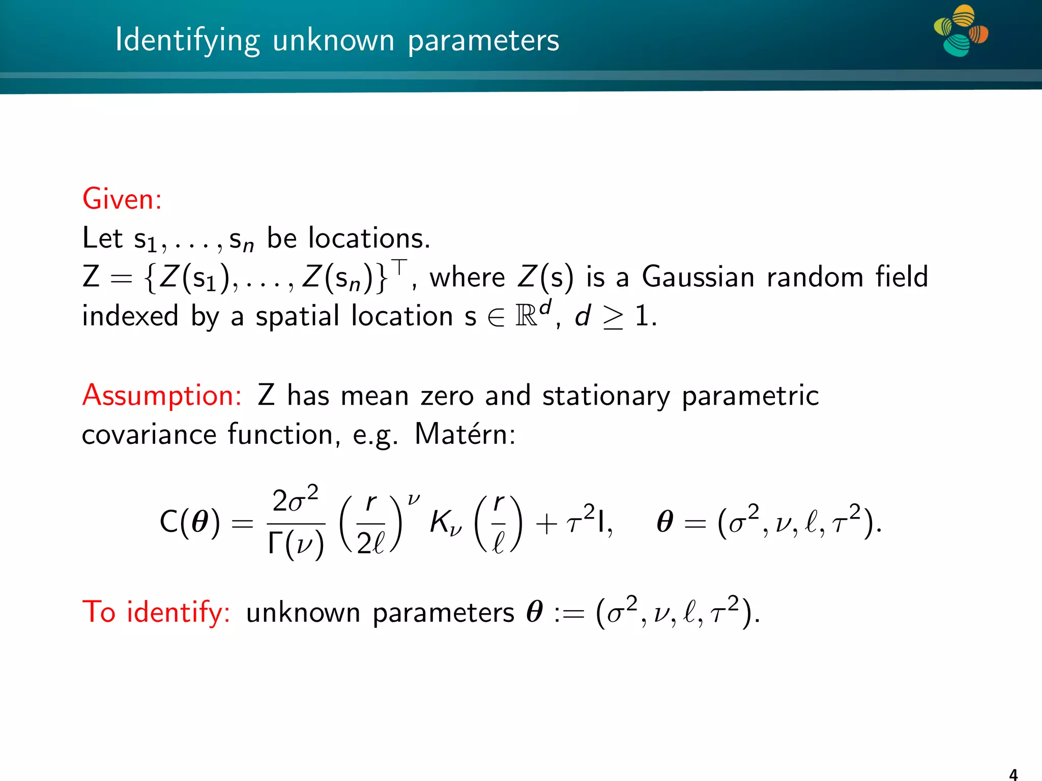
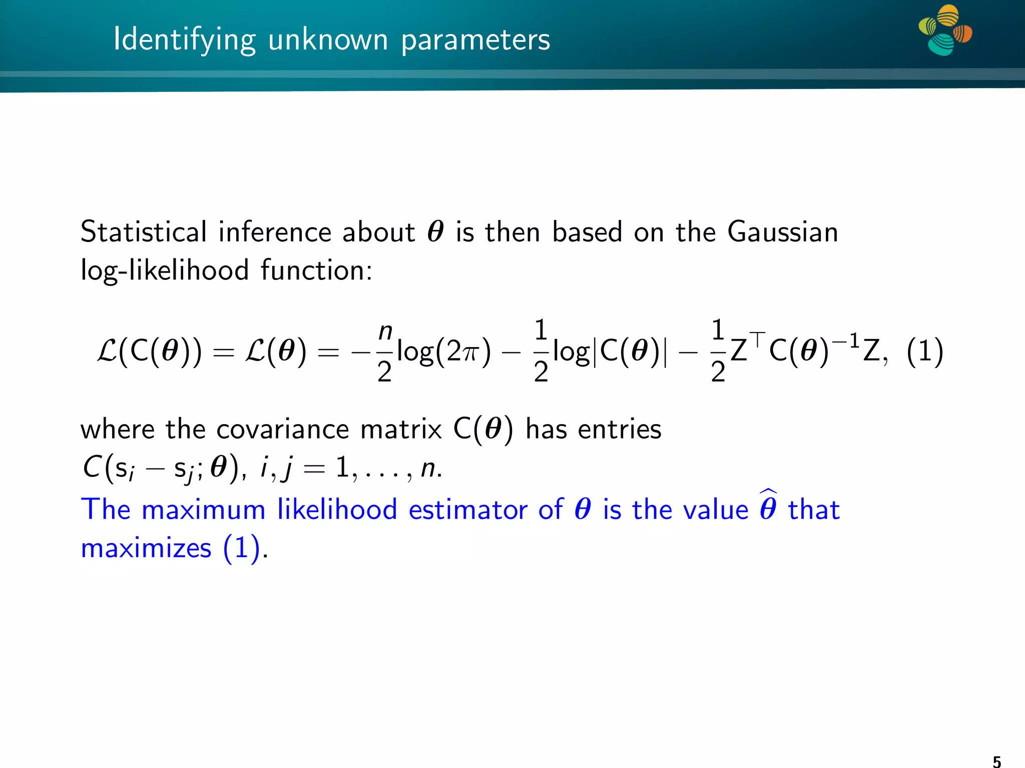
The document presents a method for identifying unknown parameters and making predictions using hierarchical matrices, highlighting a case study of reducing storage costs for a large covariance matrix. It demonstrates the maximum likelihood estimation of parameters through Gaussian log-likelihood functions and evaluates the effectiveness of this method in comparison to traditional machine learning approaches. The document also outlines the tools, error analysis, and structure of the discussion to improve statistical models and data analysis.
![4 * The structure of the talk 1. Motivation: improve statistical models, data analysis, prediction 2. Identification of unknown parameters via maximizing Gaussian log-likelihood (MLE) 3. Tools: Hierarchical matrices [Hackbusch 1999] 4. Matérn covariance function, joint Gaussian log-likelihood 5. Error analysis 6. Prediction at new locations 7. Comparison with machine learning methods 3](https://image.slidesharecdn.com/talklitvinenkouncecomp21-210628075644/75/Identification-of-unknown-parameters-and-prediction-with-hierarchical-matrices-Comparison-with-ML-methods-3-2048.jpg)
![4 * What will change after H-matrix approximation? Approximate C by CH 1. How the eigenvalues of C and CH differ ? 2. How det(C) differs from det(CH) ? 3. How L differs from LH ? [Mario Bebendorf et al] 4. How C−1 differs from (CH)−1 ? [Mario Bebendorf et al] 5. How L̃(θ, k) differs from L(θ)? 6. What is optimal H-matrix rank? 7. How θH differs from θ? For theory, estimates for the rank and accuracy see works of Bebendorf, Grasedyck, Le Borne, Hackbusch,... 7](https://image.slidesharecdn.com/talklitvinenkouncecomp21-210628075644/75/Identification-of-unknown-parameters-and-prediction-with-hierarchical-matrices-Comparison-with-ML-methods-7-2048.jpg)
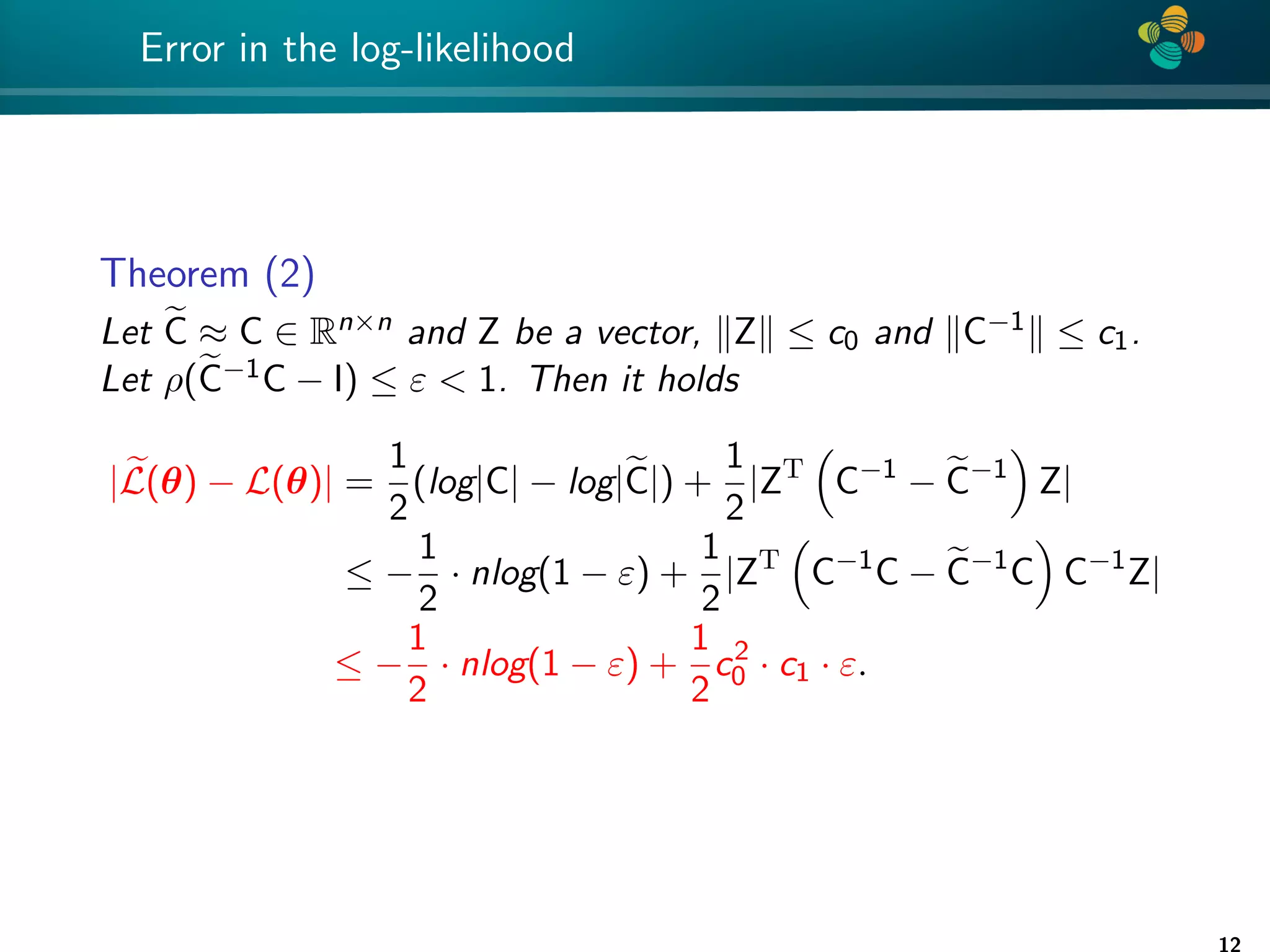
![4 * Error analysis Theorem (1) Let e C be an H-matrix approximation of matrix C ∈ Rn×n such that ρ(e C−1 C − I) ≤ ε 1. Then |log det C − log det e C| ≤ −nlog(1 − ε), (3) Proof: See [Ballani, Kressner 14] and [Ipsen 05]. Remark: factor n is pessimistic and is not really observed numerically. 11](https://image.slidesharecdn.com/talklitvinenkouncecomp21-210628075644/75/Identification-of-unknown-parameters-and-prediction-with-hierarchical-matrices-Comparison-with-ML-methods-11-2048.jpg)
![4 * Error convergence 0 10 20 30 40 50 60 70 80 90 100 −25 −20 −15 −10 −5 0 rank k log(rel. error) Spectral norm, L=0.1, nu=1 Frob. norm, L=0.1 Spectral norm, L=0.2 Frob. norm, L=0.2 Spectral norm, L=0.5 Frob. norm, L=0.5 0 10 20 30 40 50 60 70 80 90 100 −16 −14 −12 −10 −8 −6 −4 −2 0 rank k log(rel. error) Spectral norm, L=0.1, nu=0.5 Frob. norm, L=0.1 Spectral norm, L=0.2 Frob. norm, L=0.2 Spectral norm, L=0.5 Frob. norm, L=0.5 Convergence of the H-matrix approximation errors for covariance lengths {0.1, 0.2, 0.5}; (left) ν = 1 and (right) ν = 0.5, computational domain [0, 1]2. 16](https://image.slidesharecdn.com/talklitvinenkouncecomp21-210628075644/75/Identification-of-unknown-parameters-and-prediction-with-hierarchical-matrices-Comparison-with-ML-methods-16-2048.jpg)