Downloaded 13 times

![Challenge: Data Representation Java objects often many times larger than data class User(name: String, friends: Array[Int]) User(“Bobby”, Array(1, 2)) User 0x… 0x… String 3 0 1 2 Bobby 5 0x… int[] char[] 5](https://image.slidesharecdn.com/bigdata-part-two-161207131918/75/Bigdata-processing-with-Spark-part-II-45-2048.jpg)
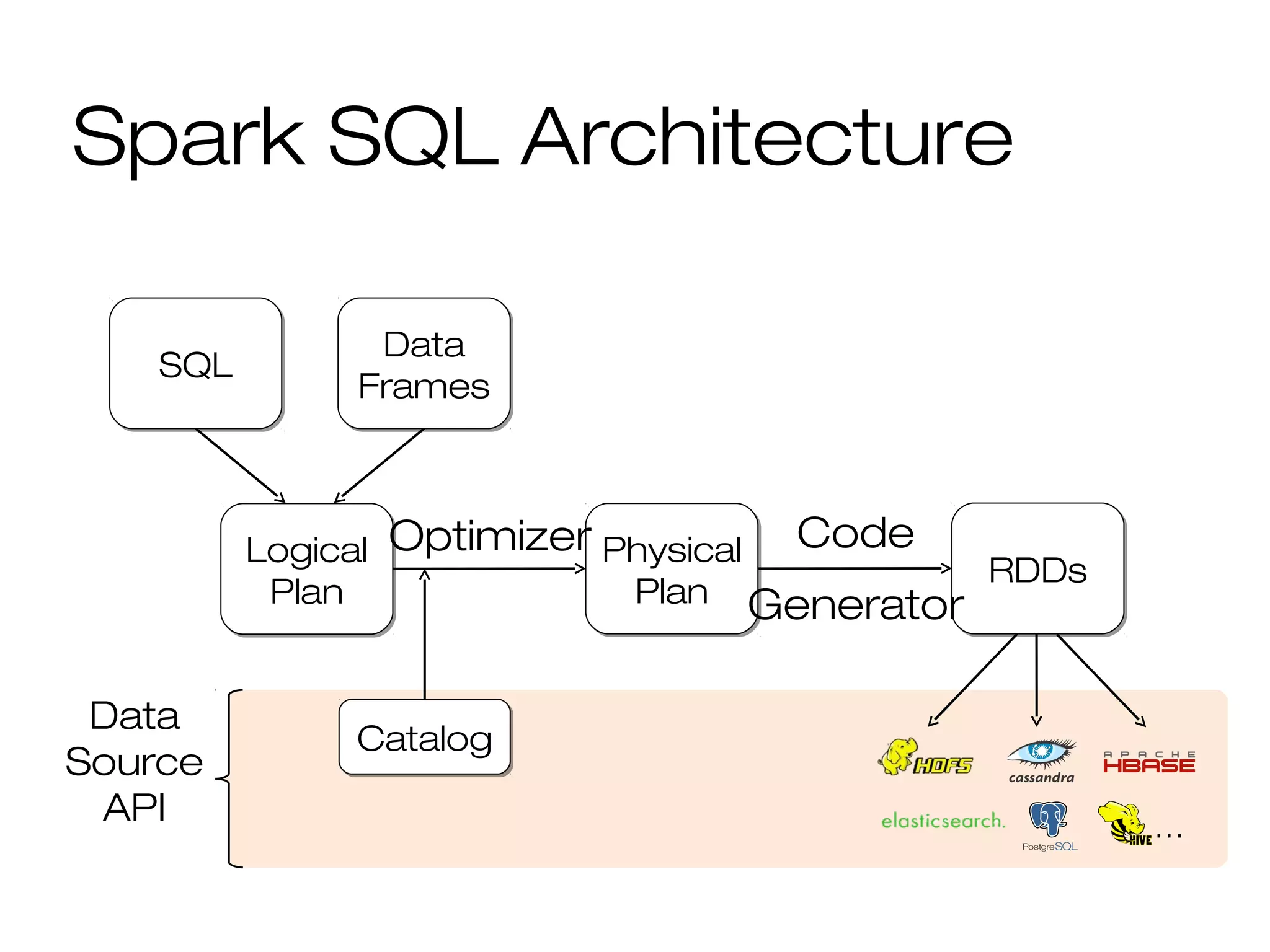
![DataFrame API DataFrames hold rows with a known schema and offer relational operations through a DSL c = HiveContext() users = c.sql(“select * from users”) ma_users = users[users.state == “MA”] ma_users.count() ma_users.groupBy(“name”).avg(“age”) ma_users.map(lambda row: row.user.toUpper()) Expression AST](https://image.slidesharecdn.com/bigdata-part-two-161207131918/75/Bigdata-processing-with-Spark-part-II-48-2048.jpg)
![Data Sources Uniform way to access structured data » Apps can migrate across Hive, Cassandra, JSON, … » Rich semantics allows query pushdown into data sources Spark SQL users[users.age > 20] select * from users](https://image.slidesharecdn.com/bigdata-part-two-161207131918/75/Bigdata-processing-with-Spark-part-II-52-2048.jpg)

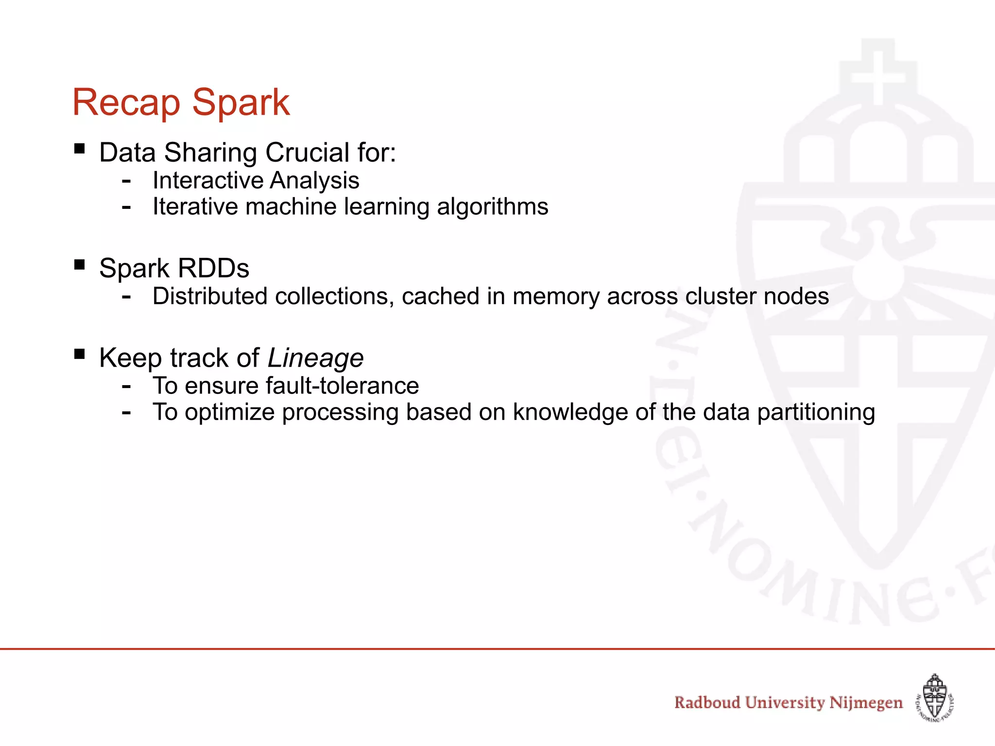
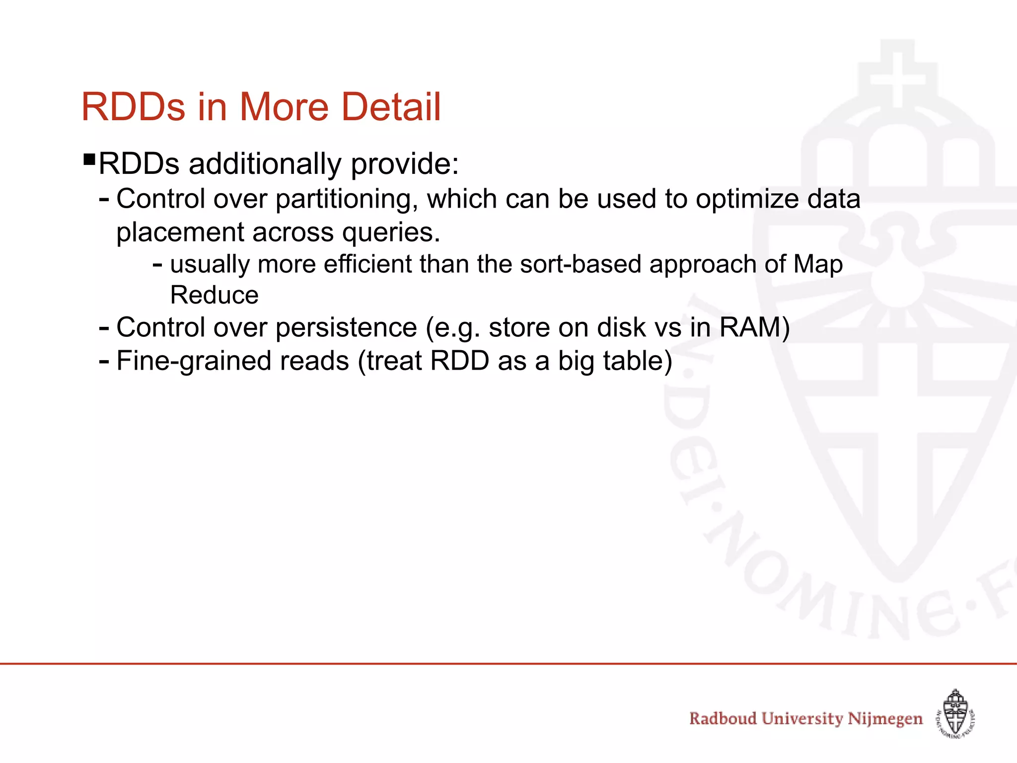
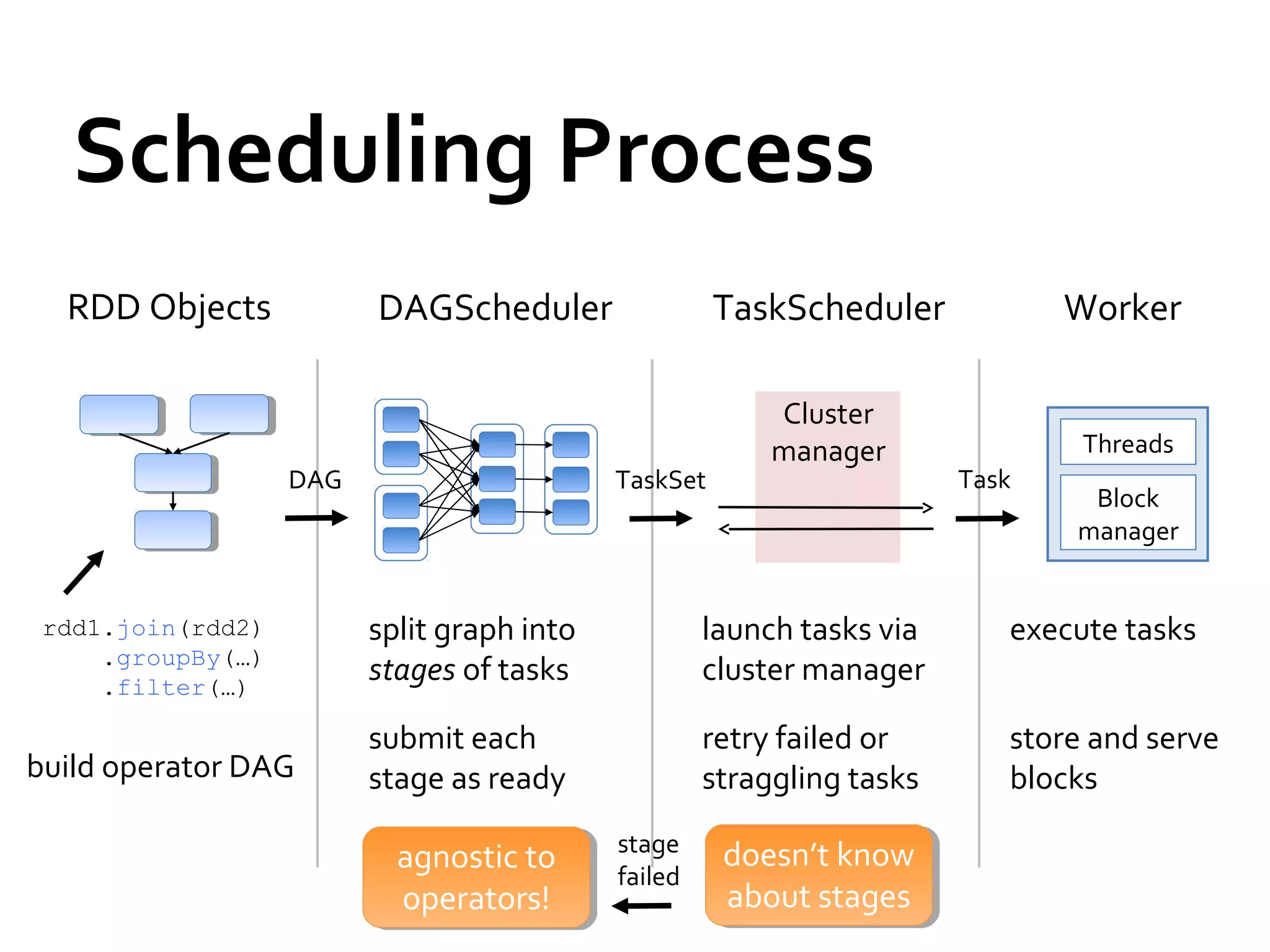
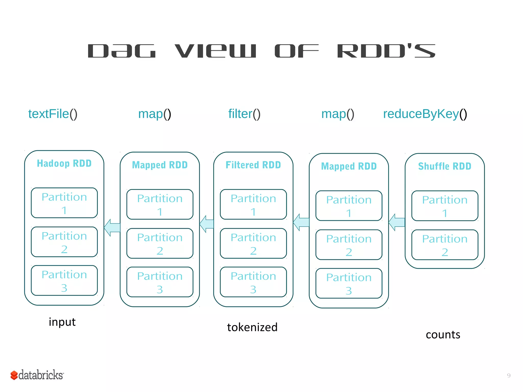
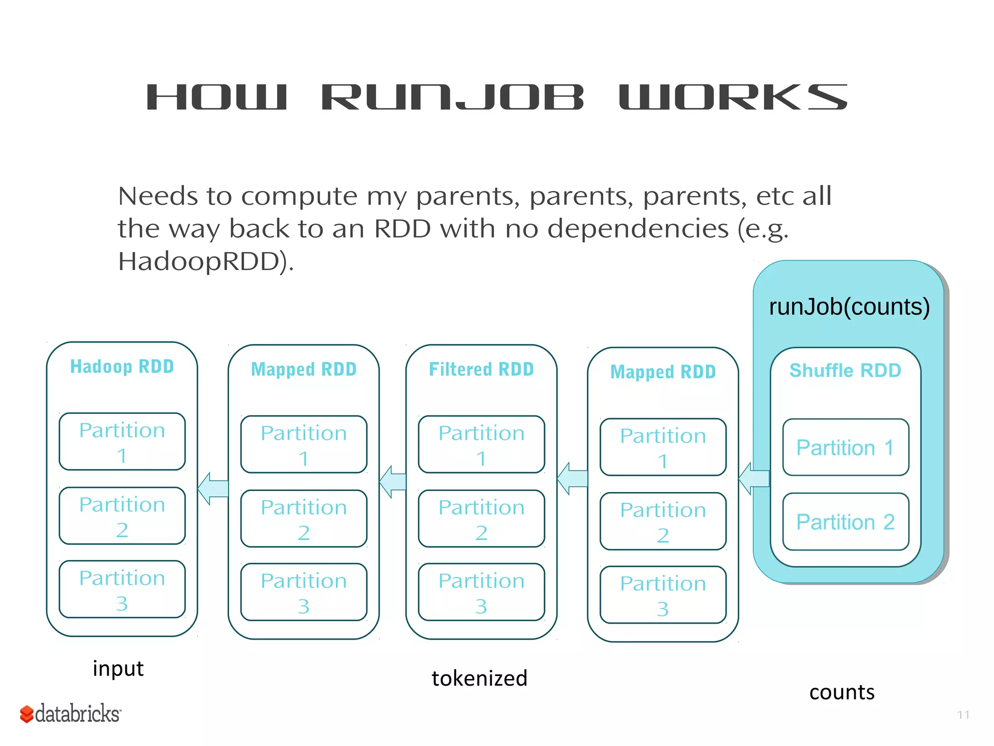
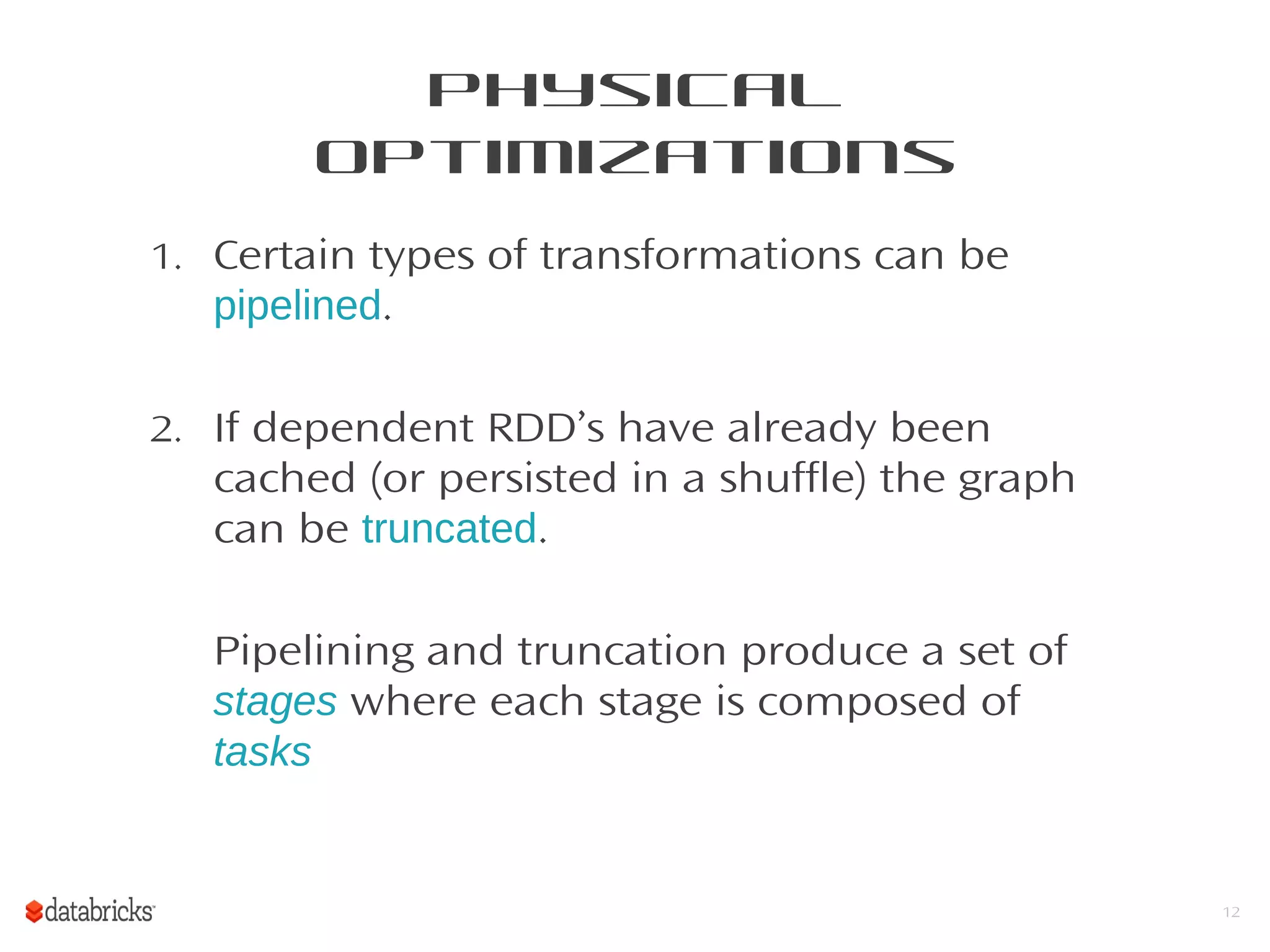
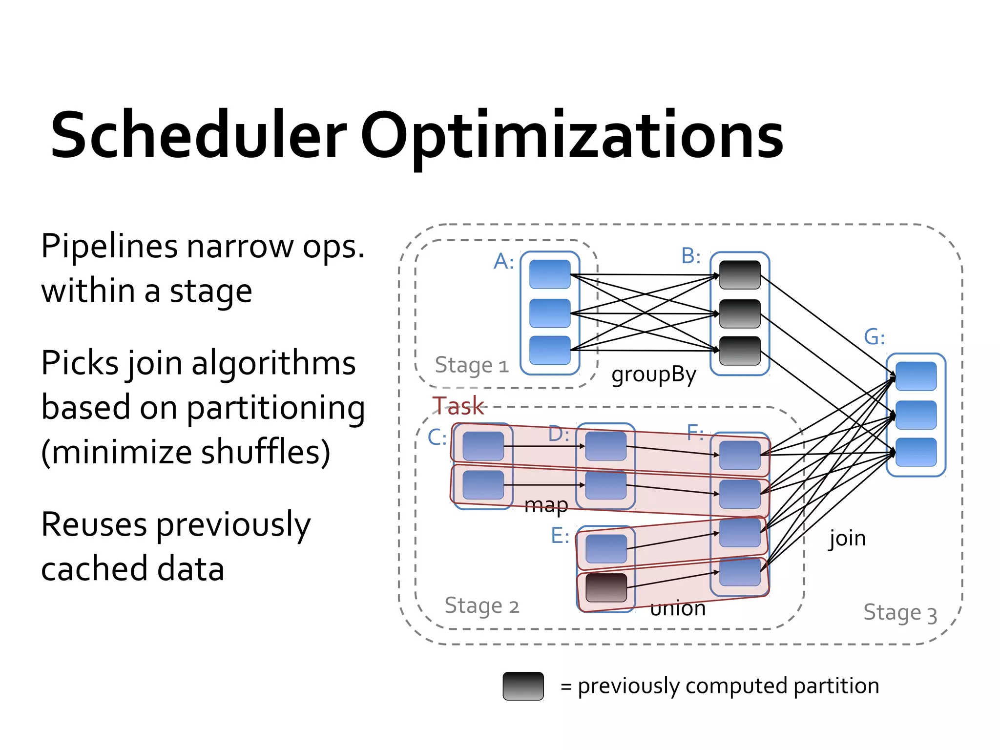
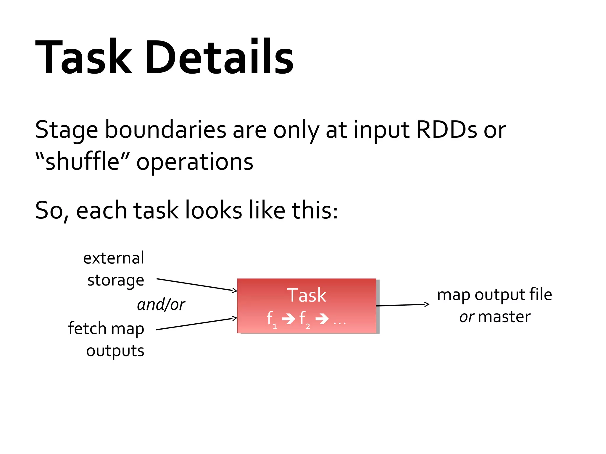
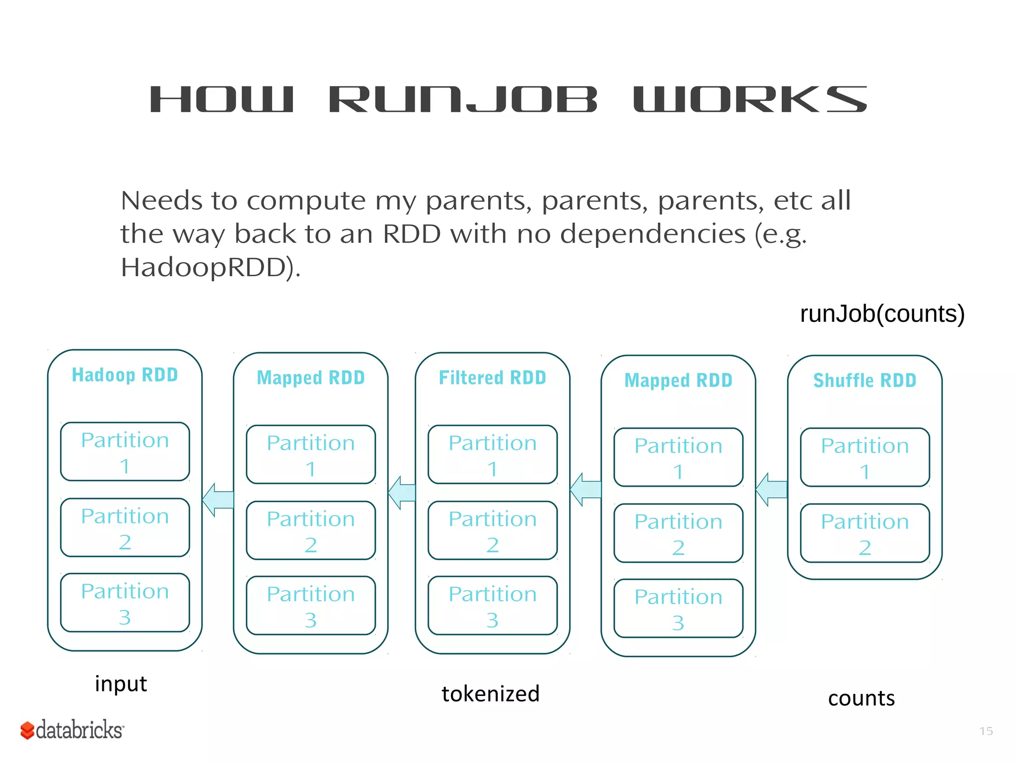
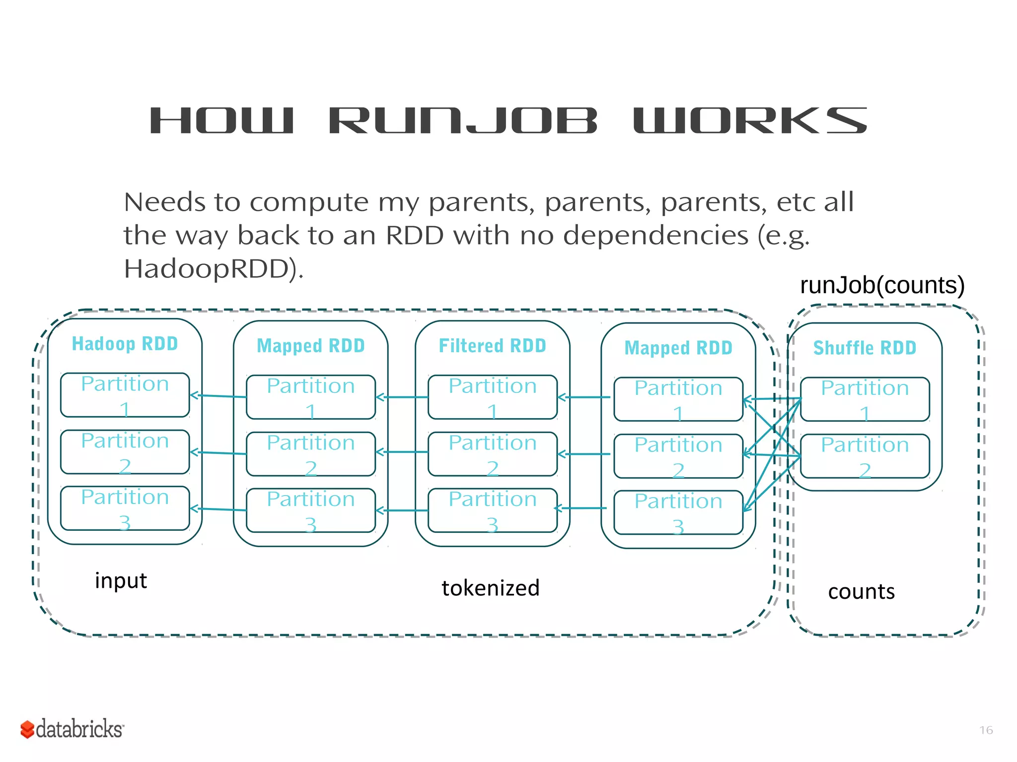
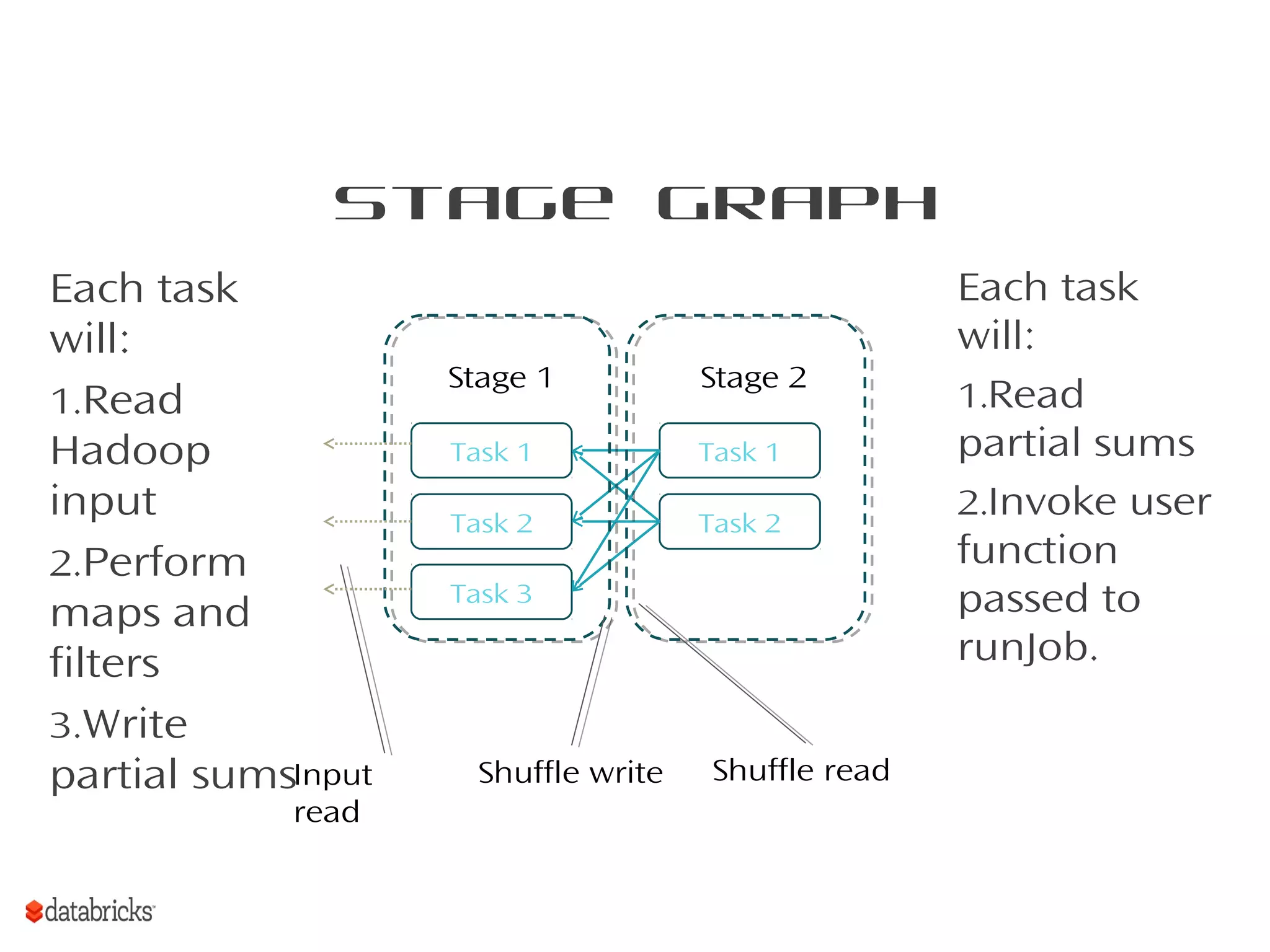
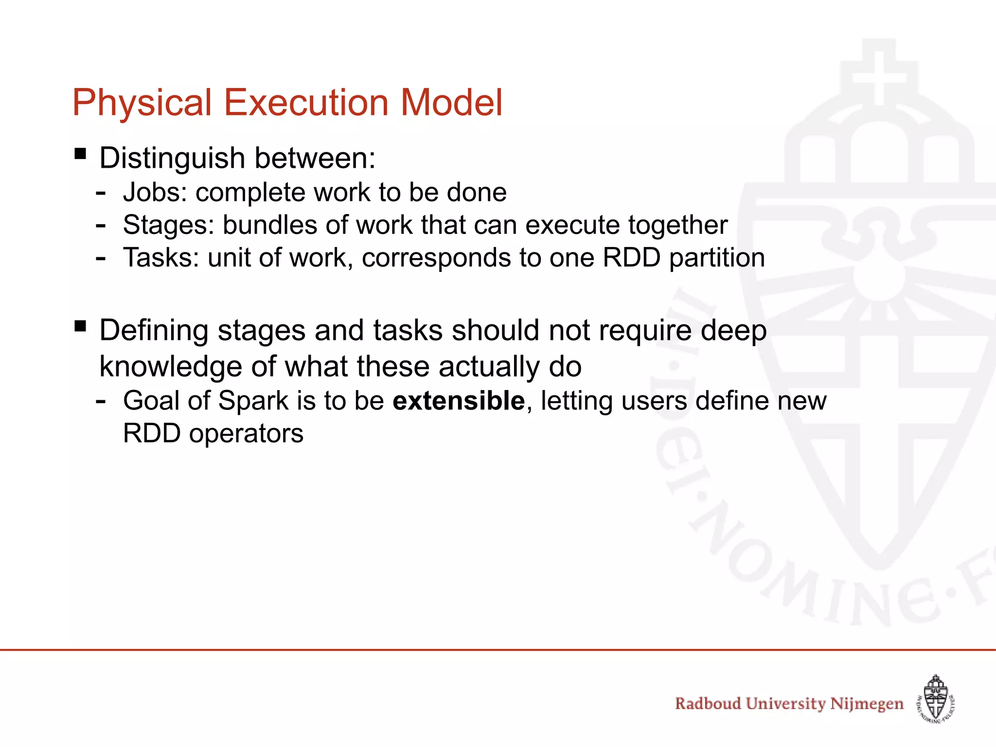
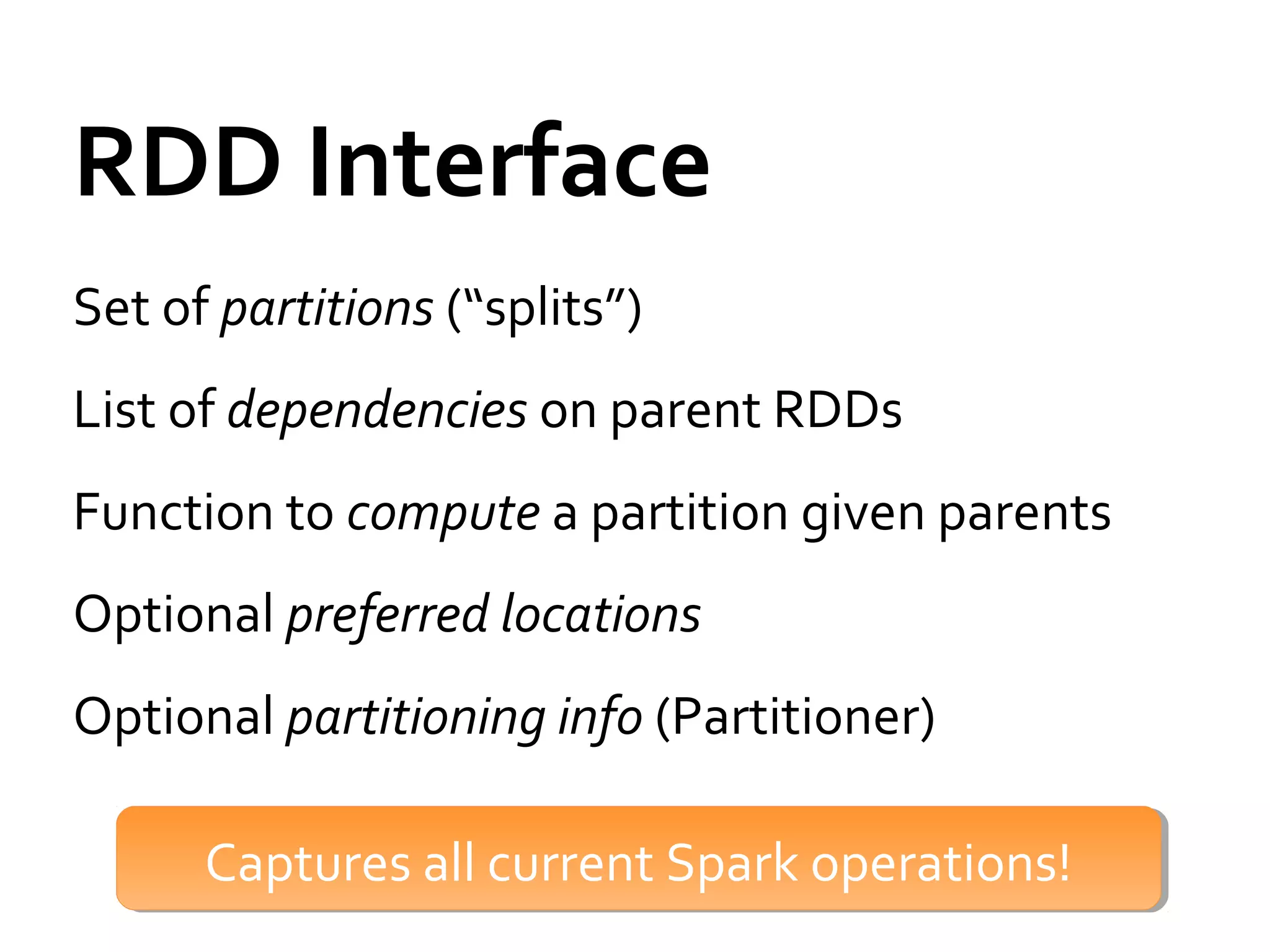
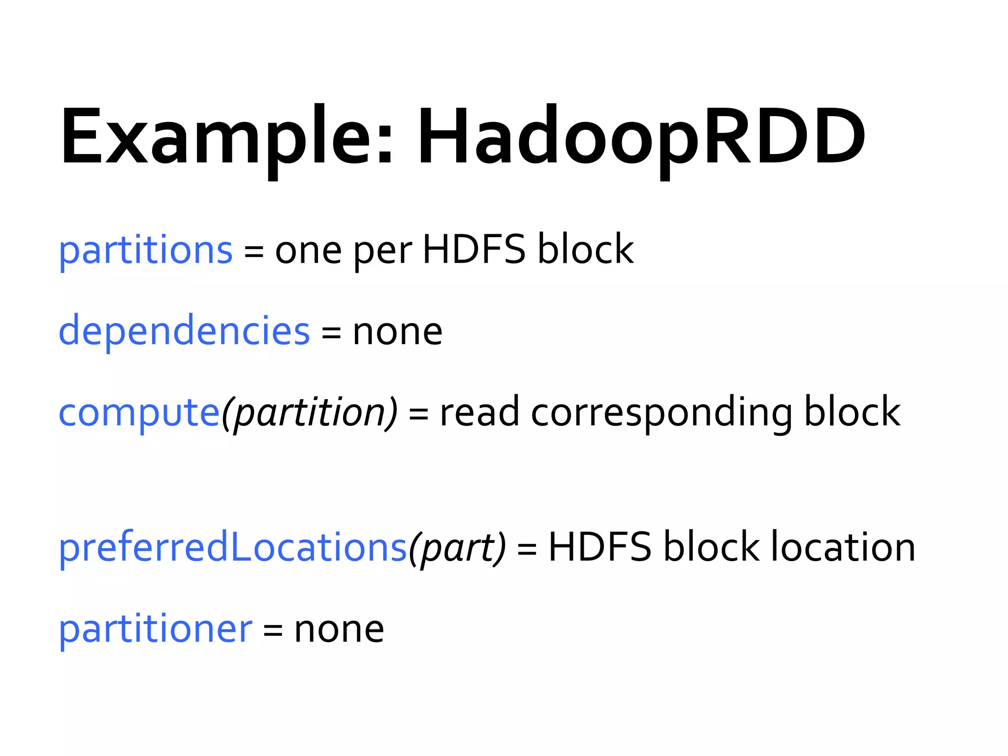
This document provides a summary of Spark RDDs and the Spark execution model: - RDDs (Resilient Distributed Datasets) are Spark's fundamental data structure, representing an immutable distributed collection of objects that can be operated on in parallel. RDDs track lineage to support fault tolerance and optimization. - Spark uses a logical plan built from transformations on RDDs, which is then optimized and scheduled into physical stages and tasks by the Spark scheduler. Tasks operate on partitions of RDDs in a data-parallel manner. - The scheduler pipelines transformations where possible, truncates redundant work, and leverages caching and data locality to improve performance. It splits the graph into stages separated by shuffle operations or parent RDD boundaries