Download to read offline
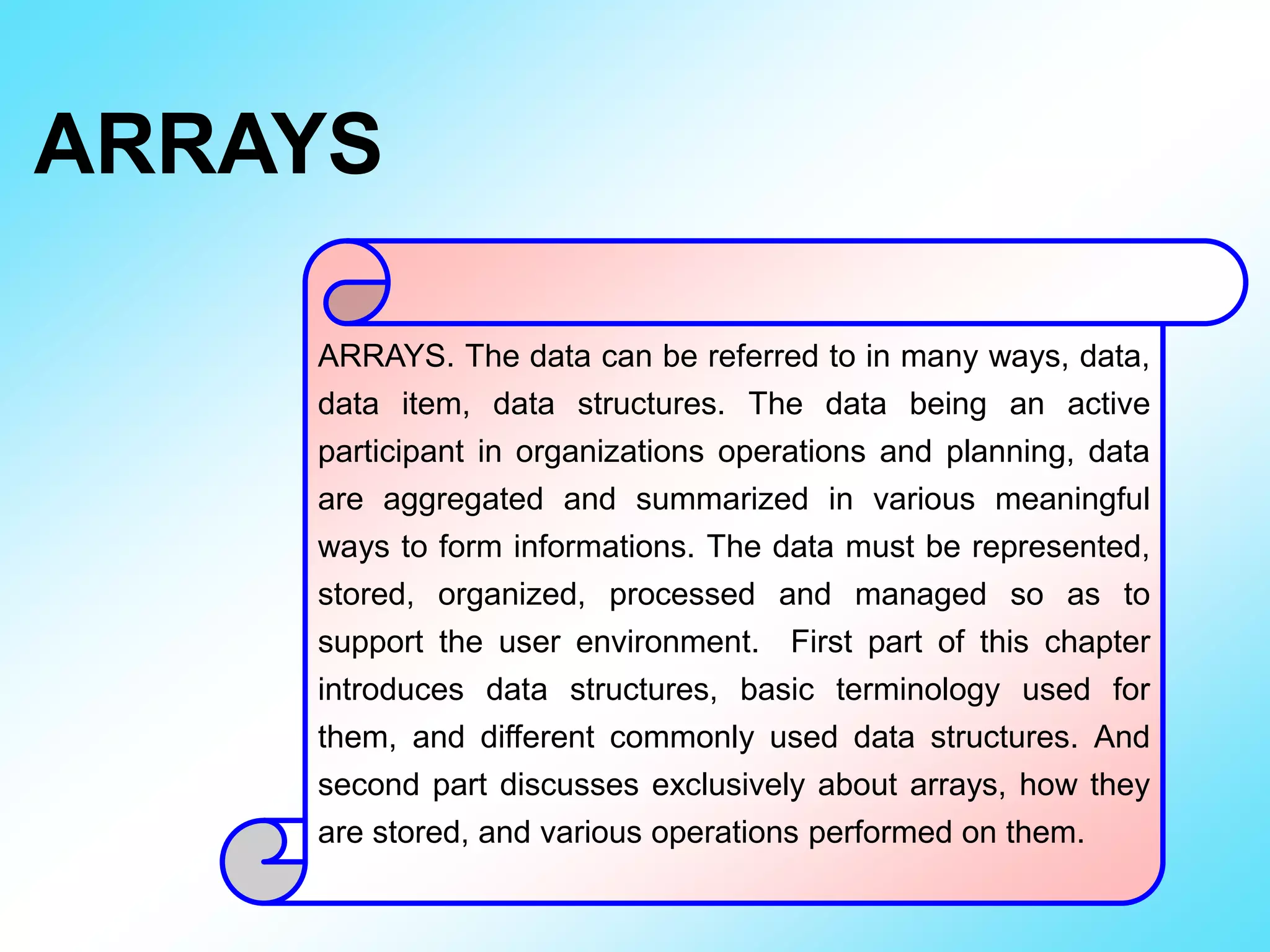
![Arrays. Arrays refers to a named list of finite number of similar elements. Each of the data elements can be referenced by a set of consecutive numbers from 0, 1, 2 to N-1. Arrays can be one dimensional or two dimensional or multi dimensional. int a[10] = { 10 , 20 , 30 , 40 , 50 , 60 , 70 , 80 , 90 , 100 }; int a[3][3] = { { 10, 20, 30 }, { 40, 50, 60 }, { 70, 80, 90 } }; char name[] = “Anil Kumar”; char names[3][20] = { “Anil Kumar”, “Babu Paul”, “Thomas” } char *names [] = { “Anil Kumar”, “Babu”, “Thomas” } student a[3] = { {“Anil”, 100}, {“Babu”, 101}, {“Soman”,102} }; a[0][0] a[0][1] a[0][2] a[1][0] a[1][1] a[1][2] a[2][0] a[2][1] a[2][2] a[0] a[1] a[2] a[3] a[4] a[5] a[6] a[7] a[8] a[9] names[0] name[1] name[2] names[0] name[1] name[2] a[0] a[1] a[2] a[0].name a[0].Roll a[1].name a[1].Roll a[2].name a[2].Roll](https://image.slidesharecdn.com/arrays-200710114741/75/ARRAYS-IN-C-CBSE-AND-STATE-2-COMPUTER-SCIENCE-7-2048.jpg)
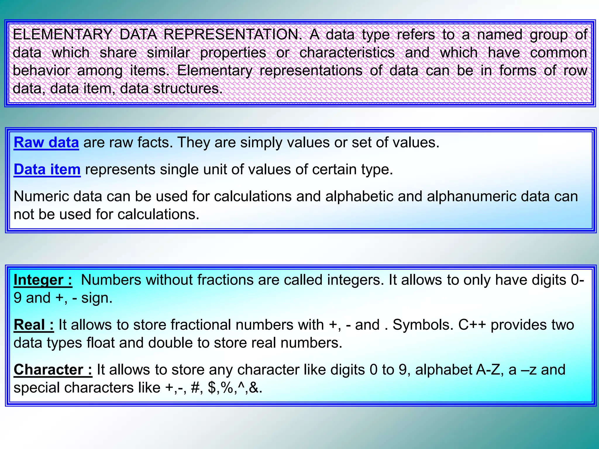
![STRUCTURES. Structures refers to a named collection of data of different types. A structure gathers together different atoms of information that form a given entity. The elements of a structure are referenced by dot operator. When defining a structure, no variables has been created. Objects are created when it declared using TAG name. struct STUDENT { char name[20]; int roll, m1, m2, m3; float per; } a ; Tag Name. Data Members. Declaration of global object ‘a’. class STUDENT { public: char name[20]; int roll, m1, m2, m3; float per; void input(); void output(); } a ; void STUDENT :: input() { } void STUDENT :: output() { } Tag Name. Access Specifier Funtion Definitions main() { STUDENT x, y; strcpy(x.name. “Anil Kumar”); x.Roll = 100; x.m1 = 45; x.m2 = 38; x.m3 = 42; } x name. Elements are referenced by dot operator. // Definition of input () // Definition of output ()](https://image.slidesharecdn.com/arrays-200710114741/75/ARRAYS-IN-C-CBSE-AND-STATE-2-COMPUTER-SCIENCE-8-2048.jpg)
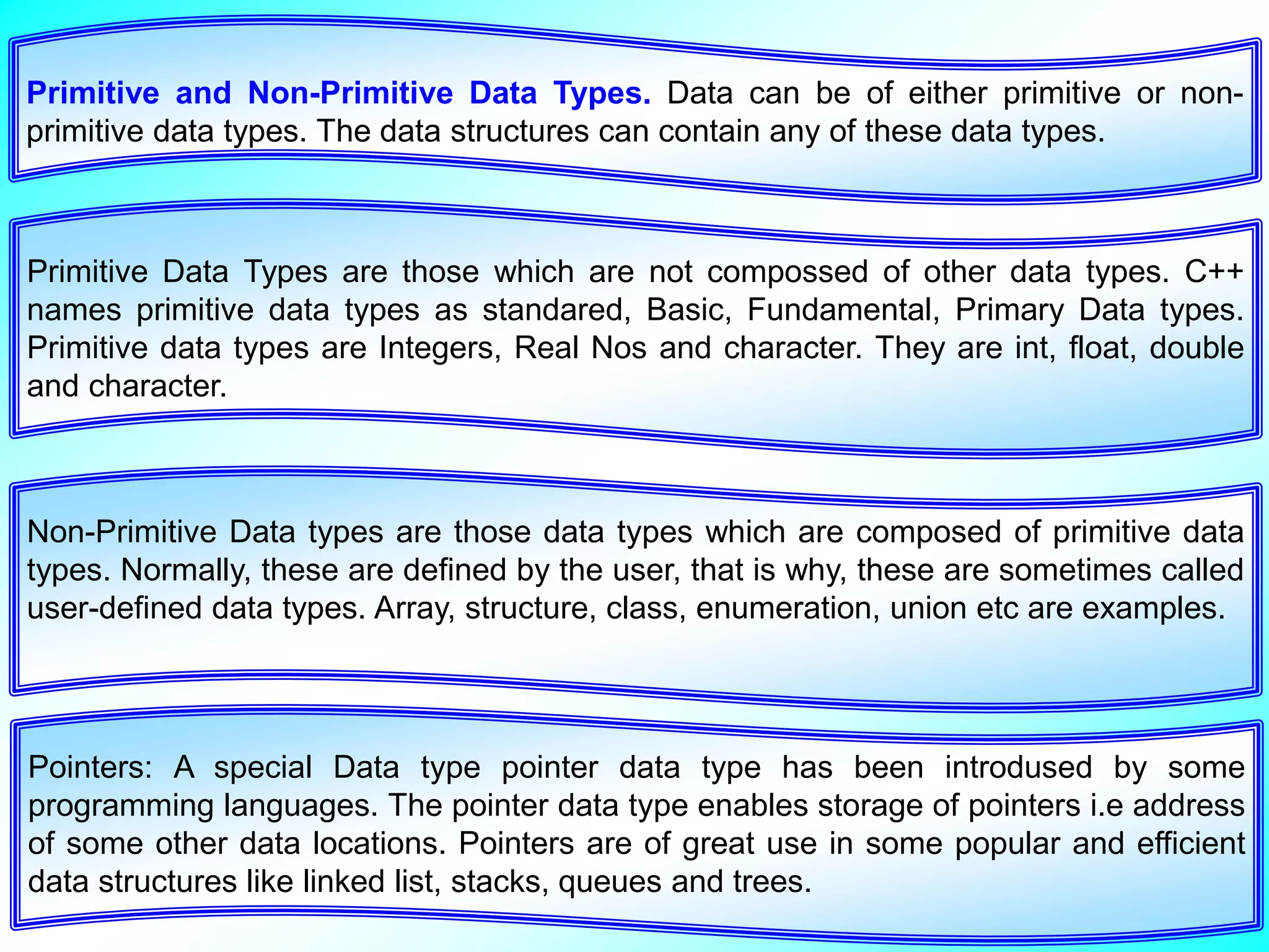
![STACKS. The lists stored and accessed in Last In First Out ( LIFO ) technique is called Stack data structure. In Stacks, insertions and deletions are take place only at one end called the top. Insert an element into the stack is called Push and delete an element from the stack is called Pop. Both Operations are performed at one end of stack named TOP. 3 2 1 Top Show Pushing 6 Show Poping 5 4 Array for storing stack elements. A[0] A[1] A[2] A[3] A[4] A[5] A[6] A[7] Top Show Pushing Show Poping ](https://image.slidesharecdn.com/arrays-200710114741/75/ARRAYS-IN-C-CBSE-AND-STATE-2-COMPUTER-SCIENCE-9-2048.jpg)
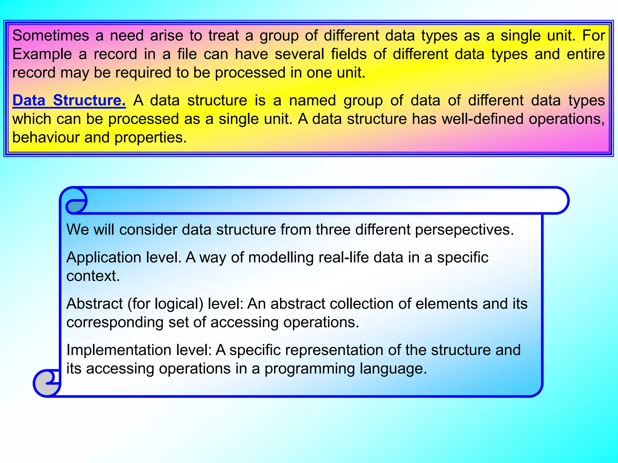
![QUEUE. Queue data structures are FIFO (First In First Out) list, where insertions take place at the ‘rear’ end of the queue and deletion take place at the front end of the queue. Array for storing Queue elements. A[0] A[1] A[2] A[3] A[4] A[5] A[6] A[7] Show Insertion Data will be inserted at the ‘rear’ point of the Queue. Data will be Deleted from the ‘front’ point of the Queue. Q up Show Deletion Rear Front](https://image.slidesharecdn.com/arrays-200710114741/75/ARRAYS-IN-C-CBSE-AND-STATE-2-COMPUTER-SCIENCE-10-2048.jpg)
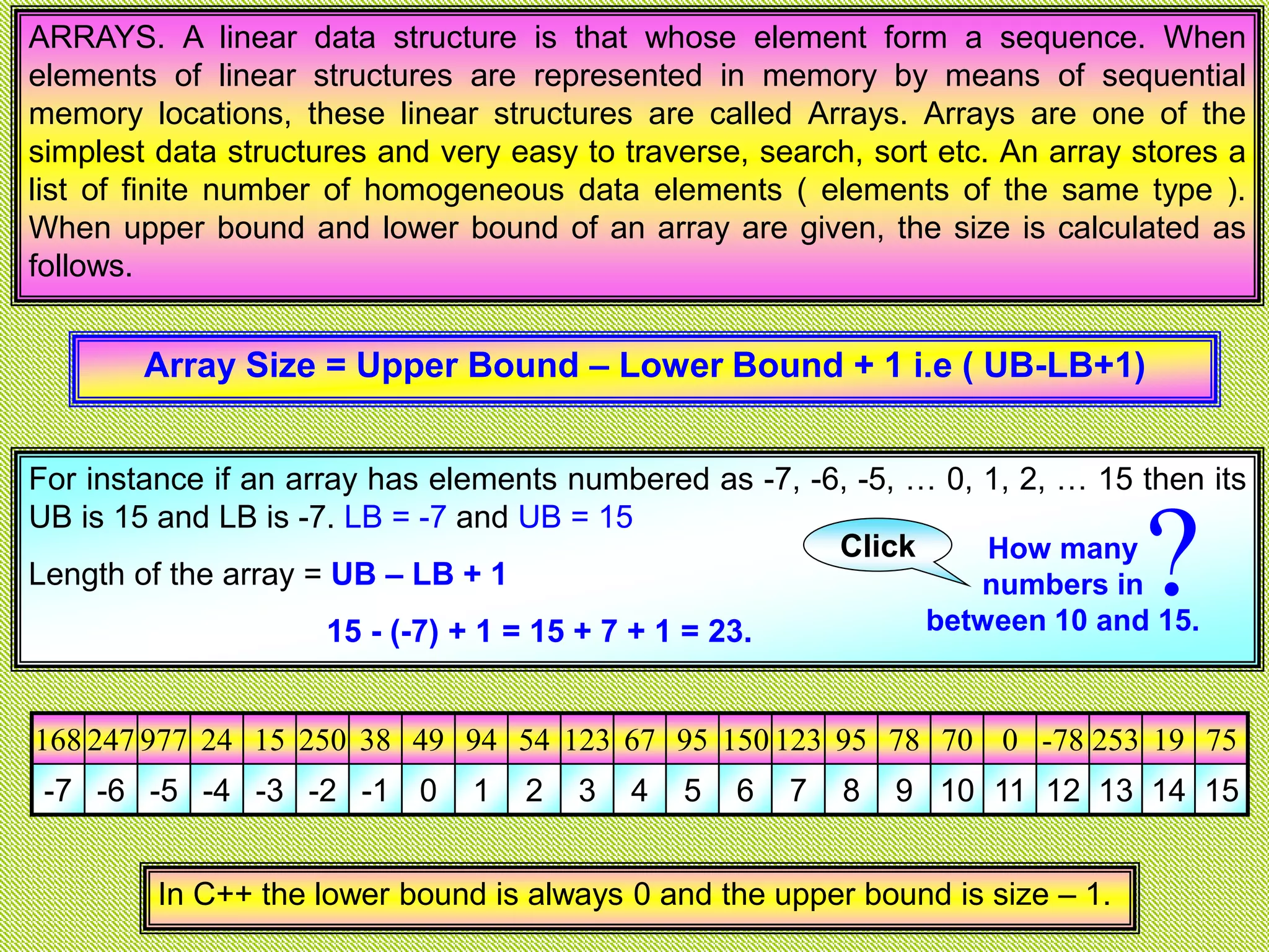
![Let us consider a situation, where we have to accept marks of 50 students of a class, calculate class’s average mark and then calculate the difference of each student’s marks with average marks. We need 50 variables to store marks, one variable to store average marks and another 50 variables to store difference of marks( Class Average - Student’s Mark ). i.e in all 101 variables each having a unique name. But if we use array ( 2 one dimensional Array or 1 two dimensional array ), we only have to remember names of two or three variables. Each element in the array is referenced by giving its position within a [ ] bracket. The number inside the bracket is called subscript or index. The index of an element designates its position in the array. Types of Array. Arrays are of different types. 1. One-dimensional Array considered as a finite homogeneous elements. Eg. A : ARRAY [ -7 .. 15 ] OF INTEGER. (In PASCAL) int a[23]; int a[] = { 168,247,977,24,15,250 }; 2. Multi-Dimensional Array, comprised of elements, each of which is itself an array. B : ARRAY [1..5 : 1..5 ] OF INTEGER int a[10][8]; Array having 10 rows and 8 coloums.](https://image.slidesharecdn.com/arrays-200710114741/75/ARRAYS-IN-C-CBSE-AND-STATE-2-COMPUTER-SCIENCE-15-2048.jpg)
![One dimensional Arrays. Arrays refers to a named list of finite number of similar elements. In memory, array elements are stored in consecutive memory locations. The array itself is given a name and its elements are referred to by their subscript. The notation of an array can be Array Name [ Lower Bound , Upper Bound ] Subscript ranges from L to U. ARRAY A [ -7 .. 15 ] OF INTEGER. Lower bound L = -7 and Upper bound U = 15 In C++, an array being decalred as int a[size]; where the ‘size‘ specifes the number of elements in the array and the subscript ranges from 0 to size-1. 168 247 977 24 15 250 38 49 94 54 123 67 150 123 95 78 70 0 -78 253 19 75 -12 -11 -10 -9 -8 -7 -6 -5 -4 -3 -2 -1 0 1 2 3 4 5 6 7 8 9 Array Length = Upper Bound – Lower Bound + 1 i.e ( UB-LB+1) Index of the element at ‘ith’ position = L + (i – 1) elements forwared. What is the length of following Array ?. L = -12 and U = 9 U – L + 1 = 9 – (-12) + 1 = 9 + 12 + 1 = 22. Lower Bound L Upper Bound UArray Subscript or Index Which value is stored at 5th(i) position and what its subscript ?. Click Me L + (i-1) -12 + (5-1) = 8 15 -8](https://image.slidesharecdn.com/arrays-200710114741/75/ARRAYS-IN-C-CBSE-AND-STATE-2-COMPUTER-SCIENCE-16-2048.jpg)
![Implementation of One-dimensional Arrays in Memory. In memory, one dimensional array are implemented by allocating a sequence of addressed locations so as to accommodate all its elements. The starting address of very first element of the array is called BASE ADDRESS. Array A [ -3 .. 3 ] of integer. If Base Address and size of an element are given, the address of ith element can be calculated as Base Address + Element Size * ( i – L ) Value index Address -3 1000 1001 -2 1002 1003 -1 1004 1005 0 1006 1007 1 1008 1009 2 1010 1011 3 1012 1013 1014 An Array A [ -3 .. 3 ] with subscript range from -3 to 3. What will be the address of A[-1] and A[2], if Base Address is 1000 and size of an elment is 2. L = -3, Base = 1000, Size = 2 Base + Size * ( i – L ) Address of A[-1] : i = -1 = 1000 + 2 * (-1 – (-3)) = 1000 + 2 * (-1 + 3) = 1000 + 2 * 2 = 1004 Address of A[2] : i = 2 = 1000 + 2 * (2 – (-3)) = 1000 + 2 * (2 + 3) = 1000 + 2 * 5 = 1010Show Show 1000+2*(-1-(-3)) 1000 + 2 * 2 1000 + 4 = 1004 1000+2*(2-(-3)) 1000 + 2 * 5 1000 + 10 = 1010 1004 1010](https://image.slidesharecdn.com/arrays-200710114741/75/ARRAYS-IN-C-CBSE-AND-STATE-2-COMPUTER-SCIENCE-17-2048.jpg)
![Value Index Address 1 -12 1000 2 -11 1002 3 -10 1004 4 -9 1006 5 -8 1008 6 -7 1010 7 -6 1012 8 -5 1014 9 -4 1016 10 -3 1018 11 -2 1020 12 -1 1022 13 0 1024 14 1 1026 15 2 1028 16 3 1030 17 4 1032 U Upper bound = 4 L Lower Bound = -12 Base Address = 1000 Legth of the Array = U – L + 1 = 4 – (-12) + 1 = 17 Position of Ith element is calculated as I – Lower Bound + 1. The position of A[-9]. Here I = -9 and L = -12. = -9 – (-12) + 1 = -9 + 12 + 1 = 3 + 1 = 4. A[-3] is the ?th Element in the Array. Click Me A[-6] is the ?th Element in the Array. Click Me A[4] is the ?th Element in the Array. Click Me What will be the address of A[-3] ? . Click Me What will be the address of A[0] ? . Click Me What will be the address of A[-6] ? . Click Me What will be the address of A[3] ?th . Click Me -3 – (-12) + 1 = -3 + 12 + 1 = 9 + 1 = 10. -6 – (-12) + 1 = -6 + 12 + 1 = 6 + 1 = 7. 4 – (-12) + 1 = 4 + 12 + 1 = 16 + 1 = 17.A [ -3 ] : Base address 1000 + 2 * (I - L) = 1000 + 2 * (-3 – (-12)) = `1000+18= 1018A [ 0 ] : Base address 1000 + 2 * (I - L) = 1000 + 2 * (0 – (-12)) = `1000+24= 1024A [ -6 ] : Base address 1000 + 2 * (I - L) = 1000 + 2 * (-6 – (-12)) = `1000+12= 1012A [ 3 ] : Base address 1000 + 2 * (I - L) = 1000 + 2 * (3 – (-12)) = `1000+30= 1030](https://image.slidesharecdn.com/arrays-200710114741/75/ARRAYS-IN-C-CBSE-AND-STATE-2-COMPUTER-SCIENCE-18-2048.jpg)
![Traversal. Traversal in one-dimensional arrays involves processing of all elements (from very first to last element ) one by one. AR[ 1 : U ] if an Array of Integer Consider that all elements have to be printed. 1. ctr = 1 2. Repeat steps 3 and 4 while ctr <= U 3. Print AR[ctr] 4. ctr = ctr + 1 5. end. Basic Operation on One-dimensional Arrays. Algoritham](https://image.slidesharecdn.com/arrays-200710114741/75/ARRAYS-IN-C-CBSE-AND-STATE-2-COMPUTER-SCIENCE-19-2048.jpg)
![# include <iostream.h> # include <conio.h> main() { int a[10] = { 10,20,30,40,50,60,70,80,90,100 }, i, s; cout << “nnThe Given Array is “; for (i=s=0; i<10; i++) { cout << a[i] << “, “; s += a[i]; } cout << “nnnThe Sum of Elements is “ << s; getch(); } Declare an array ‘a’ having 10 integers and initialize elements with 10, 20, 30 .. 100. i Array Index & s sum 100 65525 65524 90 65523 65522 80 65521 65520 70 65519 65518 60 65517 65516 50 65515 65514 40 65513 65512 30 65511 65510 20 65509 65508 10 65507 65506 Let ‘a’ is an array of 10 integers. Print all elements of a and find their sum. a[i] = *(a + i) a[0] = 10 Click Me a[1] = 20 a[2] = 30 a[3] = 40 a[4] = 50 a[5] = 60 a[6] = 70 a[7] = 80 a[8] = 90 a[9] = 100](https://image.slidesharecdn.com/arrays-200710114741/75/ARRAYS-IN-C-CBSE-AND-STATE-2-COMPUTER-SCIENCE-20-2048.jpg)
![Searching. Common two searching algorithms are Linear search and Binary Search. Linear Search. In linear search, each element of the array is compared with the given item to be searched for one by one. This method traverse the array sequentially to locate the given item, is called linear search or sequential search. Algorithm 1. Declare int a[10], i (Array index) and x (item to be search for ?) and flag = 0. 2. Repeat For array index i = 0 to 9 and extract value of a[i] 3. Print the caption “Enter the No to be search for ?” and cin >> x. 4. Repeat for array index i = 0 to 9 If array element a[i] == x then set flag = 1 and break from loop Increment array index. 6. If Flag == 1 then print “Search successful.”, value of array index. Else print “Search Unsuccessfull.”](https://image.slidesharecdn.com/arrays-200710114741/75/ARRAYS-IN-C-CBSE-AND-STATE-2-COMPUTER-SCIENCE-21-2048.jpg)
![Algorithm for Linear Search written Text Book. Step 1. Set ctr = L Step 2. Repeat steps t and 4 while ctr < U Step 3. if Array[ctr] == ITEM then flag = 1 and break. Step 4. else increment value of ctr. Step 5. if flag == 1 then print “The ITEM was found at ‘ctr’ th position.“ Step 6. Elase print “Not Found”.](https://image.slidesharecdn.com/arrays-200710114741/75/ARRAYS-IN-C-CBSE-AND-STATE-2-COMPUTER-SCIENCE-22-2048.jpg)
![# include <iostream.h> main() { int *a, n, i, ITEM, flag = 0; cout << "nnnPlease Enter the Size of the Array "; cin >> n; a = new int[n]; for(i=0; i<n; i++) { cout << "nnPlease Enter " << i << "th No "; cin >> a[i]; } cout << "nnnWhich No You Want To Search for ?. "; cin >> ITEM; for(i=0; i<n; i++) if (a[i] == ITEM) { flag = 1; break; } if(flag == 1) cout << "nnnThe ITEM is present at " << i << " Indes. "; else cout << "nnnItem Was Not Found."; } Value Index/Adr 100 65525 a[9] 65524 90 65523 a[8] 65522 80 65521 a[7] 65520 70 65519 a[6] 65518 60 65517 a[5] 65516 50 65515 a[4] 65514 40 65513 a[3] 65512 30 65511 a[2] 65510 20 65509 a[1] 65508 10 65507 a[0] 65506 Click Me Check whether a[i] == 60 (ITEM) ITEM to be search. a[0] = 10 a[2] = 30 a[3] = 40 a[4] = 50 a[5] = 60 a[1] = 20 flag = 1](https://image.slidesharecdn.com/arrays-200710114741/75/ARRAYS-IN-C-CBSE-AND-STATE-2-COMPUTER-SCIENCE-23-2048.jpg)
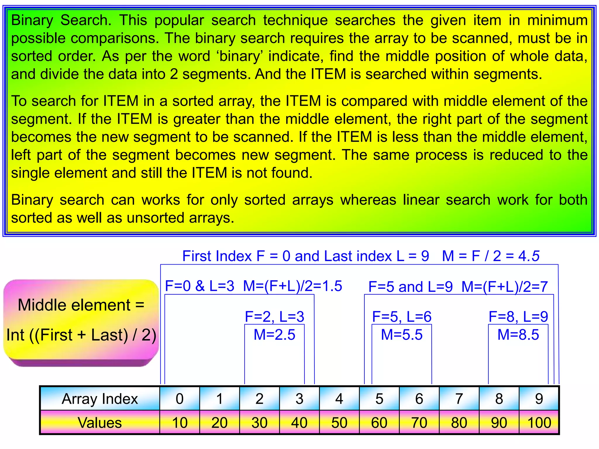
![Algorithm 1. Declare int a[10], searching No ITEM, first F, last L, middle M and FLAG = 0 2. Repeat for Array index L = 0 to 9 and input array elements ( cin >> a[L] ) 3. Ask “Which No You Want to Search For ?” and cin value of ITEM. 4. Let F = 0 and L = 9. 5. Repeat following while First F is <= Last L Calculate middle as M = (F+L) / 2. If middle th element = ITEM then Set Flag = 1 and break from loop. Else if First F is >= Last L then break from loop. Else if ITEM is < A[M] then Last l becomes M – 1. Else First becomes M + 1 6. If FLAG == 1 then Print “The ITEM is Located at Mth Index.” 7. Else Print “The ITEM is Not Found.”](https://image.slidesharecdn.com/arrays-200710114741/75/ARRAYS-IN-C-CBSE-AND-STATE-2-COMPUTER-SCIENCE-25-2048.jpg)
![BINARY SEARCH IN ARRAY. ALGORITHAM Case 1: Array AR[L:U]is stored in ascending order. 1. Set first = L and last = U 2. Repeat Step 3 to 6 while beg < last 3. Mid = int ( (first + last) / 2 ) 4. If ( AR[mid] == ITEM ) then set flag = 1 and break from loop 5. Else if ( ITEM < AR[MID] ) then last = mid – 1 and repeat step from 3 6. Else set first = mid + 1 and repeat step from 3. 7. If flag = 1 then print “Item is present at midth position.” 8. Else print “Not Found.” Case 2: Array AR[L:U]is stored in descending order. 5. Else if ( ITEM < AR[MID] ) then first = mid + 1 and repeat step from 3 6. Else set last = mid - 1 and repeat step from 3.](https://image.slidesharecdn.com/arrays-200710114741/75/ARRAYS-IN-C-CBSE-AND-STATE-2-COMPUTER-SCIENCE-26-2048.jpg)
![# include <iostream.h> main() { int *a, n, F,L,M, ITEM, flag = 0; cout << "nEnter the Size of the Array "; cin >> n; a = new int[n]; cout << "nEnter Nos in Ascending Order. "; for(F=0; F< n; F++) cin >> *(a+F); cout << "nWhich No You Want to Locate for ?. "; cin >> ITEM; F=0; L = n-1; while(1) { M = (F+L)/2; if (a[M] == ITEM) { flag = 1; break; } else if(F>=L) break; else if(ITEM < a[m]) L = M - 1; else F = M + 1; } if(flag) cout << “nGiven No is Present at " << m << " index."; else cout << "nThe Given No is Not Found."; } Value Index/Add 100 a[9] 65524 90 a[8] 65522 80 a[7] 65520 70 a[6] 65518 60 a[5] 65516 50 a[4] 65514 40 a[3] 65512 30 a[2] 65510 20 a[1] 65508 10 a[0] 65506 Click Me F = 0 & L = 9 M = 4 F = 0 & L = 3 M = 1 F = 2 & L = 3 M = 2 F = 3 & L = 3 M = 3 Flag = 1 BINARY SEARCH](https://image.slidesharecdn.com/arrays-200710114741/75/ARRAYS-IN-C-CBSE-AND-STATE-2-COMPUTER-SCIENCE-27-2048.jpg)
![Algoritham First the appropriate position for the ITEM is to be determined. i.e if the appropriate position is I +1 then AR[I] <= ITEM >= AR[I+1]. LST specifies maximum possible index in array, u specifies index of last element in Array. 1. Ctrl = L 2. If LST = U then { print “Overflow” Exit from Program. } 3. If AR[ctr] > ITEM then pos = 1 4. Else Repeat Steps 5 and 6 until ctr >= U 5. If AR[ctr] <= ITEM and ITEM <= ar[ctr+1] then pos = ctr +1 and break; 6. Ctr = ctr + 1 End of repeat 7. If ctr = U then pos = U + 1 8. Ctr = U 9. While ctr >= pos perform step 10 through 11 10. AR[ctr + 1] = AR[ctr] 11. Ctr = ctr – 1 12. AR[pos] = ITEM 13. END Insertion. Insertion of new element in array can be done in two ways. (i) if the array is unordered, the new element is inserted at the end of the array. (ii). If the array is sorted then the new element is inserted at appropriate position. To achieve this, rest of the elements are shifted down. The position of very first element, which is > ITEM is the appropriate position of ITEM.](https://image.slidesharecdn.com/arrays-200710114741/75/ARRAYS-IN-C-CBSE-AND-STATE-2-COMPUTER-SCIENCE-28-2048.jpg)
![Insert 50 Algoritham 1. Declare int a[10], array index i, item to be insert ITEM and Position p 2. Repeat for array index i = 0 to 8 and input a[i] 3. Read the value of ITEM to be insert. 4. Repeat for position P = 0 to n advance by 1. if ( a [P] == ITEM ) break 5. Repeat For i = 9 to i>p, shift a[i-1] to a[i] and decrement i by 1. 6. Assign ITEM at AR[p]. Values 10 20 30 40 Array Index 0 1 2 3 4 5 6 7 8 9 100 Find Position Shift elements 9080706050 Shift all these elements rightwards And Place 50 at a[4] P = 4 Let P = 0 and Advance While a[p] <= ITEM(50) For( I = 9; I>p; I- -) Shift A [ I ] = A [ I-1 ] INSERTION](https://image.slidesharecdn.com/arrays-200710114741/75/ARRAYS-IN-C-CBSE-AND-STATE-2-COMPUTER-SCIENCE-29-2048.jpg)
![# include <iostream.h> # include <conio.h> main() { int *a, n, ITEM, i, p; cout << "nnnEnter the Size of the Array. "; cin >> n; a = new int[n+1]; cout << "nEnter the Elements in Ascending Order. "; for(i=0; i<n; i++) cin >> *(a+i); cout << "nnEnter the New Element "; cin >> ITEM; a[p] = ITEM; cout << "nnThe Array After Insertion "; for(i=0; i<=n; i++) cout << a[i] << ", "; } Value Index/Add a[9] a[8] a[7] a[6] a[5] a[4] 40 a[3] 30 a[2] 20 a[1] 10 a[0] 3000 3000 65524 100 int *a MemoryAllocatedforthearrayA[] for(p=0; a[p] <= ITEM && p<n; p++); Click Me for (i=n; i>p; i--) a[i] = a[i-1]; Click Me 90 80 70 6050 All these Are Lesser than ITEM INSERTION](https://image.slidesharecdn.com/arrays-200710114741/75/ARRAYS-IN-C-CBSE-AND-STATE-2-COMPUTER-SCIENCE-30-2048.jpg)
![DELETION. The element to be deleted is first searched for in the array using one of the search techniques, i.e. either linear or binary search. If the search is successful , the element is removed and rest of the element are shifted so as to keep the order of the array undisturbed. If the elements are shifted downwards or rightwards, then the unused (free space) elements are available in the beginning of the array otherwise free space is available at the end of the array. Case 1. Shifting upwards or in left side. 1. Ctr = pos 2. Repeat steps 3 and 4 until ctr >= U 3. AR[ctr] = AR[ctr+1] 4. Ctr = ctr + 1 Case 2. Shifting downwards or in right side. 1. Ctr = pos 2. Repeat steps 3 and 4 until ctr <= 1 3. AR[ctr] = AR[ctr-1] 4. Ctr = ctr - 1 Consider that ITEM’s search in array AR is successful at location pos.](https://image.slidesharecdn.com/arrays-200710114741/75/ARRAYS-IN-C-CBSE-AND-STATE-2-COMPUTER-SCIENCE-31-2048.jpg)
![ALGORITHM OF DELETION. 1. Declare int a[10], array index ‘i’, ITEM to be Delete and its position P. 2. Input each element a [ i ] for array index i = 0 to 9 3. Input the value of ITEM, which will be Delete from the array. 4. Repeat bellow statement for array Index p = 0 to 9, if a [ p ] == ITEM then break. Now ‘p’ is the position of the element we want to remove. 5. Repeat for i = p to 9 increment by 1, Shift a [ i + 1 ] to a [ i ]. To get space at Right end of the Array. OR 5. Repeat for I = p to 1 decrement by 1 Shift a [ i – 1 ] to a [ i ]. To get space at Left end of the array. 6. Repeat for array index i = 0 to 8 Print array element a [ i ]. 7. Stop.](https://image.slidesharecdn.com/arrays-200710114741/75/ARRAYS-IN-C-CBSE-AND-STATE-2-COMPUTER-SCIENCE-32-2048.jpg)
![Delete 45 Values 10 20 30 40 Array Index 0 1 2 3 4 5 6 7 8 9 Find Position Shift elements 45 50 To get Space at Left end of the Array. Shift elements left of ‘p’ rightwards. For(I = p; i>1; i--) A [ I ] = A [ I - 1 ] A [ 0 ] = 0 To Delete an element from an array, Shift either left or right elements into its position. 60 70 80 90 To get Space at Right end of the Array. Shift elements rightt of ‘p’ leftwards. For(I = p; I <= 8; i++) A [ I ] = A [ I + 1 ] A [ 9 ] = 0 For (P=0; P<10; P++) If a[p] = 50 then break; For( I = p; I <= 8; I++) Shift A [ I ] = A [ I + 1 ] ](https://image.slidesharecdn.com/arrays-200710114741/75/ARRAYS-IN-C-CBSE-AND-STATE-2-COMPUTER-SCIENCE-33-2048.jpg)
![# include <iostream.h> main() { int *a, n, ITEM, i, p; cout << "nEnter the Size of the Array. "; cin >> n; a = new int[n]; cout << "nEnter the Elements in Ascending Order. "; for(i=0; i<n; i++) cin >> *(a+i); cout << "nEnter the No to be Delete ? "; cin >> ITEM; if (p==n) cout << "n ITEM Not Found."; else { a[n-1] = 0; cout << "nThe Array After Deletion "; for(i=0; i<n; i++) cout << a[i] << ", "; } } Value Index/Add 90 a[9] 80 a[8] 70 a[7] 60 a[6] 50 a[5] 45 a[4] 40 a[3] 30 a[2] 20 a[1] 10 a[0] 3000 3000 65524MemoryAllocatedforthearrayA[] for (i=p; i<n; i++) a[i] = a[i+1]; Click Me for(p=0; p < n; p++) if (a[p] == ITEM) break; Click Me 50 60 70 80 90 A [ I ] != 45 DELETION.](https://image.slidesharecdn.com/arrays-200710114741/75/ARRAYS-IN-C-CBSE-AND-STATE-2-COMPUTER-SCIENCE-34-2048.jpg)
![Consider a 1–D array ‘A’ containing 100 integers. Develop an algorithm for following. 1. Remove all occurrence of a given integer. 2. Shift the elements of the array to the right so that used space is available at the left. 3. Fill the unused space by 0. Solution. As nothing is mentioned whether array is sorted or not, use linear search. 1. Read ITEM 2. Ctr = 0. 3. Repeat steps 4 through 11 until ctr > U 4. If AR[ctr] = ITEM then 5. { pos = ctr 6. ctr2 = pos 7. Repeat steps 8 through 9 until ctr2 <= 0 8. AR[ctr2] = AR[ctr2-1] 9. ctr2 = ctr2 – 1 /* End of Repeat (Step 7) */ 10. a[1] = 0 } /* End of Repeat (Step 4) 11. Ctr = ctr +1 12. If ctr > U then print “Sorry ! Element not found. !!”](https://image.slidesharecdn.com/arrays-200710114741/75/ARRAYS-IN-C-CBSE-AND-STATE-2-COMPUTER-SCIENCE-35-2048.jpg)
![SORTING. Sorting of an array means arranging the array elements in a specified order. i.e either ascending or descending order. The three very common techniques are selection Sort, Bubble Sort and insertion sort. Selection Sort. In this technique, find the next smallest element in the remaining part of the array and brings it at its appropriate position. That is, Take an element (key) , and find the smallest element in the remaining part of the array, and exchange key and smallest element. Algorithm. 1. Repeat Steps 2 to 5 For I = L to U, increment I by 1. 2. Small = AR[I] and Po`s = I 3. Repeat 4th step For J = I + 1 to U, increment J by 1. 4. If AR[J] < AR[I] then small = AR[J] and POS = J 5. If I != POS then temp = AR[I], AR[I] = small, AR[POS] = temp](https://image.slidesharecdn.com/arrays-200710114741/75/ARRAYS-IN-C-CBSE-AND-STATE-2-COMPUTER-SCIENCE-36-2048.jpg)
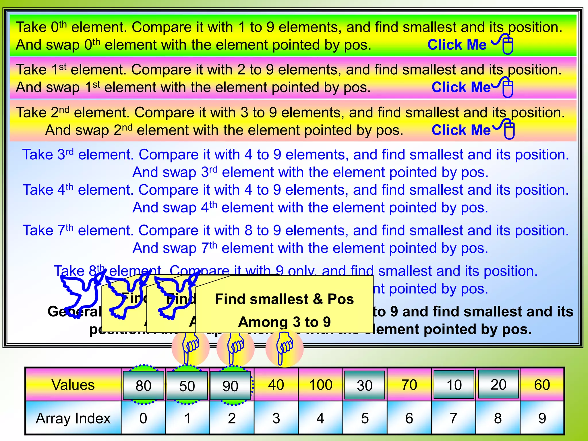
![1. Declare int a[10], array index I, j, smallest No: s and its position Pos. 2. Repeat for array index I = 0 to 9 and input value of a[i]. A) Let small = a [ I ], and pos = I; B) Repeat for j = I + 1 to 9 and If ( a[ j ] < small ) then small = a[ j ] and Pos = j C) If small < a[i] then j (temp) = a[i], a[i] = small, a[pos] = j(temp) 4. Repeat for array index I = 0 to 9 and print a[i]. Values 80 50 90 40 100 30 70 10 20 60 Array Index 0 1 2 3 4 5 6 7 8 9 3. Repeat following for array index I = 0 to 8. Click Me 80 For( j=i+1; j<10; j++ ) if( small < a[j] ) { small = a[j], pos = j; } 50 For( j=i+1; j<10; j++ ) if( small < a[j] ) { small = a[j], pos = j; } 90 40 100 30 70 10 20 For( j=i+1; j<10; j++ ) if( small < a[j] ) { small = a[j], pos = j; } For( j=i+1; j<10; j++ ) if( small < a[j] ) { small = a[j], pos = j; } For( j=i+1; j<10; j++ ) if( small < a[j] ) { small = a[j], pos = j; } For( j=i+1; j<10; j++ ) if( small < a[j] ) { small = a[j], pos = j; } SELECTION SORT.](https://image.slidesharecdn.com/arrays-200710114741/75/ARRAYS-IN-C-CBSE-AND-STATE-2-COMPUTER-SCIENCE-38-2048.jpg)
![# include <iostream.h> # include <conio.h> void selsort(int *x, int n) { int i, j, small, pos, temp; for(i=0; i<n-1; i++) { small = x[i]; pos = i; for(j=i+1; j<n; j++) { if(x[j] < small) { small = x[j]; pos = j; } } if(pos != i) { temp = x[i]; x[i] = x[pos]; x[pos] = temp; } } } main() { int *a, n, i; cout << "nEnter the Size of the Array "; cin >> n; a = new int[n]; cout << "nnnEnter the elements "; for(i=0; i<n; i++) cin >> a[i]; selsort(a, n); cout << "nnnThe Sorted Array is "; for(i=0; i<n; i++) cout << a[i] << ", "; getch(); } Take ith element, Compare it with i+1 to 9 and find smallest and its position. And swap ith element with the element pointed by pos. For j= i+1 to n Finding smallest No ](https://image.slidesharecdn.com/arrays-200710114741/75/ARRAYS-IN-C-CBSE-AND-STATE-2-COMPUTER-SCIENCE-39-2048.jpg)
![Bubble Sort. The basic idea of bubble sort is to compare two adjoining values and exchange them if they are not in proper order. ALGORITHM 1. For I = L to U { 2. for J = L to (U-1)-1 { 3. if AR[J] > AR[J+1] THEN { 4. TEMP = AR [ J ] 5. AR [ J ] = AR [ J + 1 ] 6. AR [ J + 1 ] = TEMP } } } 7. END.](https://image.slidesharecdn.com/arrays-200710114741/75/ARRAYS-IN-C-CBSE-AND-STATE-2-COMPUTER-SCIENCE-40-2048.jpg)
![ALGORITHM OF BUBBLE SORT Take an element, Compare it with adjoining elements and swap elements if needed. After each PASS, the heaviest elements comes to end. Total N – 1 Pass will needed to Sort an entire Array. PASS 1 : If 0th element is < than 1st element then Swap. If 1st element is < than 2nd element then Swap. If 2nd element is < than 3rd element then Swap. If 3rd element is < than 4th element then Swap. If 4th element is < than 5th element then Swap. If 5th element is < than 6th element then Swap. If 6th element is < than 7th element then Swap. If 7th element is < than 8th element then Swap. If 8th element is < than 9th element then Swap. After first PASS the heaviest element comes at End. Click Me PASS 2 : If 0th element is < than 1st element then Swap. If 1st element is < than 2nd element then Swap. If 2nd element is < than 3rd element then Swap. If 3rd element is < than 4th element then Swap. If 4th element is < than 5th element then Swap. If 5th element is < than 6th element then Swap. If 6th element is < than 7th element then Swap. If 7th element is < than 8th element then Swap. After second PASS the second heaviest element comes at appropriate position. Click Me Values 80 50 90 40 100 30 70 10 20 60 Array Index 0 1 2 3 4 5 6 7 8 9 FOR(J=0; J<N-pass; J++) IF A[J+1] < A[J} THEN SWAP( A[J], A[J+1] ) 100 FOR(J=0; J<N-pass; J++) IF A[J+1] < A[J} THEN SWAP( A[J], A[J+1] ) 90](https://image.slidesharecdn.com/arrays-200710114741/75/ARRAYS-IN-C-CBSE-AND-STATE-2-COMPUTER-SCIENCE-41-2048.jpg)
![# include <iostream.h> # include <conio.h> void bubble(int *x, int n) { int i, j,temp; for(i=0; i<n-1; i++) { for(j=0; j<n-i; j++) { if(x[j] > x[j+1]) { temp = x[j]; x[j] = x[j+1]; x[j+1] = temp; } } } } main() { int *a, n, i; cout << "nEnter the Size of the Array "; cin >> n; a = new int[n]; cout << "nnnEnter the elements "; for(i=0; i<n; i++) cin >> a[i]; bubble(a, n); cout << "nnnThe Sorted Array is "; for(i=0; i<n; i++) cout << a[i] << ", "; getch(); } BUBBLE SORT](https://image.slidesharecdn.com/arrays-200710114741/75/ARRAYS-IN-C-CBSE-AND-STATE-2-COMPUTER-SCIENCE-42-2048.jpg)
![Insertion Sort. In insertion Sort, each successive elements are picked and insert at appropriate position in the previously sorted left part of the array. In this technique, scan whole array AR from AR[0] to AR[U-1], insert each element AR[I] into its proper position in the previously sorted subarray AR[0], AR[1], AR[2] .. AR[N-1]. To make AR[0] the sentinel element by storing minimum possible integer value. 1. AR[0] = ,minimum integer value. 2. Repeat Steps 3 through 8 for K = 1, 2, 3, … N-1 3. Temp = AR[K] 4. Ptr = K – 1 5. Repeat Steps from 6 and 7 while temp < AR[ptr] 6. AR[ptr+1] = AR[ptr] 7. Ptr = ptr – 1 8. AR[ptr+1] = temp 9. End.](https://image.slidesharecdn.com/arrays-200710114741/75/ARRAYS-IN-C-CBSE-AND-STATE-2-COMPUTER-SCIENCE-43-2048.jpg)
![Algorithm 1. Declare int A [ 10 ], array Index I, Position P, key; 2. Repeat for array index I = 0 to 9 and input value of a[i]. 3. Repeat following for I = 1 to 9 A) Assign Key = A [ I ] and P = I - 1 B) Repeat while A [ P ] > Key and P >= 0 A [ P+1 ] = A[P], Decrement P by 1. C) A [P+1] = key 4. Repeat for array index I = 0 to 9 Print A [ I ] Values 10 30 40 50 60 20 70 80 90 100 Array Index 0 1 2 3 4 5 6 7 8 9 Show 5th Pass 60 P = 4 Key = A) Assign Key = A [ I ] and P = I - 1 20 Shift these elements to Right While(A[P]>Key && P >=0) { A[P+1] = A[P]; P--; } 504030 20 ALGORITHM OF INSERTION SORT](https://image.slidesharecdn.com/arrays-200710114741/75/ARRAYS-IN-C-CBSE-AND-STATE-2-COMPUTER-SCIENCE-44-2048.jpg)
![# include <iostream.h> # include <conio.h> void ins_sort(int *x, int n) { int i, j,temp, key; for(i=1; i<n; i++) { key = x[i]; j = i-1; while(x[j] > key && j>=0) { x[j+1] = x[j]; j--; } if(j+1 != i) { x[j+1] = key; } } } main() { int *a, n, i; cout << "nEnter the Size of the Array "; cin >> n; n = 10; a = new int[n]; cout << "nnnEnter the elements "; for(i=0; i<n; i++) cin >> a[i]; ins_sort(a, n); cout << "nnnThe Sorted Array is "; for(i=0; i<n; i++) cout << a[i] << ", "; getch(); } INSERTION SORT](https://image.slidesharecdn.com/arrays-200710114741/75/ARRAYS-IN-C-CBSE-AND-STATE-2-COMPUTER-SCIENCE-45-2048.jpg)
![Merging. Merging means combine elements of two arrays to form a new array. Simplest way of merging two array is that first copy all the elements of one array into new array and then copy all the elements of other array into new array. If you want the resultant array to be sorted, you can sort the resultant array. Another popular technique to get a sorted resultant array is sorting while merging. It is MREGE SORT. If Both array having elements, Compare each elements of both arrays and assign smallest element in the third array. At last some elements will remains in any array. Remaining elements of that array are copied into the third array. Aarray index A[0] A[1] A[2] A[3] Value 5 15 25 35 Aarray index A[0] A[1] A[2] A[3] A[4] A[5] A[6] A[7] A[8] A[9] Value 5 10 15 20 25 30 35 40 50 60 Aarray index A[0] A[1] A[2] A[3] A[4] A[5] Value 10 20 30 40 50 60 5 15 25 35 10 20 30 40 50 Show 60](https://image.slidesharecdn.com/arrays-200710114741/75/ARRAYS-IN-C-CBSE-AND-STATE-2-COMPUTER-SCIENCE-46-2048.jpg)
![Both Arrays A and B are in ascending order, C has to be in ascending order. 1. Ctr_A = L1, ctr_B = L2, ctr_C = L3 2. While Ctr_A <= U1 and ctr_B <= U2 performs steps 3 to 5. 3. If A[ctr_A] < B[ctr_B] then C[ctr_c] = A[ctr_A] Ctr_A = ctr_A + 1 4. Else C[ctr_C] = B[Ctr_B] Ctr_B = ctr_B + 1 5. Ctr_C = Ctr_C + 1 6. While Ctr_A < U1 C[ctr_c] = A[ctr_A] Ctr_A = ctr_A + 1 Ctr_C = Ctr_C + 1 7. While Ctr_B < U2 C[ctr_C] = B[Ctr_B] Ctr_B = ctr_B + 1 Ctr_C = Ctr_C + 1 ALGORITHM OF MERGE SORT](https://image.slidesharecdn.com/arrays-200710114741/75/ARRAYS-IN-C-CBSE-AND-STATE-2-COMPUTER-SCIENCE-47-2048.jpg)
![Both Arrays A and B are in ascending order, C has to be in ascending order. 1. Declare A[5], B[6], C[11], AI (index of A), BI (index of B), CI (index of C) 2. Repeat for AI = 0 to 4 incremented by 1 and input A[AI]. 3. Repeat for BI = 0 to 5 incremented by 1 and input B[BI]. 4. Repeat following While both array having elements ie While( AI <= 4 and BI <= 5) (While Index of Array A is less than its size and Index of Array B is less than its size) If ( A[AI] < B[BI] ) then C[CI] = A[AI] and increment AI by 1 Else C[CI] = B[BI] and increment BI by 1 Increment CI by 1. 6. While Array A having elements ie. While ( AI <= its size 4) C[CI] = A[AI], increment AI and CI by 1 6. While Array A having elements ie. While ( BI <= its size 5) C[CI] = B[BI], increment BI and CI by 1 7. Repeat for CI = 0 to 10 incremented by 1 and print C[CI] ALGORITHM OF MERGE SORT](https://image.slidesharecdn.com/arrays-200710114741/75/ARRAYS-IN-C-CBSE-AND-STATE-2-COMPUTER-SCIENCE-48-2048.jpg)
![# include <iostream.h> # include <conio.h> void merge (int *a, int *b, int *c, int m, int n) { int ai=0, bi=0, ci=0; while( ai<m && bi < n) { if(a[ai] < b[bi]) { c[ci] = a[ai]; ai++; } else { c[ci] = b[bi]; bi++; } ci++; } while(ai<m) { c[ci] = a[ai]; ai++; ci++; } while(bi<n) { c[ci] = b[bi]; bi++; ci++; } } MERGE SORT main() { int *a, *b, *c, m, n, i; cout << "nEnter the Size of the Array A "; cin >> m; cout << "nEnter the Size of the Array B "; cin >> n; a = new int[m]; b = new int[n]; c = new int[m+n]; cout<<“nEnter 1st Array in ascending Order"; for(i=0; i<m; i++) cin >> a[i]; cout<<“nEnter 2nd Array in ascending Order"; for(i=0; i<n; i++) cin >> b[i]; merge (a,b,c,m,n); cout << "nnnThe Sorted Array is "; for(i=0; i<m+n; i++) cout << c[i] << ", "; getch(); }](https://image.slidesharecdn.com/arrays-200710114741/75/ARRAYS-IN-C-CBSE-AND-STATE-2-COMPUTER-SCIENCE-49-2048.jpg)
![Example 9.8. Suppose A, B, C are arrays of integers of size m, n, m + n respectively. The numbers in arrays A appear in ascending order and B is in descending order. Given an algorithm to produce a third array C, containing all the data of array A and B in descending order. 1. Let Ctr_A = 0, Ctr_B = N-1, Ctr_C = 0 2. While Ctr_A < M and Ctr_B >= 0 performs Step 3 to 5 3. If A[Ctr_A] < B[Ctr_B] then C[Ctr_C] = A[Ctr_A], Ctr_A = Ctr_A + 1 4. Else C[Ctr_C] = B[Ctr_B], Ctr_B = Ctr_B - 1 5. Ctr_C = Ctr_C + 1 6. While Ctr_A < M then C[Ctr_C] = A[Ctr_A] Ctr_A = Ctr_A + 1 Ctr_C = Ctr_C + 1 7. While Ctr_B >=0 then C[Ctr_C] = B[Ctr_B] Ctr_B = Ctr_B – 1 Ctr_C = Ctr_C + 1](https://image.slidesharecdn.com/arrays-200710114741/75/ARRAYS-IN-C-CBSE-AND-STATE-2-COMPUTER-SCIENCE-50-2048.jpg)
![Example 9.9 Suppose A, B, C are arrays of integers of size m, n, m + n respectively. Array A is stored in ascending order and B is in Descending Order. Give an algorithm to produce a third array C containing all the data of A and B in descending Order. 1. Let Ctr_A = 0, Ctr_B = N - 1, Ctr_C = (M + N) - 1 2. While Ctr_A < M and Ctr_B >= 0 performs Step 3 to 5 3. If A[Ctr_A] < B[Ctr_B] then C[Ctr_C] = A[Ctr_A] Ctr_A = Ctr_A + 1 4. Else C[Ctr_C] = B[Ctr_B] Ctr_B = Ctr_B - 1 5. Ctr_C = Ctr_C - 1 6. While Ctr_A < M then C[Ctr_C] = A[Ctr_A] Ctr_A = Ctr_A + 1 Ctr_C = Ctr_C – 1 7. While Ctr_B >=0 then C[Ctr_C] = B[Ctr_B] Ctr_B = Ctr_B – 1 Ctr_C = Ctr_C – 1](https://image.slidesharecdn.com/arrays-200710114741/75/ARRAYS-IN-C-CBSE-AND-STATE-2-COMPUTER-SCIENCE-51-2048.jpg)
![TWO DIMENSIONAL ARRAYS. A two dimensional array is an array in which each row is itself an array. An array A[1..M, 1..N] is an array having M rows and N columns. And containing M x N elements. The No of elements in a 2-D array can be determined by (i) Calculating number of rows and number of columns and then (ii) by multiplying number of rows with no of columns. Consider an Array A[-3..5, -2..7] U Upper bound and L Lower Bound. No of Rows = UROW – LROW + 1 = 5 – (-3) + 1 = 9 No of Columns = UCOLUMN – LCOLUMN + 1 = 7 – (-2) + 1 = 10 Implementation of two-dimensional Array in Memory. While storing the elements of a 2-D array in memory, these are allocated contiguous locations. There for the array is linearized so as to enable their storage. There are 2 alternative for linearzation of a 2-D array. Row Major and Column Major. 1. Row Major 2. Column Major](https://image.slidesharecdn.com/arrays-200710114741/75/ARRAYS-IN-C-CBSE-AND-STATE-2-COMPUTER-SCIENCE-52-2048.jpg)
![4021 4020 4019 4018 4017 4016 4015 4014 4013 4011 4010 4009 4008 4007 4005 4004 4003 4002 4001 No of Rows = UROW – LROW + 1 = 2 – 0 + 1 = 3 No of Columns = UCOL – LCOL + 1 = 2 – 0 + 1 = 3 Row 2 Row 0 Row 1 Row 2 2 1 3 4000 4 6 5 4006 8 7 9 4012 10 2 1 2 3 4 5 6 7 8 9 1 2 3 4 5 6 7 8 9 Row Major Implementation. This linearzation technique stores firstly the first row of the array, then the second row of the array, then the third row of the array Columns Address of A[ I, J ] = Base + W ( N (I-1) + (J-1) ) Where (I-1) No of rows before Ith Row. (J-1) No of Columns before Jth Column. N * ( I - 1 ) Total No of elements in previous Rows. N * ( I - 1 ) + J Total No of elements to be advance. W * (N * ( I - 1 ) + J) Total No of Bytes to be advance. Address of A[I,J] = BASE + W * ( N * ( I-1 ) + J ) i.e Advance W * ( N * ( I-1 ) + J ) bytes from BASE. Row 0 Row 1 ROW MAJOR](https://image.slidesharecdn.com/arrays-200710114741/75/ARRAYS-IN-C-CBSE-AND-STATE-2-COMPUTER-SCIENCE-53-2048.jpg)
![General form for address calculation of A [ I, J ] element of Array A [ LR : UR, LC : UC ] with base Address B and element size W bytes is Col -1 Col 0 Col 1 Col 2 Col 3 Row 4 100 102 104 106 108 Row 5 110 112 114 116 118 Row 6 120 122 124 126 128 Row 7 130 132 134 136 138 Example 9.11. A 2-D array A[4 : 7, -1 : 3] requires 2 Bytes of storage space for each element. Calculate the address of A[6,2] if BASE address is 100. Base = 100 Size W = 2 bytes LROW = 4 LCOL = -1 UCOL = 3 I = 6 J = 2 No of Columns ( N ) = UCOL – LCOL + 1 = 3 – (-1) + 1 = 3 + 1 + 1 = 5 A [ I, J ] = B + W ( N ( I – LROW ) + ( J – LCOL ) ) = 100 + 2 ( 5 * ( 6 – 4 ) + ( 2 – ( -1 )) ) = 100 + 2 ( 5 * 2 + 3 ) = 100 + 2 * 13 = 126 ADDRESS OF A [ 6 : 2 ] A[ I, J ] = Base + W ( N ( I – LROW ) + ( J – LCOL) ) ROW MAJOR](https://image.slidesharecdn.com/arrays-200710114741/75/ARRAYS-IN-C-CBSE-AND-STATE-2-COMPUTER-SCIENCE-54-2048.jpg)
![Col 1 Col 2 Col 3 Col 4 Col 5 Row 1 150 152 154 156 158 Row 2 160 162 164 166 168 Row 3 170 172 174 176 178 Row 4 180 182 184 186 188 Example 9.12. X is 2-D array [10 X 5]. Each element of the array is stored in 2 memory locations. If X[1,1] begins at addrerss 150. Find the location of X[3,4]. Base = 150 Size W = 2 bytes LROW = LCOL = -1 UCOL = 5 I = 3 J = 4 No of Columns ( N ) = UCOL – LCOL + 1 = 5 – 1 + 1 = 5 A [ I, J ] = B + W ( N ( I – LROW ) + ( J – LCOL ) ) = 150 + 2 ( 5 * ( 3 – 1 ) + ( 4 – 1 ) ) = 150 + 2 ( 5 * 2 + 3 ) = 150 + 2 * 13 = 176 ADDRESS OF X [ 3 : 4 ] A[ I, J ] = Base + W ( N ( I – LROW ) + ( J – LCOL) ) ROW MAJOR](https://image.slidesharecdn.com/arrays-200710114741/75/ARRAYS-IN-C-CBSE-AND-STATE-2-COMPUTER-SCIENCE-55-2048.jpg)
![4021 4020 4019 4018 4017 4016 4015 4014 4013 4011 4010 4009 4008 4007 4005 4004 4003 4002 4001 General form for address calculation of A [ I, J ] element of Array A [ LR : UR, LC : UC ] with base Address B and element size W bytes is B + W ( M ( J – LCOL ) + ( I – LROW) ) Col 2 Row 0 Row 1 Row 2 4 1 7 4000 2 8 5 4006 6 3 9 4012 1 2 3 4 5 6 7 8 9 2 5 8 3 6 9 Column Major. This linearzation technique stores firstly the first column, then the second column then the third column and so forth. Columns Where M No of elements in each columns. ( No of Rows ) M ( J – LCOL ) No of elements before Jth Column. ( I – LROW ) No of elements before Ith Row. M ( J – LCOL ) + ( I – LROW ) Total No of elements before A [ I, J ] W ( M ( J – LCOL ) + ( I – LROW ) ) To tal No of Bytes. A [ I , J ] = BASE + W * ( M * ( J – LCOL ) + ( I - LROW ) i.e Advance W * ( M * ( J – LCOL ) + ( I - LROW ) bytes from BASE. Col 0 Col 1 1 4 7 2 1 0 B + W ( M ( J – LCOL ) + ( I – LROW ) )](https://image.slidesharecdn.com/arrays-200710114741/75/ARRAYS-IN-C-CBSE-AND-STATE-2-COMPUTER-SCIENCE-56-2048.jpg)
![Col 10 Col 11 Col 12 Col 13 Col 14 ….. Col 30 ….. Col 35 Row -20 500 541 582 623 664 1320 1525 Row -19 501 542 583 624 665 1321 1526 …….. Row 0 1340 …….. Row 20 540 581 622 663 704 1360 1565 Example 9.13. Each element of the array A [ -20 : 20, 10 : 35 ] requires 1 byte of storage.If the array is stored in column major order beginning location 500. Determine the location of A [ 0, 30 ]. Base = 500, Size W = 1 byte, LROW = -20, LCOL = 10, UROW = 20, I = 0, J = 30 No of Rows ( M ) = UROW – LROW + 1 = 20 – ( -20 ) + 1 = 41 A [ I, J ] = B + W ( M ( J – LCOL ) + ( I – LROW ) ) = 500 + 1 ( 41 * ( 30 – 10 ) + ( 0 – ( -20 )) ) = 500 + 1 ( 41 * 20 + 20 ) = 500 + 820 + 20 = 1340 A[ I, J ] = Base + W ( M ( J – LCOL ) + ( I – LROW) ) Column 10, 11, .. 29 = 20 Columns Row -20, -19, -18 … 0 = 20 Rows 1 Column has 41 elements 20 column has 41 * 20 = 820 + 20 elements forward = 840 = 500 + 840 = 1340.](https://image.slidesharecdn.com/arrays-200710114741/75/ARRAYS-IN-C-CBSE-AND-STATE-2-COMPUTER-SCIENCE-57-2048.jpg)
![Example 9.14. Each element of an array A [ -15 : 20, 20 : 45 ] require one byte of storage. Determine the location of A [ 0, 40 ] if its base address = 1000. Base = 1000, Size W = 1 byte, LROW = -15, LCOL = 20, UROW = 20, I = 0 J = 40 No of Columns ( M ) = UROW – LROW + 1 = 20 – ( -15 ) + 1 = 36 A [ I, J ] = B + W ( M ( J – LCOL ) + ( I – LROW ) ) = 1000 + 1 ( 36 * ( 40 – 20 ) + ( 0 – ( -15 ) ) ) = 1000 + 1 ( 36 * 20 + 15 ) = 1000 + 720 + 15 = 1735 A[ I, J ] = Base + W ( M ( J – LCOL ) + ( I – LROW) ) IN ROW MAJOR : No of Columns * ( I – LROW ) + ( J – LCOL ) A [ I, J ] = BASE + W ( ) IN COLUMN MAJOR : No of Rows * ( J – LCOL ) + ( I – LROW ) ……………….](https://image.slidesharecdn.com/arrays-200710114741/75/ARRAYS-IN-C-CBSE-AND-STATE-2-COMPUTER-SCIENCE-58-2048.jpg)
![Very familiar example of two dimensional array is a matrix. An m x n matrix is an array of m x n numbers arranged in ‘m’ rows and ‘n’ columns. A matrix with one row (column) may be vied as a vector and a vector may be viewed as a matrix with one row (column). A two dimensional array A [ m x n ] may be created using a loop as given bellow. for( I = 0; I < M; I++ ) { cout << “nPlease enter “ << I << “th row “; for( J=0; J < N; j++ ) { cin >> A [ I ] [ J ]; } } cout << “nPlease enter the Matrix“; for( I = 0; I < M; I++ ) for( J=0; J < N; j++ ) cin >> A [ I ] [ J ]; OPERATIONS PERFORMED IN 2-D ARRAY. Each Row has ‘N’ columns. Hence For Column Index J = 0 to N For Row index I = 0 to M](https://image.slidesharecdn.com/arrays-200710114741/75/ARRAYS-IN-C-CBSE-AND-STATE-2-COMPUTER-SCIENCE-59-2048.jpg)
![A + B The sum of A and B, written as A + B, is the m x n matrix obtained by adding corresponding elements from A and B. C[ I, j ] = Ai1 + B1j + Ai2 + B2j + …… + Aip + Bpj = ∑ Ai k Bk j ALGEBRA OF MATRIX. Suppose A and B are m x n matrix. k.A. The product of a scalar ‘k’ and the matrix is written as k.A, is the m x n matrix by multiplying each element of A by k. A.B. The product of A and B, written as AB, is the m x n matrix C, provided A is m x p and B is p x n matrix. K=1 N](https://image.slidesharecdn.com/arrays-200710114741/75/ARRAYS-IN-C-CBSE-AND-STATE-2-COMPUTER-SCIENCE-60-2048.jpg)
![Matrix A Col 0 Col 1 Col 2 Row 0 1 2 3 Row 1 4 5 6 Row 2 7 8 9 Matrix B Col 0 Col 1 Col 2 Row 0 10 11 12 Row 1 13 14 15 Row 2 16 17 18 Matrix C Col 0 Col 1 Col 2 Row 0 11 13 15 Row 1 17 19 21 Row 2 23 25 27 +Add Corresponding elements of A and B Show 1 102 113 12 4 135 146 15 7 168 179 18 For Row index I = 0 to 2 { For Col index J = 0 to 2 { C[I][J] = A[I][J] + B[I][J]; } } Sum of matrix of A[3 x 3] and B[3 x 3]](https://image.slidesharecdn.com/arrays-200710114741/75/ARRAYS-IN-C-CBSE-AND-STATE-2-COMPUTER-SCIENCE-61-2048.jpg)
![Algorithm 1. Declare int a[10][10], b[10][10], c[10][10], order of matrix m & n, row index I and column index j. 2. Read order of matrix. cin >> m >> n; 3. Repeat for row index I = 0 to m-1 Repeat for Column Index j = 0 to n-1, input value of A [ I ] [ j ] 4. Repeat for row index I = 0 to m-1 Repeat Column Index j = 0 to n-1, input value of B [ I ] [ j ] 5. Repeat for row index I = 0 to m Repeat for column index j = 0 to n C [ I ] [ J ] = A [ I ] [ J ] + B [ I ] [ J ] 6. Repeat For Row index I = 0 to M – 1 Print “nn” Repeat for column index J = 0 to N Print value of C [ I ] [ J ] Sum of matrix of A[M x N] and B[M x N]](https://image.slidesharecdn.com/arrays-200710114741/75/ARRAYS-IN-C-CBSE-AND-STATE-2-COMPUTER-SCIENCE-62-2048.jpg)
![# include <iostream.h> # include <conio.h> # include <iomanip.h> main() { int a[10][10], b[10][10], c[10] [10], m, n, i, j; clrscr(); cout << "nnEnter the order of Matrix "; cin >> m >> n; for(i=0; i<m; i++) { cout << "nEnter " << i << "th Row of A "; for(j=0; j<n; j++) cin >> a [ i ] [ j ]; } for(i=0; i<m; i++) { cout << "nEnter " << i << "th Row of B "; for(j=0; j<n; j++) cin >> b [ i ] [ j ]; } for (i=0; i<m; i++) for(j=0; j<n; j++) c [ i ] [ j ] = a [ j ] [ j ] + b [ j ] [ j ]; cout << "nnThe SUM of Matrix is "; for(i=0; i<m; i++) { cout << "nn"; for(j=0; j<n; j++) cout << setw(5) << c [ i ] [ j ]; } getch(); } Sum of matrix](https://image.slidesharecdn.com/arrays-200710114741/75/ARRAYS-IN-C-CBSE-AND-STATE-2-COMPUTER-SCIENCE-63-2048.jpg)
![Algorithm Read the two matrix. 1. For I = 1 to 10 performs steps 2 through 4 2. { for j = 1 to 10 performs steps 3 through 4 3. { Read A[I, j] 4. Read B[I, j] } } */ Calculate the sum of the two and store it in third matrix C */ 5. For I = 1 to 10 perform steps 6 through 7 { 6. For j = 1 to 10 perform step 7 7. { C[ I, J ] = A [ I, J ] + B [ I, J ] } } Sum of matrix of A[10 x 10] and B[10 x 10]](https://image.slidesharecdn.com/arrays-200710114741/75/ARRAYS-IN-C-CBSE-AND-STATE-2-COMPUTER-SCIENCE-64-2048.jpg)
![Matrix A Col 0 Col 1 Col 2 Row 0 10 11 12 Row 1 13 14 15 Row 2 16 17 18 Matrix B Col 0 Col 1 Col 2 Row 0 9 8 7 Row 1 6 5 4 Row 2 3 2 1 Matrix C Col 0 Col 1 Col 2 Row 0 1 3 5 Row 1 7 9 11 Row 2 13 15 17 –Subtract Corresponding elements of A and B Show 10 911 812 7 13 614 515 4 16 317 218 1 For Row index I = 0 to 2 { For Col index J = 0 to 2 { C[I][J] = A[I][J] – B[I][J]; } } Difference of matrix of A[3 x 3] and B[3 x 3]](https://image.slidesharecdn.com/arrays-200710114741/75/ARRAYS-IN-C-CBSE-AND-STATE-2-COMPUTER-SCIENCE-65-2048.jpg)
![Algorithm 1. Declare int a[10][10], b[10][10], c[10][10], order of matrix m & n, row index I and column index j. 2. Read order of matrix. cin >> m >> n; 3. Repeat for row index I = 0 to m-1 Repeat for Column Index j = 0 to n-1, input value of A [ I ] [ j ] 4. Repeat for row index I = 0 to m-1 Repeat Column Index j = 0 to n-1, input value of B [ I ] [ j ] 5. Repeat for row index I = 0 to m Repeat for column index j = 0 to n C [ I ] [ J ] = A [ I ] [ J ] – B [ I ] [ J ] 6. Repeat For Row index I = 0 to M – 1 Print “nn” Repeat for column index J = 0 to N Print value of C [ I ] [ J ] Difference of matrix of A[M x N] and B[M x N]](https://image.slidesharecdn.com/arrays-200710114741/75/ARRAYS-IN-C-CBSE-AND-STATE-2-COMPUTER-SCIENCE-66-2048.jpg)
![Algorithm Read the two matrix. 1. If ( m <> p ) or ( n <> q ) 2. Print “Substraction is not possible.” 3. Else 4. { For I = 1 to m performs steps 5 through 7 5. { for j = 1 to n performs steps 6 through 7 6. { Read A[I, j] 7. Read B[I, j] } (inner loop) } (outer loop) */ Calculate the sum of the two and store it in third matrix C */ 8. For I = 1 to m perform steps 9 through 11 9. { For j = 1 to n perform steps 10 through 11 10. { C[ I, J ] = A [ I, J ] – B [ I, J ] } } Difference of matrix of A[M x N] and B[P x Q]](https://image.slidesharecdn.com/arrays-200710114741/75/ARRAYS-IN-C-CBSE-AND-STATE-2-COMPUTER-SCIENCE-67-2048.jpg)
![# include <iostream.h> # include <conio.h> # include <iomanip.h> main() { int a[10][10], b[10][10], c[10][10], m, n, i, j; clrscr(); cout << "nnEnter the order of Matrix "; cin >> m >> n; for(i=0; i<m; i++) { cout << "nEnter " << i << "th Row of A "; for(j=0; j<n; j++) cin >> a [ i ] [ j ]; } for(i=0; i<m; i++) { cout << "nEnter " << i << "th Row of B "; for(j=0; j<n; j++) cin >> b [ i ] [ j ]; } for (i=0; i<m; i++) for(j=0; j<n; j++) c [ i ] [ j ] = a [ i ] [ j ] – b [ i ] [ j ]; cout << "nThe Difference of Matrix is "; for(i=0; i<m; i++) { cout << "nn"; for(j=0; j<n; j++) cout << setw(5) << c [ i ] [ j ]; } getch(); } Difference of Matrix](https://image.slidesharecdn.com/arrays-200710114741/75/ARRAYS-IN-C-CBSE-AND-STATE-2-COMPUTER-SCIENCE-68-2048.jpg)
![Matrix A Col 0 Col 1 Col 2 Row 0 1 3 2 Row 1 3 2 1 Row 2 2 1 3 Matrix B Col 0 Col 1 Col 2 Row 0 3 1 2 Row 1 2 3 1 Row 2 1 2 3 Product of matrix of A[3 x 3] and B[3 x 3] C [ 0 ] [ 0 ] = Sum of product of 0th row of A and 0th column of B C [ 0 ] [ 1 ] = Sum of product of 0th row of A and 1st column of B C [ 0 ] [ 2 ] = Sum of product of 0th row of A and 2nd column of B C [ 1 ] [ 0 ] = Sum of product of 1st row of A and 0th column of B C [ 1 ] [ 1 ] = Sum of product of 1st row of A and 1st column of B C [ 1 ] [ 2 ] = Sum of product of 1st row of A and 2nd column of B C [ I ] [ J ] = Sum of product of Ith row of A and Jth column of B Ith Row of A are A [ I ] [ 0 ], A [ I ] [ 1 ], A [ I ] [ 2 ], A [ I ] [ 3 ], A [ I ] [ 4 ], A [ I ] [ 5 ] Jth Column of B are B [ 0 ] [ J ], B [ 1 ] [ J ], B [ 2 ] [ J ], B [ 3 ] [ J ], B [ 4 ] [ J ], B [ 5 ] [ J ] Show C [ 0 ] [ 0 ] C [ 1 ] [ 2 ] C [ 2 ] [ 1 ] 3 2 1 3 21 1 32 1 3 2 2 13 2 1 3](https://image.slidesharecdn.com/arrays-200710114741/75/ARRAYS-IN-C-CBSE-AND-STATE-2-COMPUTER-SCIENCE-69-2048.jpg)
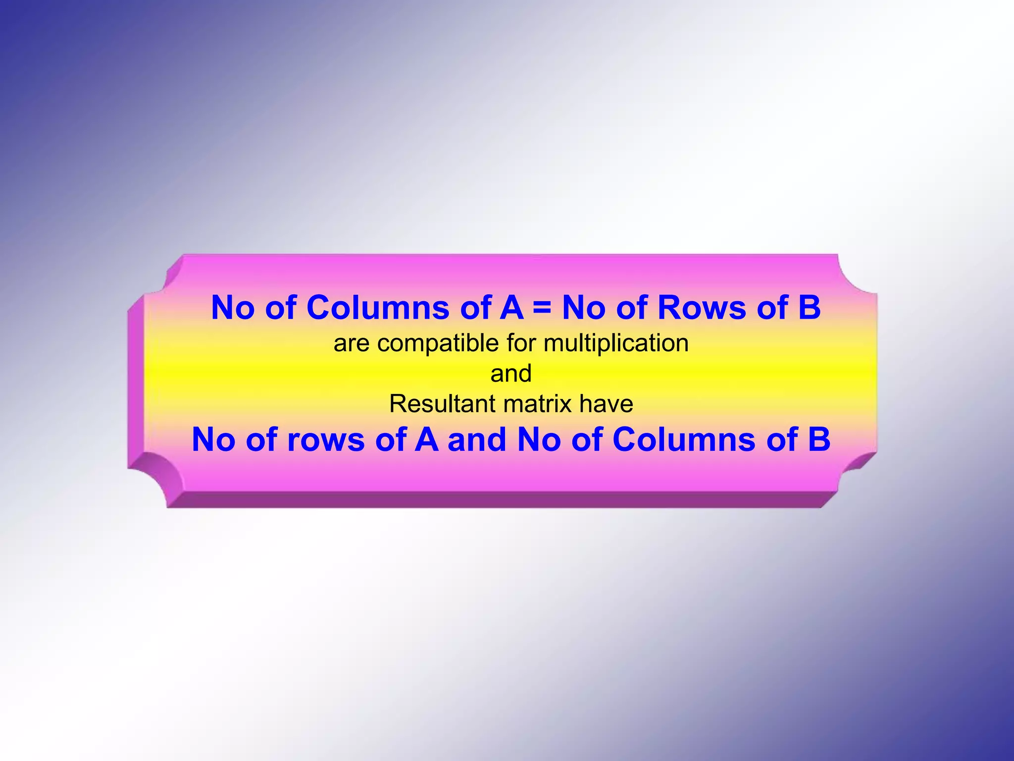
![Product of matrix of A[M x N] and B[M x N] 1. Declare int a[10][10], b[10][10], c[10][10], order of ‘A’ m & n and order of ‘B’ p, q, row index I, column index j and k. 2. Read order of first matrix. cin >> m >> n; 3. Read order of second matrix. cin >> p >> q; 4. If No of columns of A ( n ) != No of Rows of B then terminate the program by giving exit() or return. 3. Repeat for row index I = 0 to m-1 Repeat for Column Index j = 0 to n-1, input value of A [ I ] [ j ] 4. Repeat for row index I = 0 to p-1 Repeat Column Index j = 0 to q-1, input value of B [ I ] [ j ] 5. Repeat for row index I = 0 to m Repeat for column index j = 0 to q C [ I ] [ J ] = 0; Repeat for k = 0 to n C [ I ] [ J ] += A [ I ] [ K ] – B [ K ] [ J ] 6. Print the resultant Matrix C.](https://image.slidesharecdn.com/arrays-200710114741/75/ARRAYS-IN-C-CBSE-AND-STATE-2-COMPUTER-SCIENCE-70-2048.jpg)
![Product of matrix of A[M x N] and B[P x Q] Algorithm 1. For I = 1 to m do 2. { For j = 1 to n do 3. Read A[I, j] } 4. For i = 1 to p do 5. { For j = 1 to q do 6. Read B[I, j] } 7. For I = 1 to m do 8. { for j = 1 to q do 9. { C [ I, J ] = 0 10. For k = 1 to n do 11. C [ I, J] = C [ I, J ] + A [ I, K] * B [ K, J ] } }](https://image.slidesharecdn.com/arrays-200710114741/75/ARRAYS-IN-C-CBSE-AND-STATE-2-COMPUTER-SCIENCE-71-2048.jpg)
![# include <iostream.h> # include <conio.h> # include <iomanip.h> # include <stdlib.h> main() { int a[10][10], b[10][10], c[10][10]; int m, n, p, q, i, j, k; cout << "nEnter the order of 1st Matrix "; cin >> m >> n; cout << "nEnter the order of 2nd Matrix "; cin >> p >> q; if ( n != q) { cout << "nMatrixes can not be Multiply."; getch(); exit(0); } for(i=0; i<m; i++) { cout << "nEnter " << i << "th Row of A "; for(j=0; j<n; j++) cin >> a [ i ] [ j ]; } for(i=0; i<p; i++) { cout << "nEnter " << i << "th Row of B "; for(j=0; j<q; j++) cin >> b [ i ] [ j ]; } for (i=0; i<m; i++) for(j=0; j<q; j++) { c [ i ] [ j ] = 0; for(k=0; k<q; k++) c [ i ] [ j ] += a [ i ] [ k ] * b [ k ] [ j ]; } cout << "nThe Prodect Matrix is "; for(i=0; i<m; i++) { cout << "nn"; for(j=0; j<q; j++) cout << setw(5) << c [ i ] [ j ]; } getch(); } Product of matrix](https://image.slidesharecdn.com/arrays-200710114741/75/ARRAYS-IN-C-CBSE-AND-STATE-2-COMPUTER-SCIENCE-73-2048.jpg)
![Matrix A Col 0 Col 1 Col 2 Row 0 1 2 3 Row 1 4 5 6 Row 2 7 8 9 Matrix C Col 0 Col 1 Col 2 Row 0 1 4 7 Row 1 2 5 8 Row 2 3 6 9 C [ i ] [ j ] = A [ j ] [ i ] Show 1 For Row index I = 0 to 2 { For Column index J = 0 to 2 { C [ I ] [ J ] = A [ J ] [ I ] } } Transpose of a Matrix. If we interchange the rows and columns of a matrix, then this new matrix is known as the transpose of the given matrix. C [ 0 ] [ 0 ] = A [ 0 ] [ 0 ] C [ 0 ] [ 1 ] = A [ 1 ] [ 0 ] C [ 0 ] [ 2 ] = A [ 2 ] [ 0 ] C [ 1 ] [ 0 ] = A [ 0 ] [ 1 ] C [ 1 ] [ 1 ] = A [ 1 ] [ 1 ] C [ 1 ] [ 2 ] = A [ 2 ] [ 1 ] C [ 2 ] [ 0 ] = A [ 0 ] [ 2 ] C [ 2 ] [ 1 ] = A [ 1 ] [ 2 ] C [ 2 ] [ 2 ] = A [ 2 ] [ 2 ] 2 3 4 5 6 7 8 9](https://image.slidesharecdn.com/arrays-200710114741/75/ARRAYS-IN-C-CBSE-AND-STATE-2-COMPUTER-SCIENCE-74-2048.jpg)
![Transpose of matrix of A[M x N] and B[M x N] 1. Declare int a[10][10], b[10][10], order of matrix m & n and row index I, column index j. 2. Read order of matrix. cin >> m >> n; 3. Repeat for row index I = 0 to m-1 Repeat for Column Index j = 0 to n-1, input value of A [ I ] [ j ] 4. Repeat for row index I = 0 to p-1 Repeat for Column Index j = 0 to q-1 B [ I ] [ j ] = C [ J ] [ I ] 5. Repeat for row index I = 0 to N Print “nn” Repeat for column index j = 0 to M Print B [ I ] [ J ]](https://image.slidesharecdn.com/arrays-200710114741/75/ARRAYS-IN-C-CBSE-AND-STATE-2-COMPUTER-SCIENCE-75-2048.jpg)
![# include <iostream.h> # include <conio.h> # include <iomanip.h> main() { int a[10][10], b[10][10], m, n, i, j; clrscr(); cout << "nnEnter the order of Matrix "; cin >> m >> n; for(i=0; i<m; i++) { cout << "nEnter " << i << "th Row "; for(j=0; j<n; j++) cin >> a [ i ] [ j ]; } for (i=0; i<m; i++) for(j=0; j<n; j++) { b [ i ] [ j ] = a [ j ] [ i ]; } cout << "nnThe Transpose of Matrix is "; for(i=0; i<n; i++) { cout << "nn"; for(j=0; j<m; j++) cout << setw(5) << b [ i ] [ j ]; } getch(); } C [ i ] [ j ] = A [ j ] [ i ] Transpose of matrix](https://image.slidesharecdn.com/arrays-200710114741/75/ARRAYS-IN-C-CBSE-AND-STATE-2-COMPUTER-SCIENCE-76-2048.jpg)
![# include <iostream.h> # include <conio.h> # include <iomanip.h> main() { int a[10][10], b[10][10], m, n, i, j, k; cout << "nnEnter the order of Matrix "; cin >> m >> n; for(i=0; i<m; i++) { cout << "nnPls Enter " << i << "th Row of A "; for(j=0; j<n; j++) cin >> a [ i ] [ j ]; } cout << "nnEnter the value of k. "; cin >> k; for (i=0; i<m; i++) for(j=0; j<n; j++) { b [ i ] [ j ] = a [ i ] [ j ] * k; } cout << "nnThe k x A Matrix is "; for(i=0; i<n; i++) { cout << "nn"; for(j=0; j<m; j++) cout << setw(5) << b[i][j]; } getch(); } Each element in the Array will be multiplied by ‘k’ and assign it in the second array ‘b’. b [ i ] [ j ] = A [ i ] [ j ] * k k x Matrix A An integer Value](https://image.slidesharecdn.com/arrays-200710114741/75/ARRAYS-IN-C-CBSE-AND-STATE-2-COMPUTER-SCIENCE-77-2048.jpg)


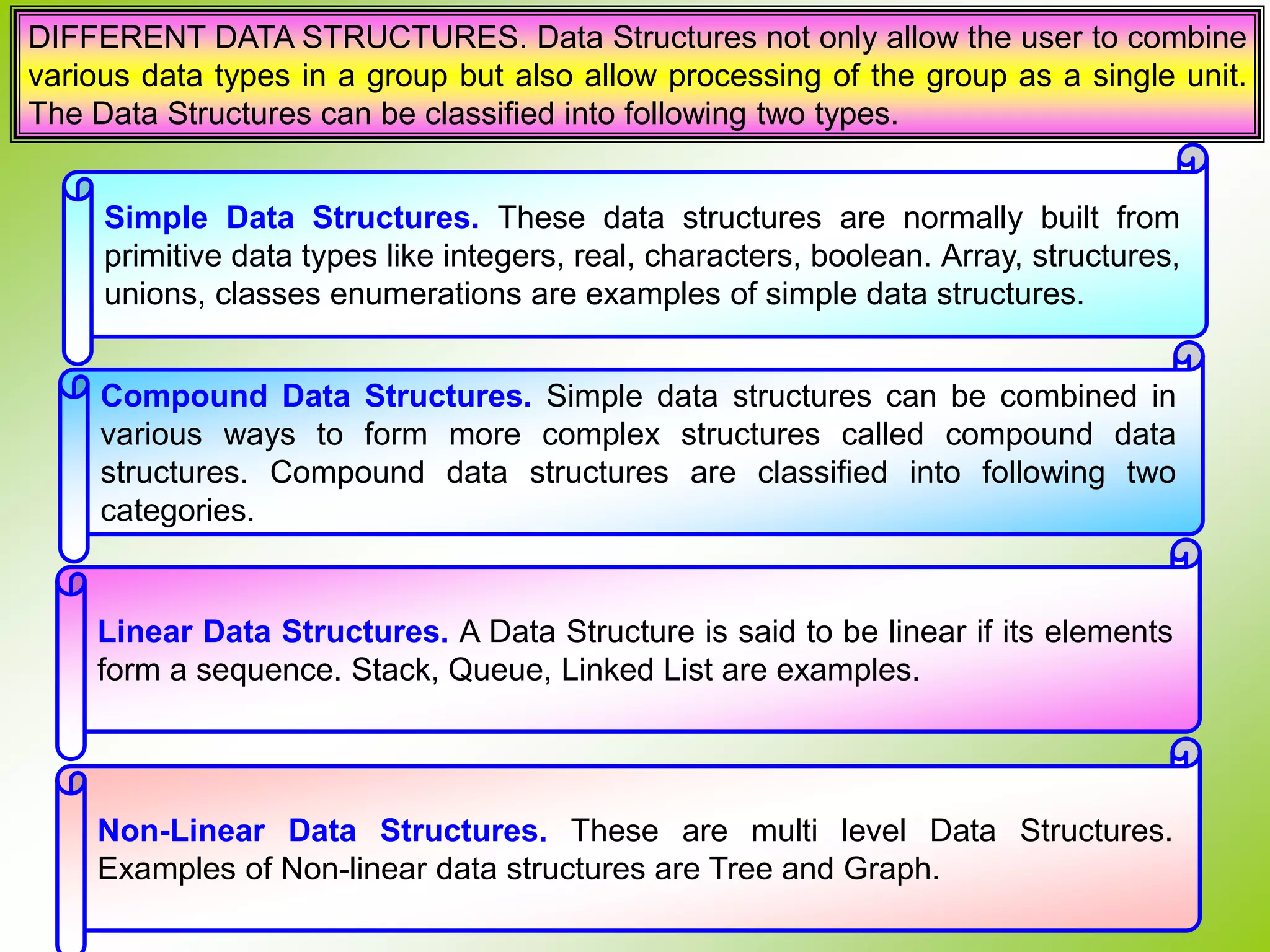
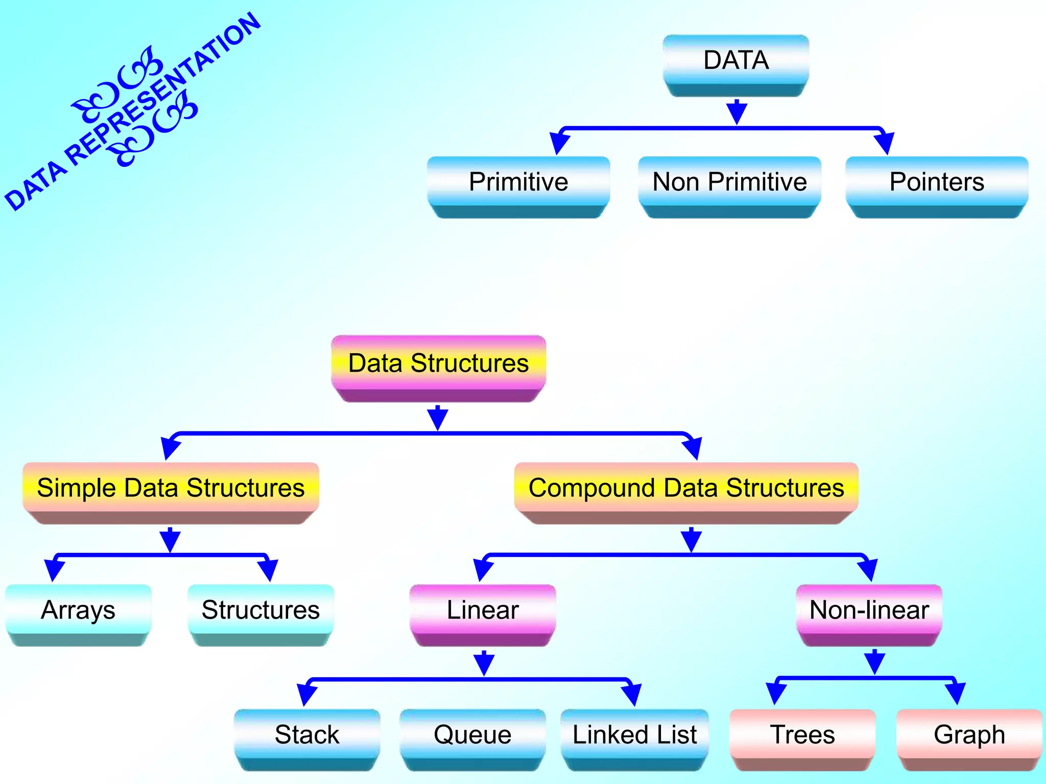
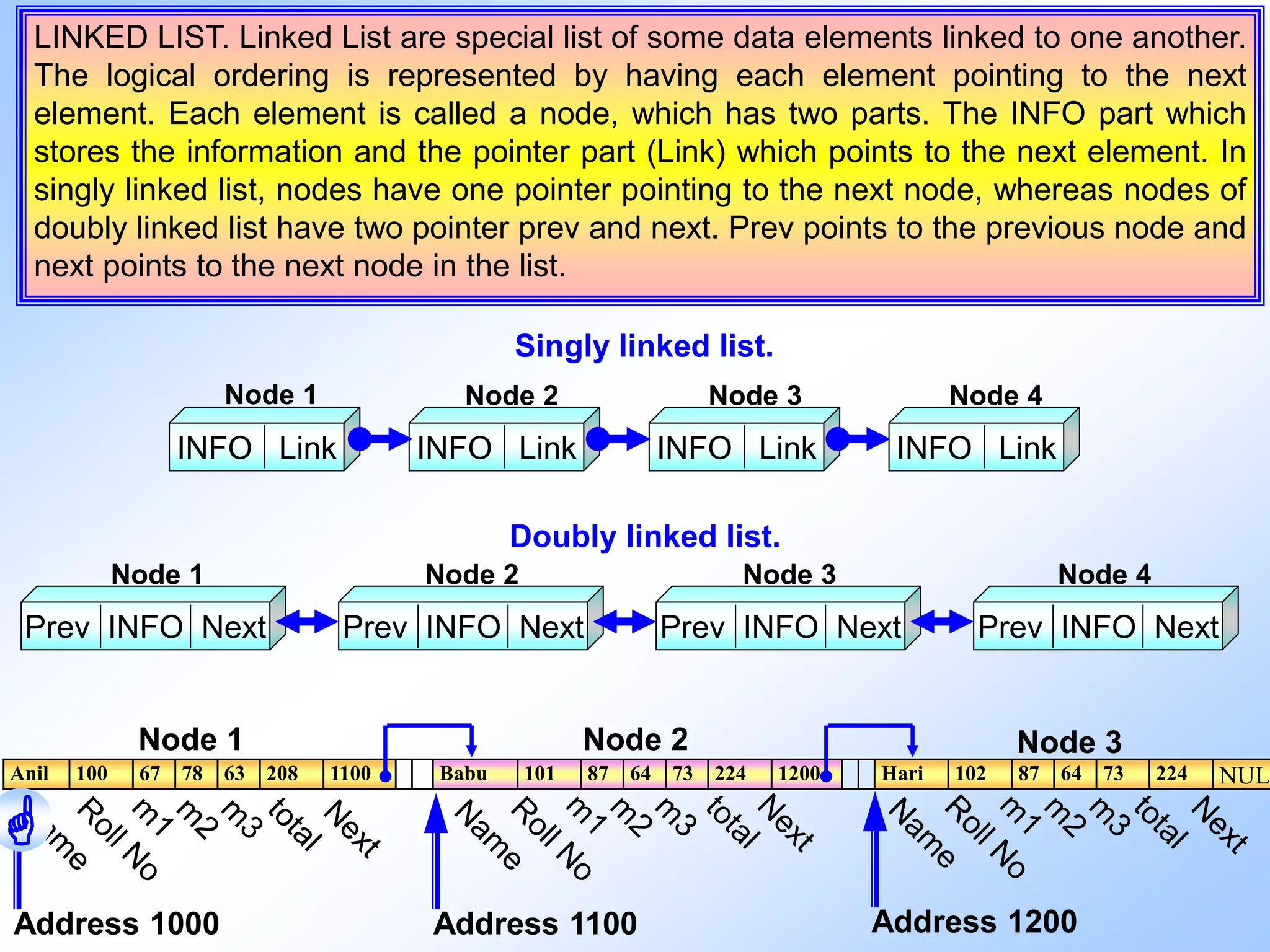
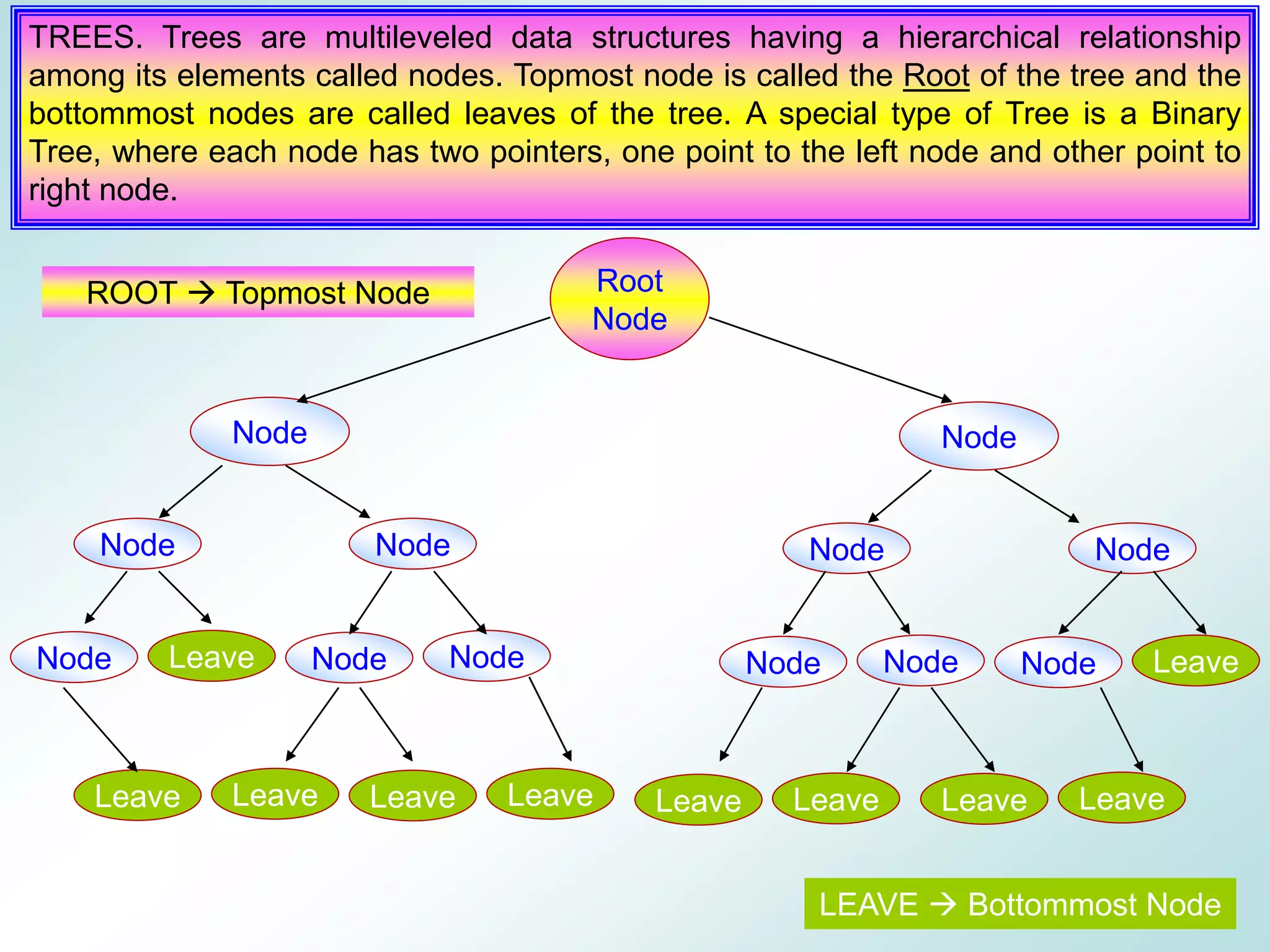
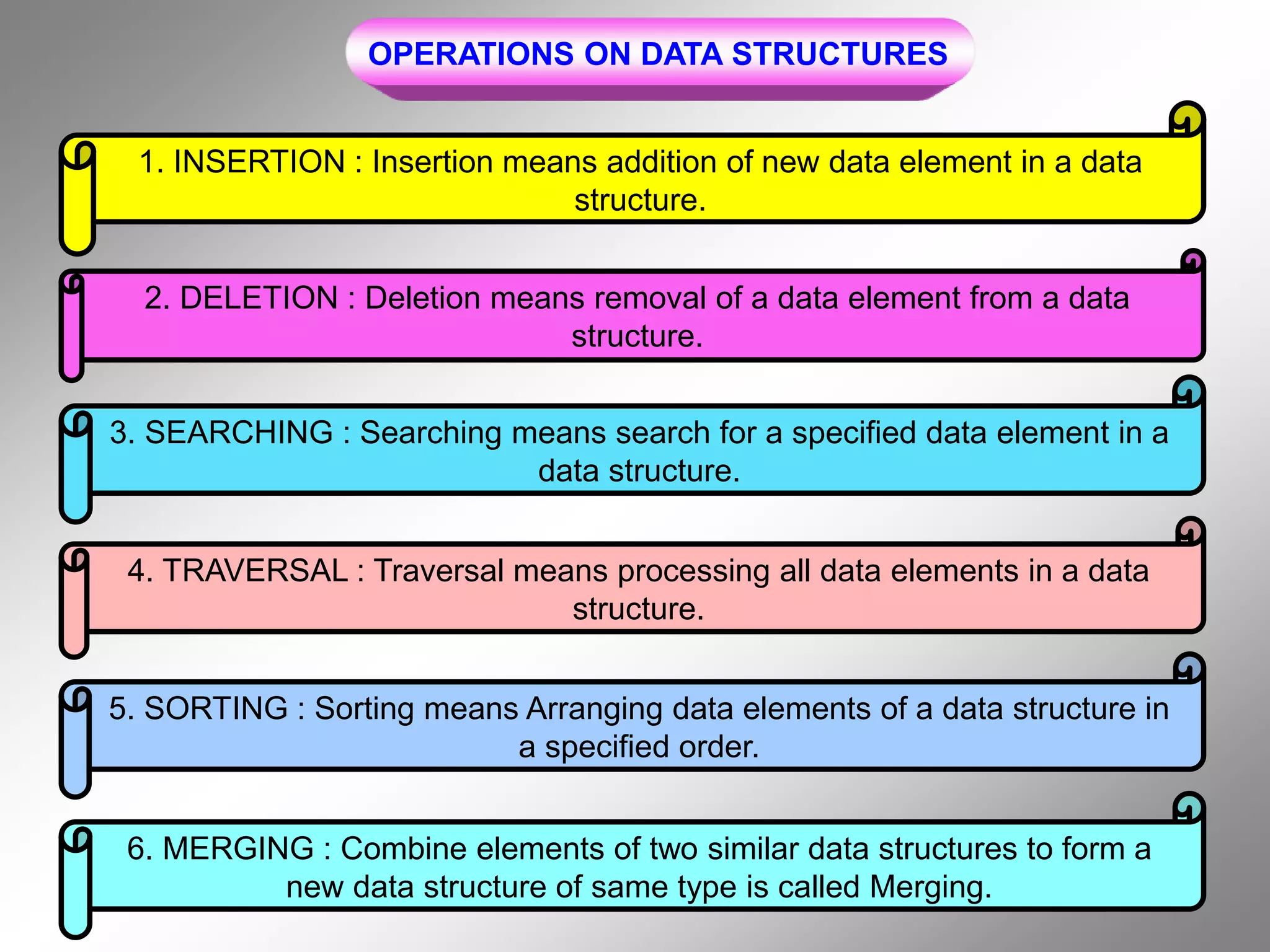
The document discusses different data types and data structures. It begins by defining raw data, data items, and data structures. It then describes primitive and non-primitive data types, including integers, reals, characters, arrays, structures, classes and unions. The document also covers different data structures like arrays, stacks, queues, linked lists and trees. It explains how each data structure stores and organizes data and describes common operations like insertion, deletion, searching, traversal and sorting.