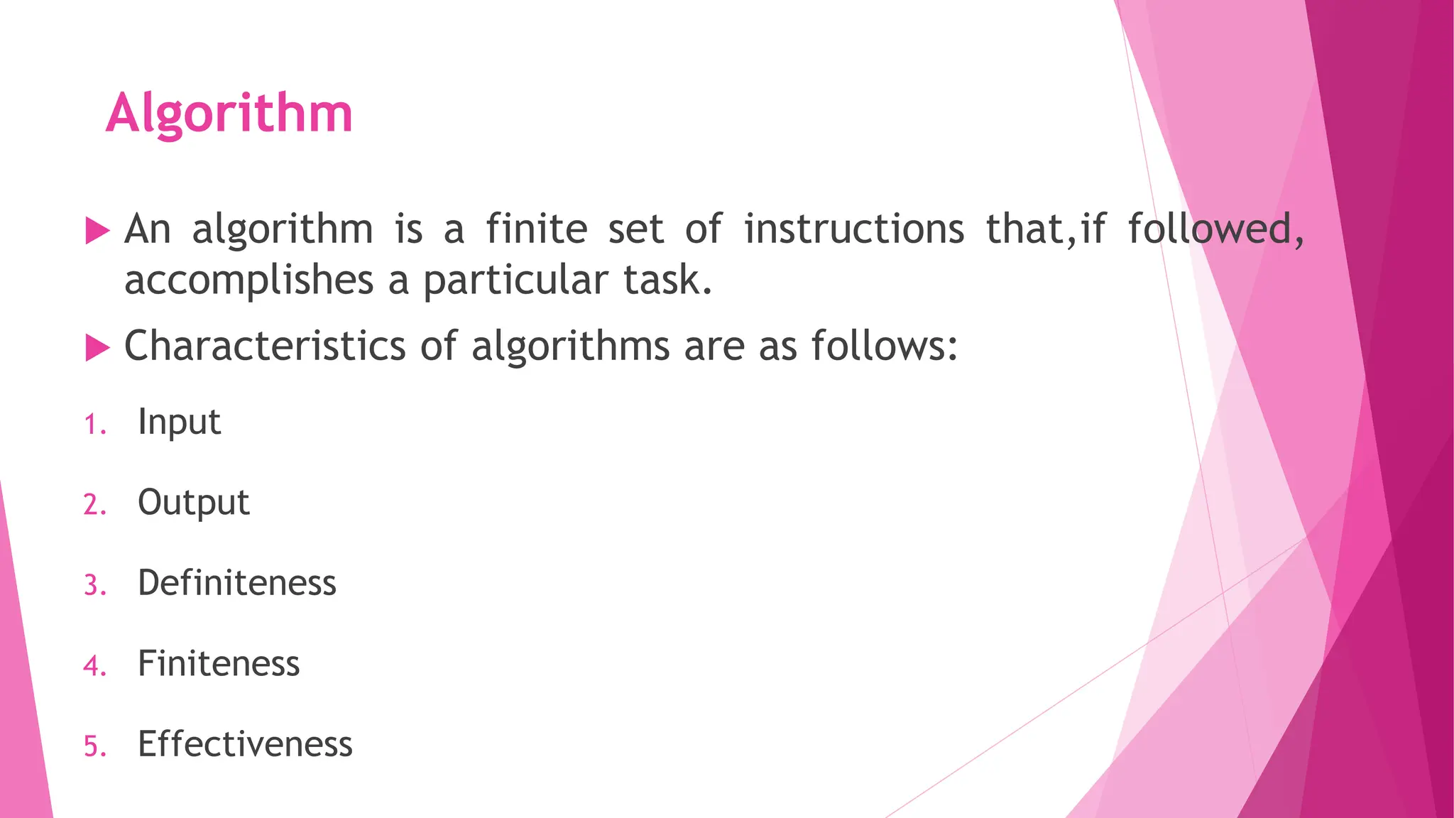
The document outlines the essential characteristics of algorithms, including inputs, outputs, definiteness, finiteness, and effectiveness. It discusses pseudocode conventions, recursive algorithms, and performance analysis focusing on time and space complexity, while also introducing asymptotic notations for evaluating algorithm efficiency. Various methods for solving recurrences and examples demonstrating these concepts are also provided.

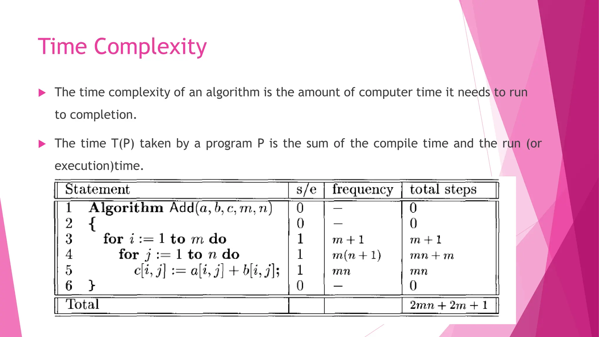
![Performance Analysis Aim of this course is to develop skills for making evaluative judgments about algorithm. There are two criteria for judging algorithms that have a more direct relationship to performance. These have to do with their computing time and storage requirements. [Space/Time complexity] The space complexity of an algorithm is the amount of memory it needs to run to completion. The time complexity of an algorithm is the amount of computer time it needs to run to completion Performance evaluation can be loosely divided into two major phases: (1) a priori estimates and (2) a posteriori testing. We refer to these as performance analysis and performance measurement respectively.](https://image.slidesharecdn.com/analysisofalgorithms1-240611062926-ee3f3756/75/Analysis-of-Algorithms-recurrence-relation-solving-recurrences-7-2048.jpg)