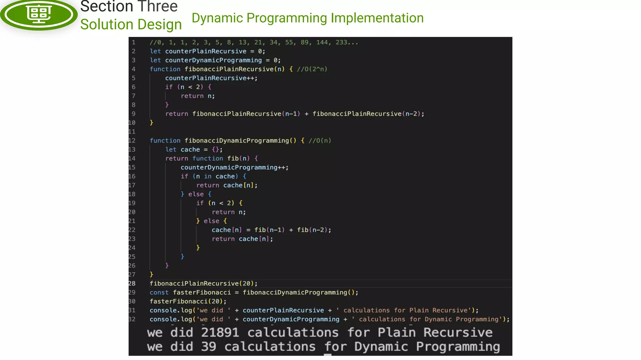
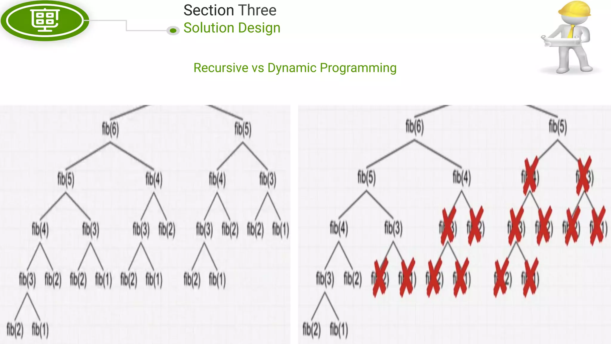
Software Architect Algorithm Analysis & Design Big-O and Solution Design
by Douglas Crockford
- Principal Software Architect at Telkom Indonesia - Engineering Lead of Digital Product Engineering Chapter Digital Business & Technology - Solutions Architect at Online Single Submission System (oss.go.id) - Head of Engineer at Peduli Lindungi - Software Architect Lead at Telkom Indonesia - Professional Mentor at Purwadhika Digital Technology School - Cloud Computing Instructor at Google Bangkit - Software Engineer - Professional Lecture - Researcher - Speaker - Author Rony Setyawan, S.T., M.Kom., CCP., CSAP.
by Grady Booch
Type of Big-O Big-O Rules Solution Design Q&A
Easy to Maintain (Readability) Easy to Scale (Scalability) Good or Bad Code? Section One Theory and Practice of Big-O
Section One Theory and Practice of Big-O Big-O Complexity Chart
Section One Theory and Practice of Big-O Experiment 1
Section One Theory and Practice of Big-O Experiment 2
Section One Theory and Practice of Big-O Experiment 3
Section One Theory and Practice of Big-O Conclusion Experiment 1, 2, 3 The increase in the amount of data (elements) will be directly proportional to the increase in the time needed to run the task (number of operations needed). Within Big O, the main topic of discussion is how do we make our algorithm as good as possible in the Excellent, Good, or Fair area. And we need to avoid Horrible and Bad areas. So, this is not a contradiction with Conclusion 1. An algorithm is said to be Scalable, if the algorithm is O(log n), O(1), or O(n). Apart from doing some refactoring so that we can enter into one of those areas of Big O notation. In experiments 1, 2, and 3, the function is in O(n).
Section One Theory and Practice of Big-O Linear Time Big-O For Loop While Loop What kind of implementation?
Section One Theory and Practice of Big-O Experiment 4
Section One Theory and Practice of Big-O Experiment 5
Section One Theory and Practice of Big-O Experiment 6
Section One Theory and Practice of Big-O Conclusion Experiment 4, 5, 6 The amount of data we use has no effect at all on the performance of the function Time is always constant (fixed) even though the amount of data changes whether it's getting smaller or bigger In experiments 4, 5, and 6, the function is in O(1).
Section One Theory and Practice of Big-O Constant Time Big-O All Single Statement No Loop Function What kind of implementation?
Section One Theory and Practice of Big-O Big-O Calculation Example
Section One Theory and Practice of Big-O Experiment 7
Section One Theory and Practice of Big-O Conclusion Experiment 7 Nested Loop (marked by an indentation) it means that it indicates multiplication (*) not Addition (+) The number of menus generated is 16 menus, this is obtained from multiplication (foods, drinks) In experiments 7, the function is in O(n^2).
Section One Theory and Practice of Big-O Nested For Loop Nested While Loop What kind of implementation? Nested Loop Quadratic Time Big-O
Section One Theory and Practice of Big-O Experiment 8 Problem Statement: ● There are several candidates for the presidential candidates for Indonesia in 2024. ● They will be scheduled to debate the presidential candidates and take serial numbers for their identities later during the campaign. ● At the meeting, of course, several chairs are needed to be used by these candidates, then how can we arrange these chairs? ● Please provide an alternative to the seat arrangement for the three presidential candidates!
Section One Theory and Practice of Big-O Experiment 9
Section One Theory and Practice of Big-O Result Experiment 9
Section One Theory and Practice of Big-O Conclusion Experiment 8 and 9 When we use 3 input data, it produces 6 output data (3! = 6) When we use 4 input data, it produces 24 output data (4! = 24) The exact number of operations required will of course depend on the algorithm used In experiment 8 & 9, use the recursive function approach. In experiments 8 and 9, the function is in O(n!) or Factorial Big-O.
Section Two Big-O Rules Experiment 10
Section Two Big-O Rules Big O Rule 1 : Worst Case Scenario is the most we care about / Drop non-dominant terms Big O Rule 1 states that we cannot always expect ideal conditions such as for example ideal input on the contrary we need to pay attention to conditions that are not ideal so that our program runs in the most inefficient state. Therefore, in Experiment 10 we can say that the function belongs to O(n). Experiment 10 ● Input 'Telkom' (0), so it only requires 1 search process ● Input 'AT&T' (4), so it only takes 5 searching processes ● Input 'T-Mobile' (10), then it requires 11 searching processes
Section Two Big-O Rules Experiment 11 Problem Statement: ● The marketing and product teams have customer data totaling 100 mobile numbers. ● Approaching the end of the year, there is an initiative to send promos to all customers using existing mobile number data. ● Apart from the promo, there is also a special discount given to only 10 customers selected by the product team.
Section Two Big-O Rules Result Experiment 11 Big O Rule 2 : Remove Every Constants Let's take a closer look at Experiment 11, specifically for the SendPromoDiscount function. In Big O calculations for this function actually consists of O(n) and O(10). Simplify it then becomes O(n + 10). Big O Rule 2 states that We Must Remove Every Constant, then ignore the O(10). Compared to O(n), which is not fixed and can have a very large impact.
Section Two Big-O Rules Experiment 12
Section Two Big-O Rules Experiment 13
Section Two Big-O Rules Experiment 12 and 13 ● Based on Big O Rule 1, we can ignore the existing O(2). ● Based on Big O Rule 2, in Experiment 12 we can ignore the existing Contacts. So, we can simplify O(2n) to only O(n). ● Based on Big O Rule 3, we cannot simplify Experiment 13 so that the Big O notation we get is O(m + n). Big O Rule 3 : Different Terms for Inputs Big O Rule 3 states that if we find a function/program that uses different input data, then we can not simplify Big O notation because different input data can significantly affect the complexity or number of operations required.
Section Two Big-O Rules Time Complexity of Big-O
Section Three Solution Design Hash Table https://www.miraclesalad.com/webtools/md5.php https://www.cs.usfca.edu/~galles/visualization/OpenHash.html Hash table, also known as hash map, is a data structure that implements an associative array or dictionary. It is an abstract data type that maps keys to values. A hash table uses a hash function to compute an index, also called a hash code, into an array of buckets or slots, from which the desired value can be found. During lookup, the key is hashed and the resulting hash indicates where the corresponding value is stored. Hash Function Simulation
Section Three Solution Design Hash Table
Section Three Solution Design Hash Tables Overview
Section Three Solution Design Arrays vs Hash Tables
Hash Tables Implementation Section Three Solution Design
Section Three Solution Design Dynamic Programming Can be divided into subproblems Commonly based on plain recursive solution Are there repetitive subproblems Memoize subproblems
Dynamic Programming Implementation Section Three Solution Design
Section Three Solution Design Recursive vs Dynamic Programming
Any Question?
by Bertrand Meyer
THANK YOU

Algorithm Analysis & Solution Design.pdf

  • 1.
    Software Architect Algorithm Analysis &Design Big-O and Solution Design
  • 2.
  • 3.
    - Principal SoftwareArchitect at Telkom Indonesia - Engineering Lead of Digital Product Engineering Chapter Digital Business & Technology - Solutions Architect at Online Single Submission System (oss.go.id) - Head of Engineer at Peduli Lindungi - Software Architect Lead at Telkom Indonesia - Professional Mentor at Purwadhika Digital Technology School - Cloud Computing Instructor at Google Bangkit - Software Engineer - Professional Lecture - Researcher - Speaker - Author Rony Setyawan, S.T., M.Kom., CCP., CSAP.
  • 4.
  • 5.
    Type of Big-OBig-O Rules Solution Design Q&A
  • 6.
    Easy to Maintain(Readability) Easy to Scale (Scalability) Good or Bad Code? Section One Theory and Practice of Big-O
  • 7.
    Section One Theory andPractice of Big-O Big-O Complexity Chart
  • 8.
    Section One Theory andPractice of Big-O Experiment 1
  • 9.
    Section One Theory andPractice of Big-O Experiment 2
  • 10.
    Section One Theory andPractice of Big-O Experiment 3
  • 11.
    Section One Theory andPractice of Big-O Conclusion Experiment 1, 2, 3 The increase in the amount of data (elements) will be directly proportional to the increase in the time needed to run the task (number of operations needed). Within Big O, the main topic of discussion is how do we make our algorithm as good as possible in the Excellent, Good, or Fair area. And we need to avoid Horrible and Bad areas. So, this is not a contradiction with Conclusion 1. An algorithm is said to be Scalable, if the algorithm is O(log n), O(1), or O(n). Apart from doing some refactoring so that we can enter into one of those areas of Big O notation. In experiments 1, 2, and 3, the function is in O(n).
  • 12.
    Section One Theory andPractice of Big-O Linear Time Big-O For Loop While Loop What kind of implementation?
  • 13.
    Section One Theory andPractice of Big-O Experiment 4
  • 14.
    Section One Theory andPractice of Big-O Experiment 5
  • 15.
    Section One Theory andPractice of Big-O Experiment 6
  • 16.
    Section One Theory andPractice of Big-O Conclusion Experiment 4, 5, 6 The amount of data we use has no effect at all on the performance of the function Time is always constant (fixed) even though the amount of data changes whether it's getting smaller or bigger In experiments 4, 5, and 6, the function is in O(1).
  • 17.
    Section One Theory andPractice of Big-O Constant Time Big-O All Single Statement No Loop Function What kind of implementation?
  • 18.
    Section One Theory andPractice of Big-O Big-O Calculation Example
  • 19.
    Section One Theory andPractice of Big-O Experiment 7
  • 20.
    Section One Theory andPractice of Big-O Conclusion Experiment 7 Nested Loop (marked by an indentation) it means that it indicates multiplication (*) not Addition (+) The number of menus generated is 16 menus, this is obtained from multiplication (foods, drinks) In experiments 7, the function is in O(n^2).
  • 21.
    Section One Theory andPractice of Big-O Nested For Loop Nested While Loop What kind of implementation? Nested Loop Quadratic Time Big-O
  • 22.
    Section One Theory andPractice of Big-O Experiment 8 Problem Statement: ● There are several candidates for the presidential candidates for Indonesia in 2024. ● They will be scheduled to debate the presidential candidates and take serial numbers for their identities later during the campaign. ● At the meeting, of course, several chairs are needed to be used by these candidates, then how can we arrange these chairs? ● Please provide an alternative to the seat arrangement for the three presidential candidates!
  • 23.
    Section One Theory andPractice of Big-O Experiment 9
  • 24.
    Section One Theory andPractice of Big-O Result Experiment 9
  • 25.
    Section One Theory andPractice of Big-O Conclusion Experiment 8 and 9 When we use 3 input data, it produces 6 output data (3! = 6) When we use 4 input data, it produces 24 output data (4! = 24) The exact number of operations required will of course depend on the algorithm used In experiment 8 & 9, use the recursive function approach. In experiments 8 and 9, the function is in O(n!) or Factorial Big-O.
  • 26.
  • 27.
    Section Two Big-O Rules BigO Rule 1 : Worst Case Scenario is the most we care about / Drop non-dominant terms Big O Rule 1 states that we cannot always expect ideal conditions such as for example ideal input on the contrary we need to pay attention to conditions that are not ideal so that our program runs in the most inefficient state. Therefore, in Experiment 10 we can say that the function belongs to O(n). Experiment 10 ● Input 'Telkom' (0), so it only requires 1 search process ● Input 'AT&T' (4), so it only takes 5 searching processes ● Input 'T-Mobile' (10), then it requires 11 searching processes
  • 28.
    Section Two Big-O Rules Experiment11 Problem Statement: ● The marketing and product teams have customer data totaling 100 mobile numbers. ● Approaching the end of the year, there is an initiative to send promos to all customers using existing mobile number data. ● Apart from the promo, there is also a special discount given to only 10 customers selected by the product team.
  • 29.
    Section Two Big-O Rules ResultExperiment 11 Big O Rule 2 : Remove Every Constants Let's take a closer look at Experiment 11, specifically for the SendPromoDiscount function. In Big O calculations for this function actually consists of O(n) and O(10). Simplify it then becomes O(n + 10). Big O Rule 2 states that We Must Remove Every Constant, then ignore the O(10). Compared to O(n), which is not fixed and can have a very large impact.
  • 30.
  • 31.
  • 32.
    Section Two Big-O Rules Experiment12 and 13 ● Based on Big O Rule 1, we can ignore the existing O(2). ● Based on Big O Rule 2, in Experiment 12 we can ignore the existing Contacts. So, we can simplify O(2n) to only O(n). ● Based on Big O Rule 3, we cannot simplify Experiment 13 so that the Big O notation we get is O(m + n). Big O Rule 3 : Different Terms for Inputs Big O Rule 3 states that if we find a function/program that uses different input data, then we can not simplify Big O notation because different input data can significantly affect the complexity or number of operations required.
  • 33.
    Section Two Big-O Rules TimeComplexity of Big-O
  • 34.
    Section Three Solution Design HashTable https://www.miraclesalad.com/webtools/md5.php https://www.cs.usfca.edu/~galles/visualization/OpenHash.html Hash table, also known as hash map, is a data structure that implements an associative array or dictionary. It is an abstract data type that maps keys to values. A hash table uses a hash function to compute an index, also called a hash code, into an array of buckets or slots, from which the desired value can be found. During lookup, the key is hashed and the resulting hash indicates where the corresponding value is stored. Hash Function Simulation
  • 35.
  • 36.
  • 37.
  • 38.
  • 39.
    Section Three Solution Design DynamicProgramming Can be divided into subproblems Commonly based on plain recursive solution Are there repetitive subproblems Memoize subproblems
  • 40.
  • 41.
  • 42.
  • 43.
  • 44.