Algo complexity

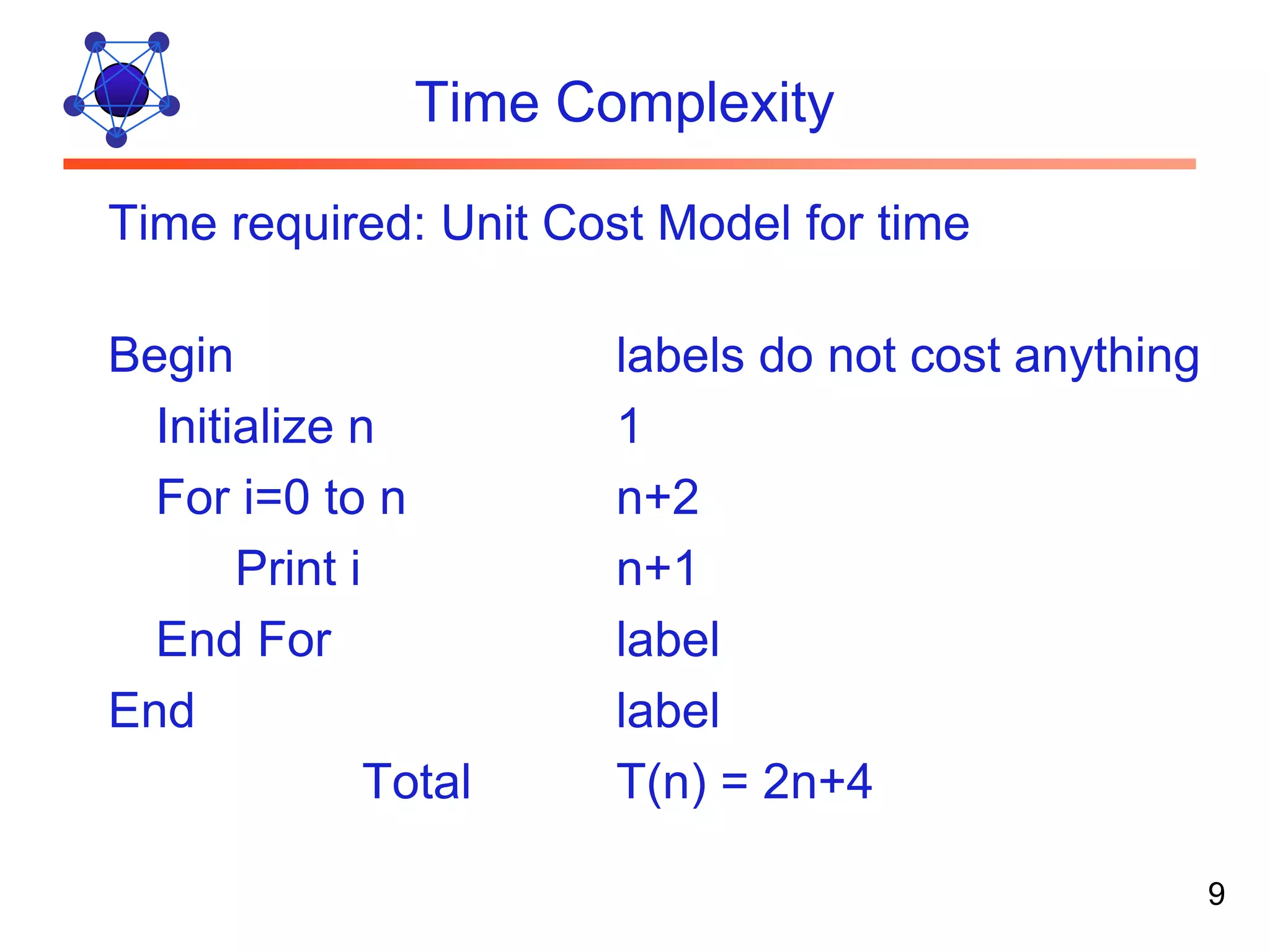
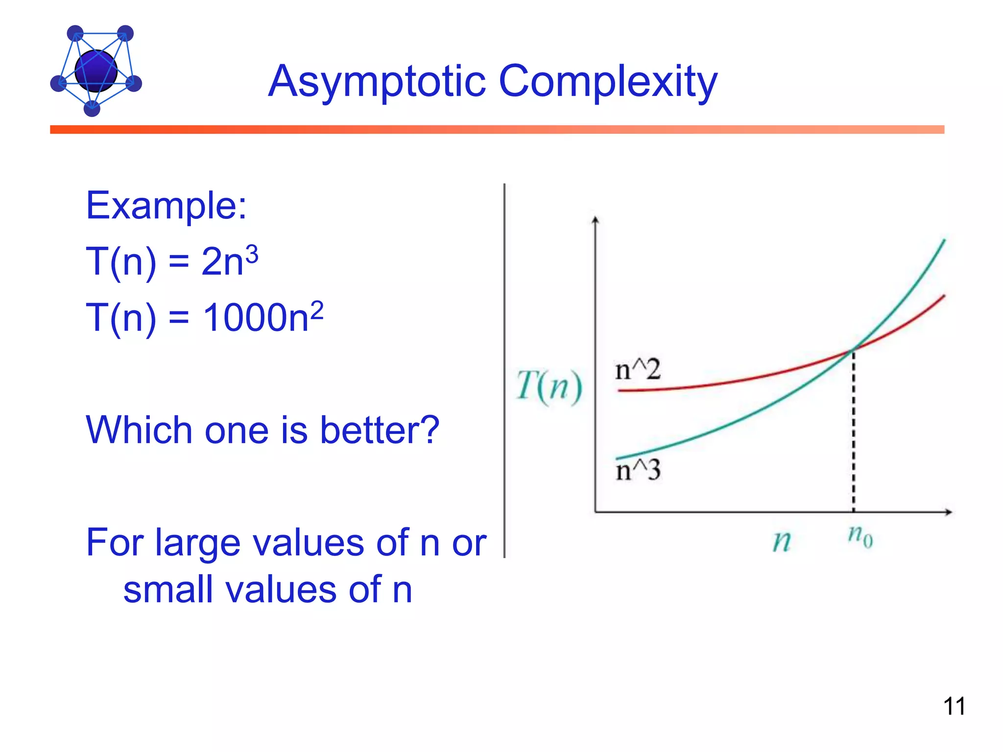
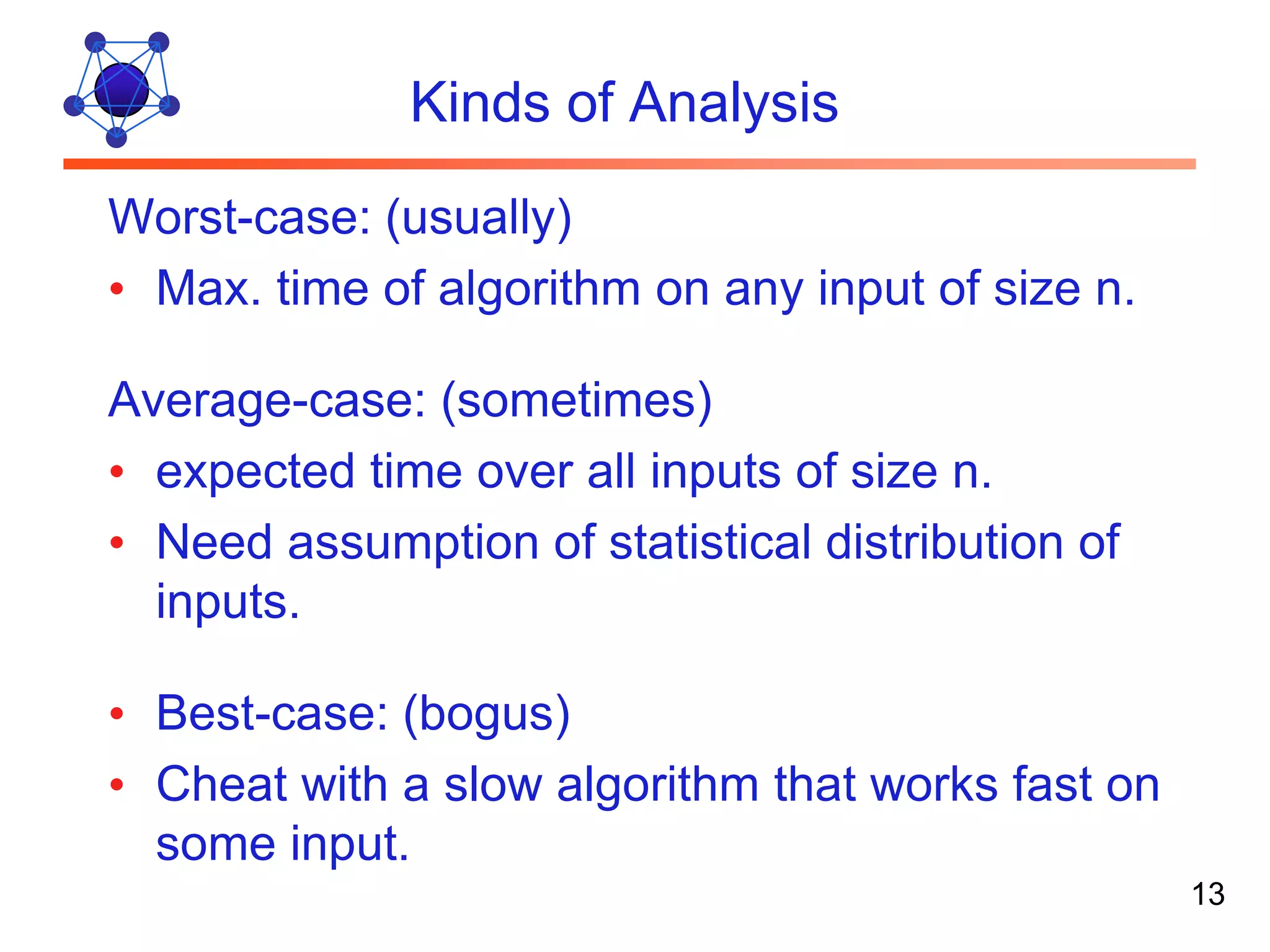
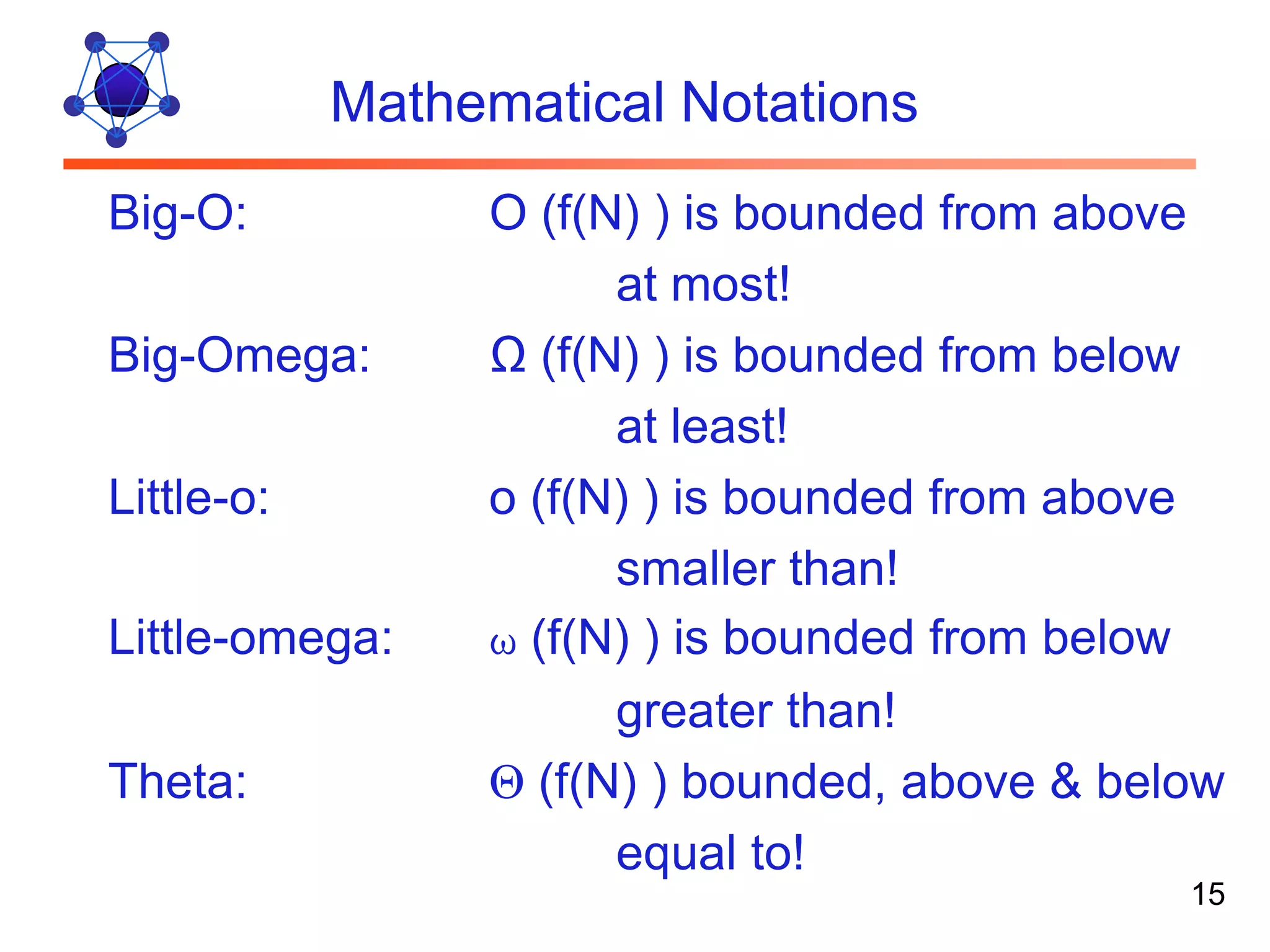
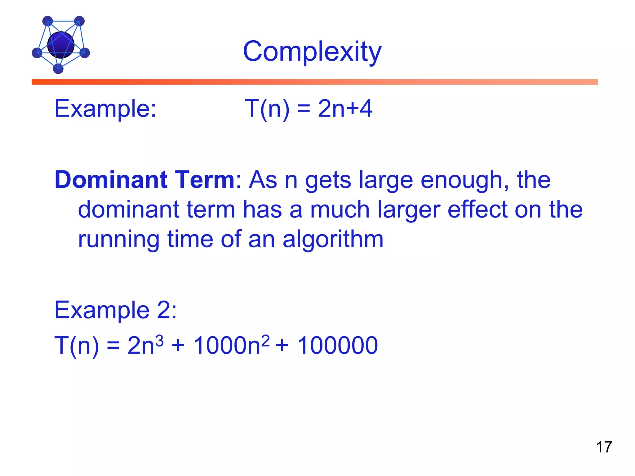
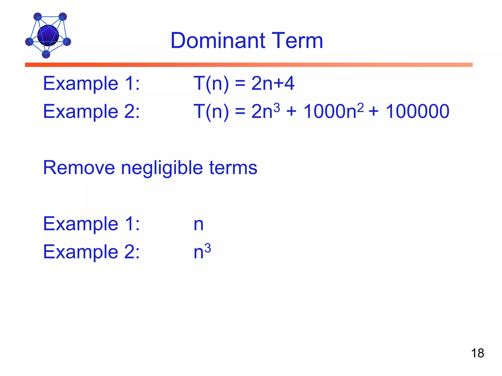
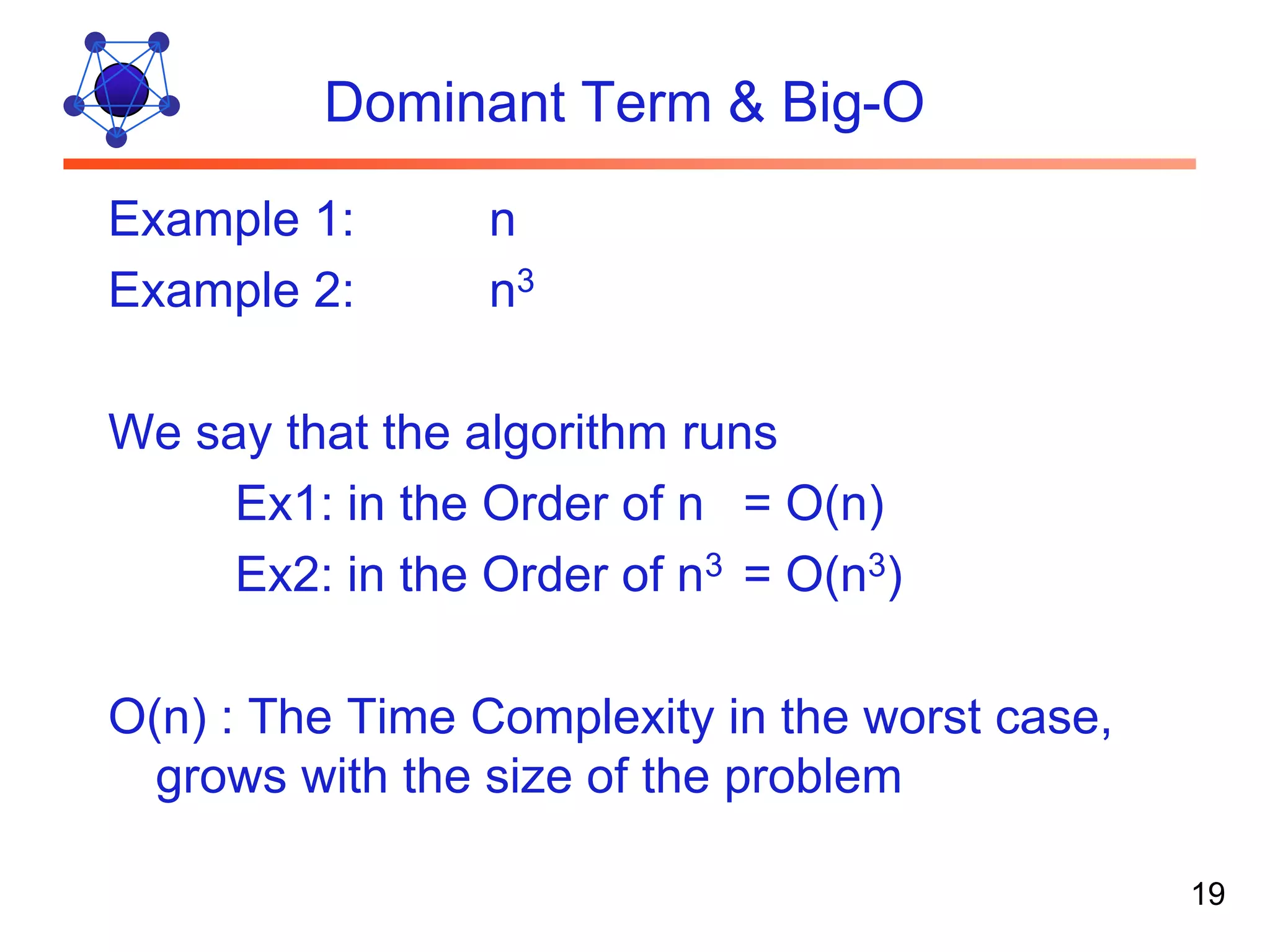
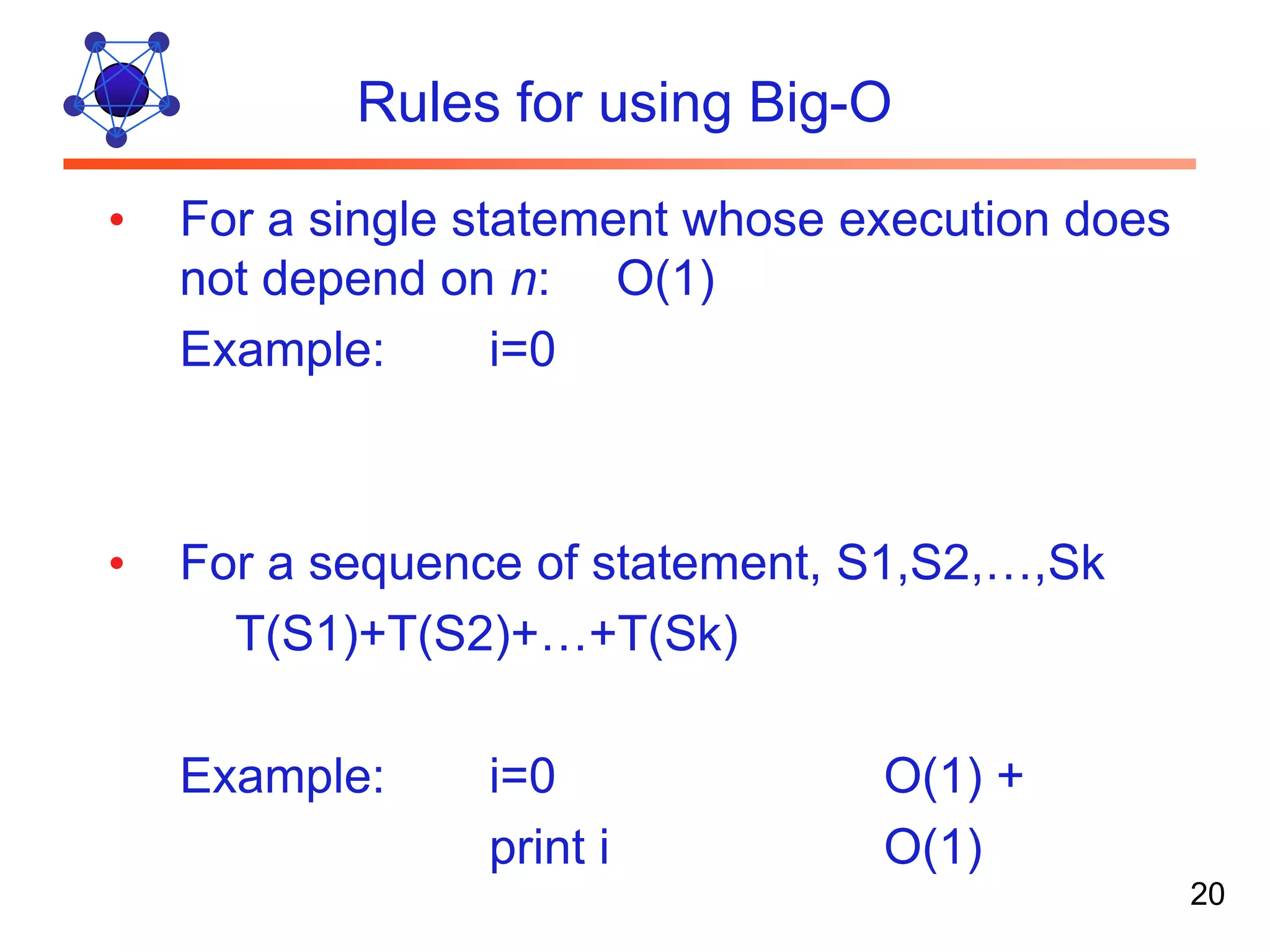
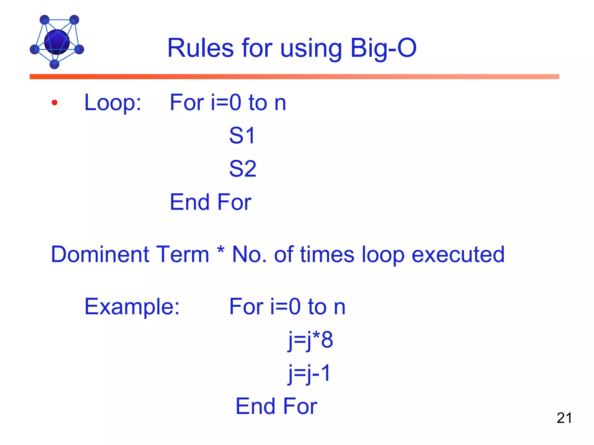
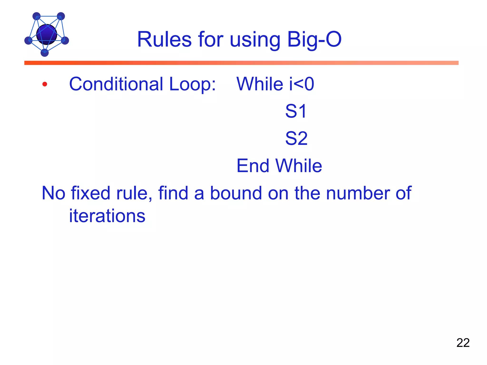
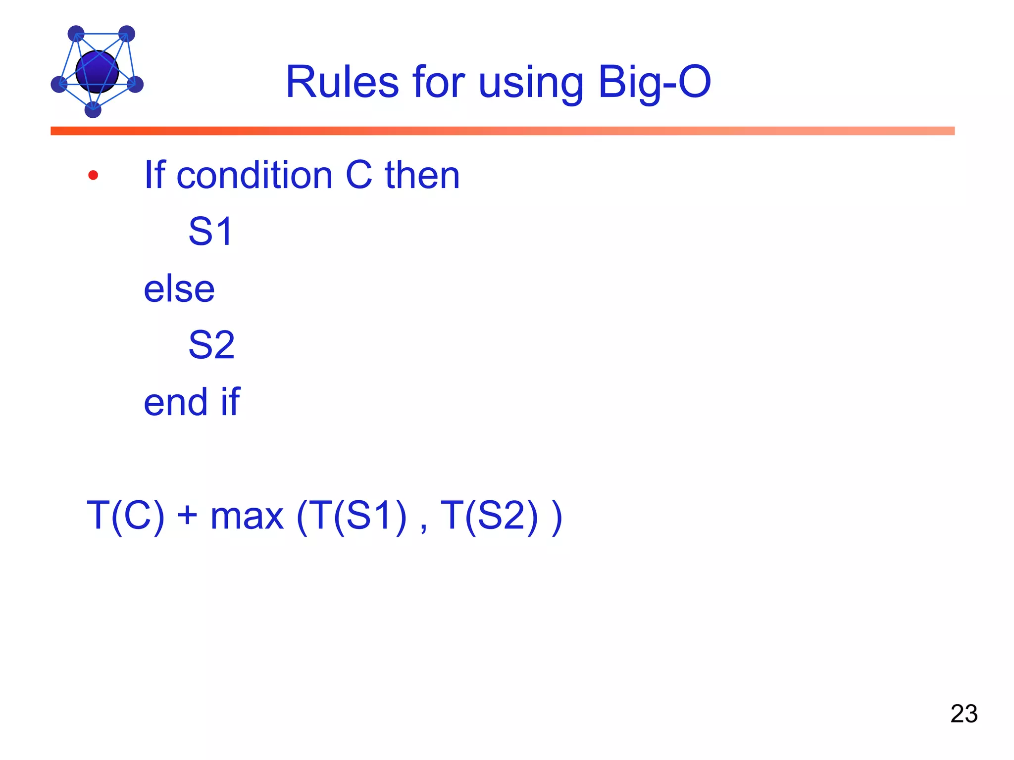
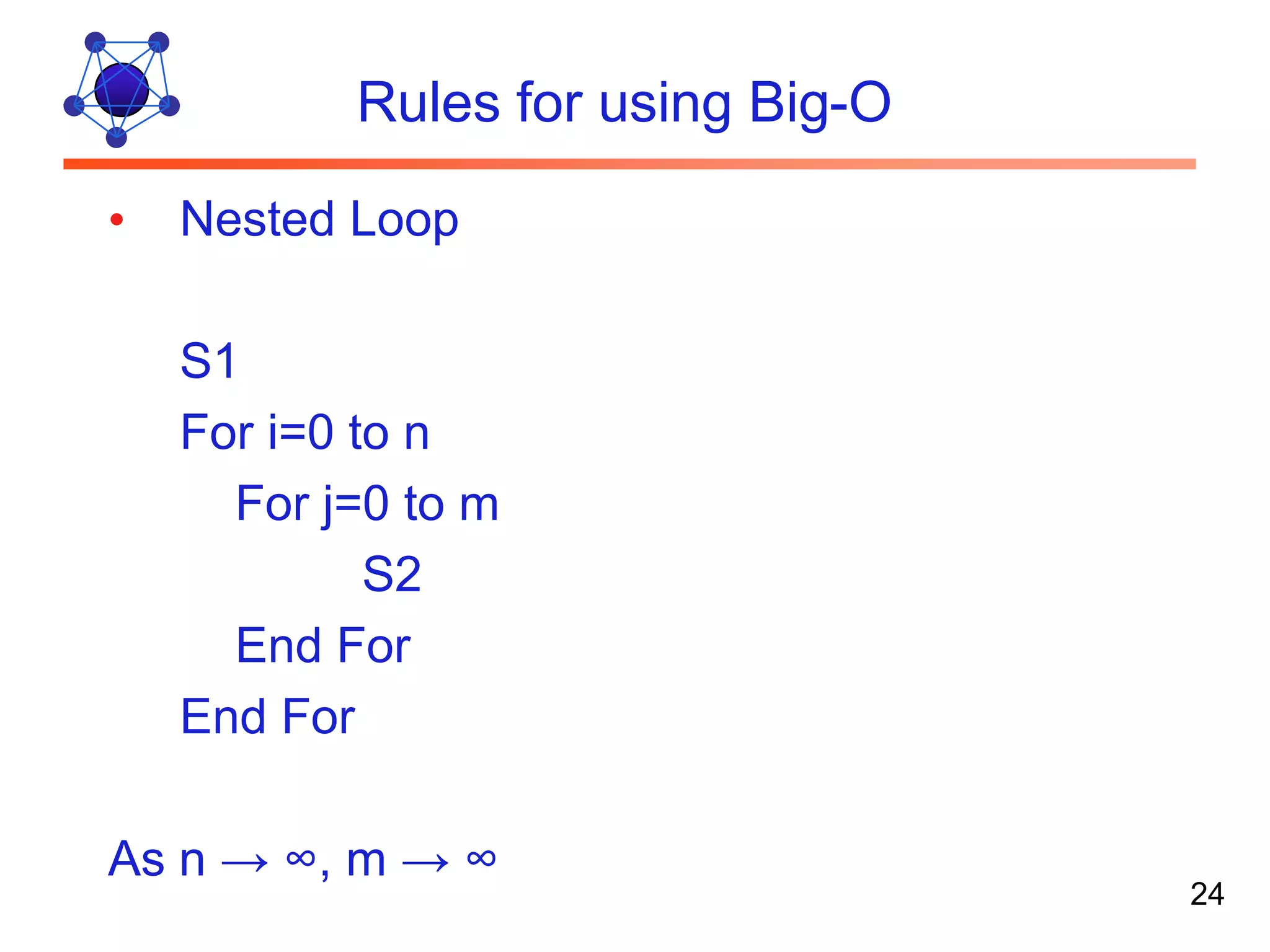
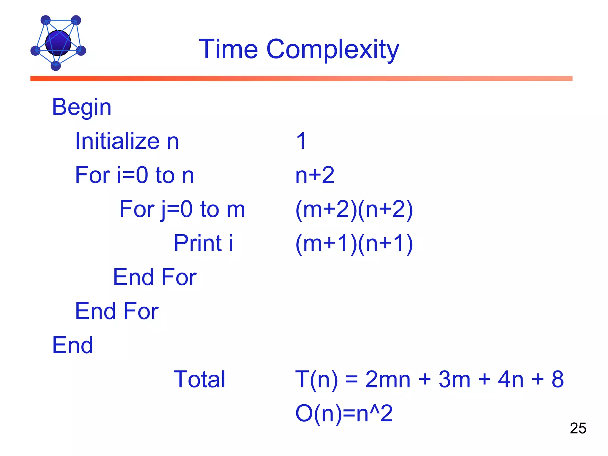
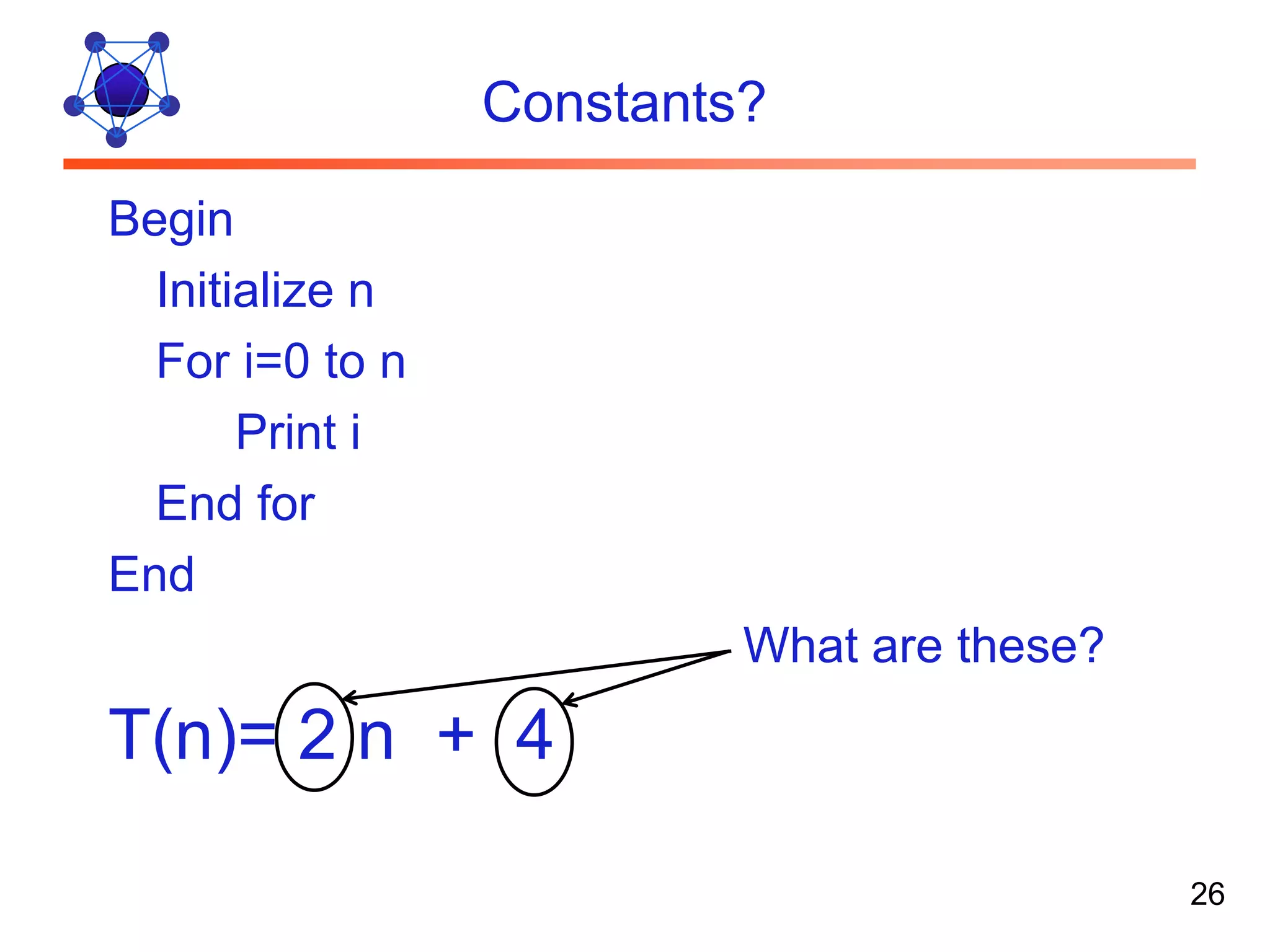
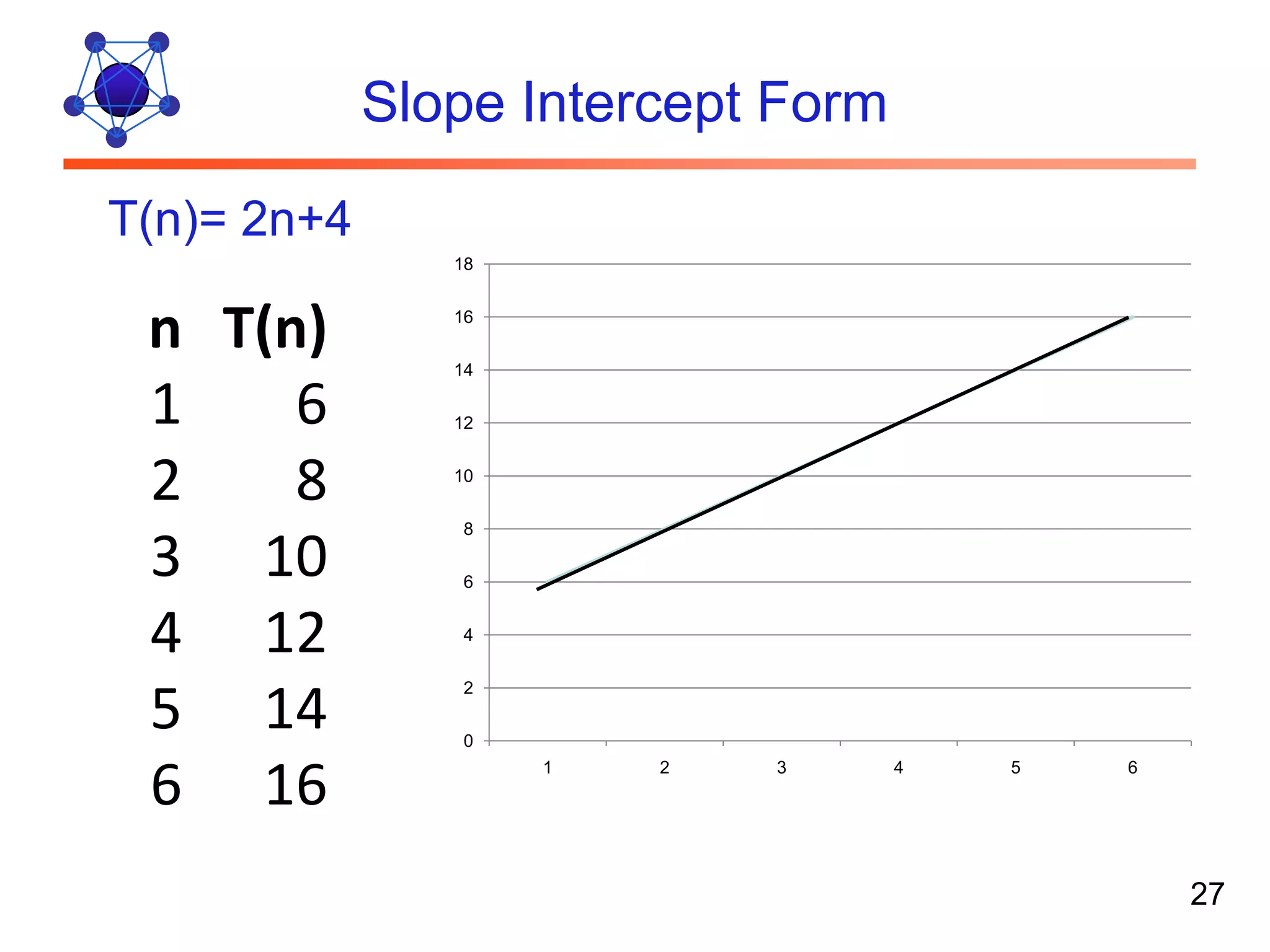
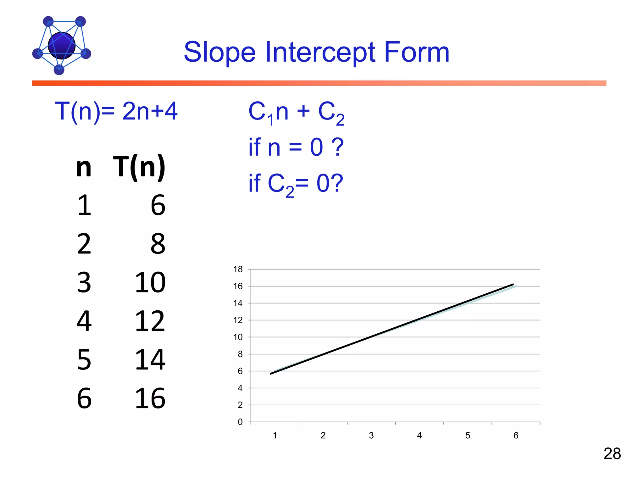
Definition Algorithm: Steps of problem solving well defined Analysis: 1. Study Performance Characteristics of Algorithms: Time and Space 2. Know the existing ways of problem solving 3. Evaluate its suitability for a particular problem 1

Properties of Algorithm Algorithm: • Precision • Determinism • Finiteness • Correctness • Generality 2

Basics of Studying Algorithms o Independent of Hardware o Op. Systems, Compilers and Languages o Independent of Data? • Badly chosen Starting Point, Initial Condition • Intelligent selection or well defined start state • Random Selection of an element • Repeat algorithm several times 3

Analysis Complexity: Goal is to classify algorithms according to their performance characteristics: Time and Space This can be done in two ways: Method 1: Absolute Value Space required: Bytes? Time required: Seconds? 4

Computational Complexity Second Method: Size of the problem represented by n Independent of machine, operating system, compiler and language used 5

Space Complexity How much Space required to execute an algorithm Unit Cost Model for memory representation Begin Initialize n variable n For i=0 to n variable i Print i Next End 6

Space Complexity Space no longer a problem Many algorithms compromise space requirements since memory is cheap Search Space grows out of bound! Swapping with secondary memory 7

Time Complexity Time required: Unit Cost Model for time Begin Initialize n For i=0 to n Print i End For End 8

Time Complexity Time required: Unit Cost Model for time Begin labels do not cost anything Initialize n 1 For i=0 to n n+2 Print i n+1 End For label End label Total T(n) = 2n+4 9

Complexity Asymptotic Complexity • Ignore machine-dependent constants --- instead of the actual running time • Look at the growth of the running time. 10

Asymptotic Complexity Example: T(n) = 2n3 T(n) = 1000n2 Which one is better? For large values of n or small values of n 11

Asymptotic Complexity We study algorithms for large values of n but that does not mean that we should forget that high complexity algorithms can execute faster if size of problem is small We focus our analysis for large values of n where n → ∞ 12

Kinds of Analysis Worst-case: (usually) • Max. time of algorithm on any input of size n. Average-case: (sometimes) • expected time over all inputs of size n. • Need assumption of statistical distribution of inputs. • Best-case: (bogus) • Cheat with a slow algorithm that works fast on some input. 13

Analysis of Algorithms Worst Case, Best Case, Average Case Example: Sorting Which one to use? For Real Time Applications Data already sorted! Is it really the best case? 14

Mathematical Notations Big-O: O (f(N) ) is bounded from above at most! Big-Omega: Ω (f(N) ) is bounded from below at least! Little-o: o (f(N) ) is bounded from above smaller than! Little-omega: ω (f(N) ) is bounded from below greater than! Theta: Θ (f(N) ) bounded, above & below equal to! 15

Big-O • O-notation is an upper-bound notation. • It makes no sense to say f(n) is at least O(n2). 16

Complexity Example: T(n) = 2n+4 Dominant Term: As n gets large enough, the dominant term has a much larger effect on the running time of an algorithm Example 2: T(n) = 2n3 + 1000n2 + 100000 17

Dominant Term Example 1: T(n) = 2n+4 Example 2: T(n) = 2n3 + 1000n2 + 100000 Remove negligible terms Example 1: n Example 2: n3 18

Dominant Term & Big-O Example 1: n Example 2: n3 We say that the algorithm runs Ex1: in the Order of n = O(n) Ex2: in the Order of n3 = O(n3) O(n) : The Time Complexity in the worst case, grows with the size of the problem 19

Rules for using Big-O • For a single statement whose execution does not depend on n: O(1) Example: i=0 • For a sequence of statement, S1,S2,…,Sk T(S1)+T(S2)+…+T(Sk) Example: i=0 O(1) + print i O(1) 20

Rules for using Big-O • Loop: For i=0 to n S1 S2 End For Dominent Term * No. of times loop executed Example: For i=0 to n j=j*8 j=j-1 End For 21

Rules for using Big-O • Conditional Loop: While i<0 S1 S2 End While No fixed rule, find a bound on the number of iterations 22

Rules for using Big-O • If condition C then S1 else S2 end if T(C) + max (T(S1) , T(S2) ) 23

Rules for using Big-O • Nested Loop S1 For i=0 to n For j=0 to m S2 End For End For As n → ∞, m → ∞ 24

Time Complexity Begin Initialize n 1 For i=0 to n n+2 For j=0 to m (m+2)(n+2) Print i (m+1)(n+1) End For End For End Total T(n) = 2mn + 3m + 4n + 8 O(n)=n^2 25

Constants? Begin Initialize n For i=0 to n Print i End for End What are these? T(n)= 2 n + 4 26

Slope Intercept Form T(n)= 2n+4 18 n T(n) 16 14 1 6 12 2 8 10 8 3 10 6 4 12 4 5 14 2 0 6 16 1 2 3 4 5 6 27

Slope Intercept Form T(n)= 2n+4 C1n + C2 if n = 0 ? n T(n) if C2= 0? 1 6 2 8 18 3 10 16 14 4 12 12 10 5 14 8 6 6 16 4 2 0 1 2 3 4 5 6 28

Order notation – some useful comparisons • O(1) < log n < n < n log n < n2 < n3 < 2n < 3n < n! < nn 31

Order notation – some useful comparisons • Behavior of Growth for Log( number, base) is the same; Log2 n = Log3 n = Log10 n 32

Practical and Un-practical algorithms • Algorithm is practical, if it’s time complexity is T(n) = O(na) (polynomial) • Algorithm is not practical otherwise T(nn) usually is exponential) 33

Example • Assume that we have a record of 1000 students. If we want to search a specific record, what is the time complexity? • If ordered? Fastest Known Sorting Algorithm (n * log n) Quick Sort / Merge Sort Fastest Known Searching Algorithm (log n) Binary Search 34

Algo complexity

More Related Content

What's hot

Viewers also liked

Similar to Algo complexity

Recently uploaded

Algo complexity