Adaptive beamforming using lms algorithm

Adaptive beamforming using lms algorithm

• 1.
  IJRET: International Journalof Research in Engineering and Technology eISSN: 2319-1163 | pISSN: 2321-7308 _______________________________________________________________________________________________ Volume: 03 Issue: 05 | May-2014, Available @ http://www.ijret.org 589 ADAPTIVE BEAMFORMING USING LMS ALGORITHM Revati Joshi1 , Ashwinikumar Dhande2 1 Student, E&Tc Department, Pune Institute of Computer Technology, Maharashtra, India 2 Professor, E&Tc Department, Pune Institute of Computer Technology, Maharashtra, India Abstract The smart antennas are widely used for wireless communication, because it has a ability to increase the coverage and capacity of a communication system. Smart antenna performs two main functions such as direction of arrival estimation (DOA) and beamforming. Using beamforming algorithm . smart antenna is able to form main beam towards desired user and null in the direction of interfering signals. This paper evaluate the performance of LMS (Least Mean Square) beamforming algorithm in the form of normalized array factor (NAF) and mean square error(MSE) by varying the number of elements in the array and the placing between the sensor elements. The simulations are carried out using MATLAB. Keywords: DOA (Direction of Arrival), LMS (Least Mean Square), AF (Array Factor). --------------------------------------------------------------------***------------------------------------------------------------------ 1. INTRODUCTION Adaptive beamforming is a technique in which an array of antennas are used to achieve maximum reception in the direction of desired user while signals of same frequency from other directions are rejected[1]. This is achieved by varying the weights of the each of antennas used in the array. A smart antenna system combines multiple antenna elements with a signal- processing capability to optimize its radiation and or reception pattern automatically in response to the signal environment[2]. Multiple antennas have ability to enhance the capacity and performance without the need of of additional power or spectrum. In adaptive beamforming the optimum weights are iteratively computed using complex algorithms based upon different criteria. The criteria for choosing the adaptive beamforming algorithm is depends on it’s performance and convergence rate. Adaptive beamforming algorithm can be classified in to two main categories such as Non blind and blind adaptive algorithms[3]. Non blind adaptive algorithms require the statistical knowledge of the transmitted signal in order to converge to a weight solution. This is achieved by using a pilot training sequence sent over the channel to receiver to help to identify the desired user. Whereas ,blind algorithms do not need any training sequence, hence the term ’blind’. They attempt to restore some characteristic of the transmitted signal in order to separate it from the other users in the surrounding environment.This paper focus on the implementation of Least Mean Square(LMS) algorithm which is a type of non blind algorithm. Fig-1: Adaptive Beamforming 2. BEAMFORMING In beamforming each user’s signal is multiplied by complex weight that adjust the magnitude and phase of the signal to and from each antenna[4]. The phases and amplitudes are adjusted to optimize the received signal. This causes the output of the arrays of antenna to form transmit or receive in a particular direction and minimizes the output in other direction Fig-2: Beamforming block diagram 3. ARRAY SENSOR SYSTEM. The system consists of ULA with M antenna elements that are linearly spaced along with equal distance. Fig 2: System model for uniform linear array of M elements
• 2.
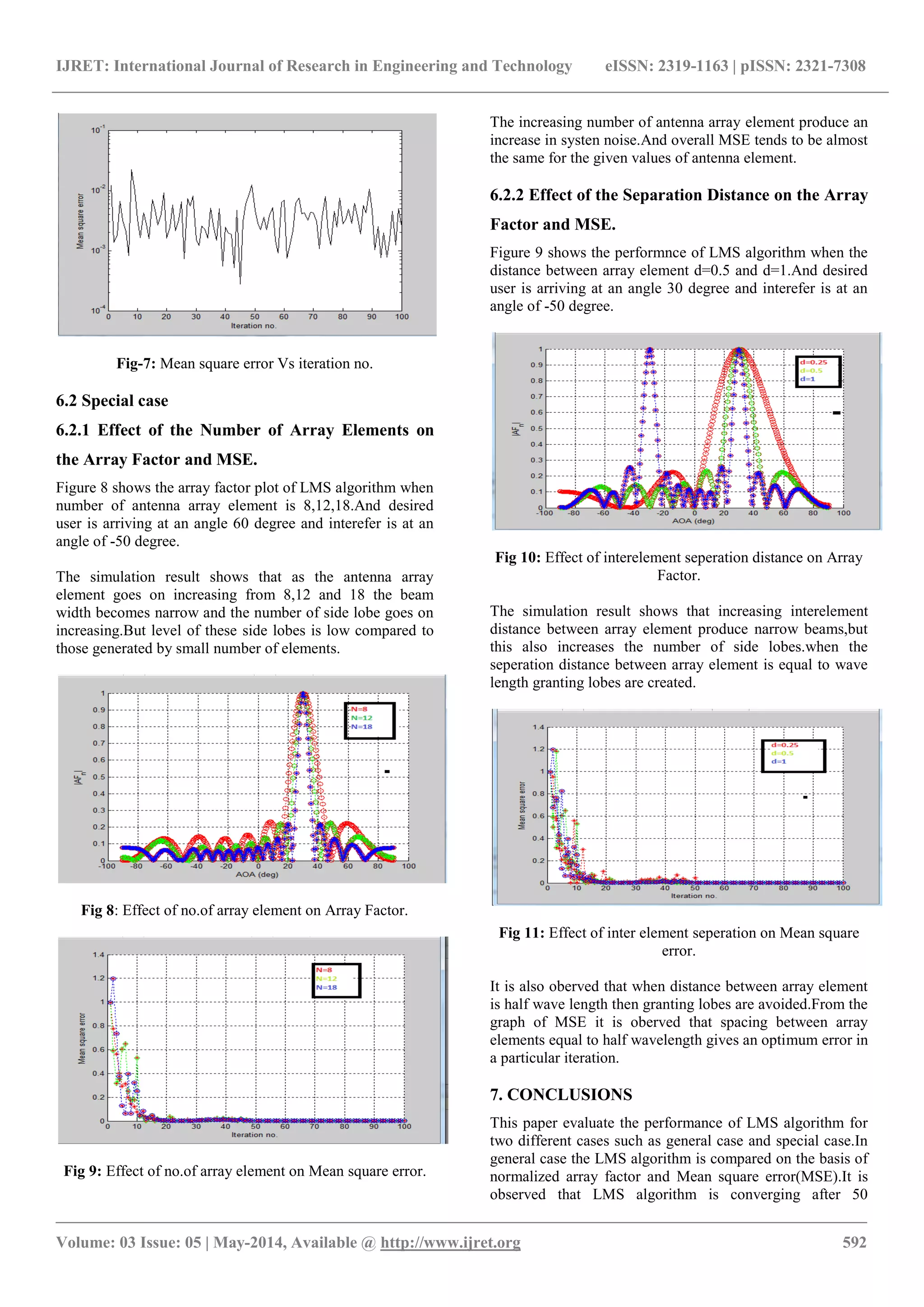
  IJRET: International Journalof Research in Engineering and Technology eISSN: 2319-1163 | pISSN: 2321-7308 _______________________________________________________________________________________________ Volume: 03 Issue: 05 | May-2014, Available @ http://www.ijret.org 590 The array factor for uniform linear array is given in eqn 1. 𝐴𝐹 ∅ = 𝐴 𝑚 𝑒 𝑗𝑚 ( 2𝜋𝑑 𝜆𝑀−1 𝑚=0 (1) The phase shift between inter element is given in eqn 2. 𝛼 = − 2𝜋𝑑 𝜆0 𝑐𝑜𝑠∅0 (2) Where, ∅0 is the desired beam direction. At wave length 𝜆0,the phase shift corresponds to a time delay that will steer the beam to∅0. 4. BASIC CONCEPT FOR LMS ALGORITHM 4.1 Weiner Optimum Solution Fig-3: LMS Adaptive Array. The LMS adaptive array is shown in figure 3. By using a feedback loop the weigths, 𝑤1,….,, 𝑤 𝑁, are updated by the time sampled error signal is given in eqn 3. e(n)=d(n)-y(n) (3) Where d(n) is training sequence or replica of the desired signal. And y(n) is the output of the adaptive array described in eqn 4 y(n)=𝑤 𝐻 x(n) (4) Where x(m) is the input signal. The adaptive algorithm adjusts the weight vector to minimize the mean square error(MSE) of the error signal,e(n) is given in eqn 5. E e(n)= E d(n)-y(n) (5) Where E is the expectation operator Substituting eqn 3 &4 in to eqn 5 and expanding the augment of the MSE term E[ 𝑒(𝑘) 2 ]=E[{d(n)-y(n)}{d(n)-𝑦(𝑛)}∗ ] (6) Solving eqn 6 obtain the value of MSE term E[ 𝑒(𝑘) 2 ]=E[ 𝑑(𝑘) 2 -𝑟𝑥𝑑 𝐻 w-𝑤 𝐻 𝑟𝑥𝑑 +𝑤 𝐻 𝑅 𝑥𝑥 w] (7) E[x(n)𝑥 𝐻 (𝑛)]=𝑅 𝑥𝑥 is the MXM covariance Matrix of the input data vector.x(n). E[x(n)𝑑∗ (𝑛)]=𝑟𝑥𝑑 is the Mx1 cross correlation vector between the input data vector ,x(n),and the training sequence,d(n). Taking the gradient operator of the mean square error with respect to the array weights and setting the result equal to zero. ∇E[ 𝑒(𝑘) 2 ]= 𝜕 𝜕𝑤 ∗E[ 𝑒(𝑘) 2 ]=0 (8) Substituting the value of eqn 7 in to eqn 8 . -2𝑟𝑥𝑑 +2𝑅 𝑥𝑥 𝑤𝑜𝑝𝑡 = 0 (9) The optimum weight eqn is obtain using eqn 10. 𝑤𝑜𝑝𝑡 =𝑅 𝑥𝑥 −1 𝑟𝑥𝑑 (10) Disadvantages using weiner optimum solution 1. If the number of elements in ULA is large ,then it is complex to invert the MXM covariance matrix ,𝑅 𝑥𝑥 [5]. 2. It requires the use of expectation operator in both 𝑅 𝑥𝑥 and𝑟𝑥𝑑 . 5. LMS ALGORITHM LMS algorithm is a type of Non-blind algorithm, because it uses the training signal or reference signal. During training period training signal is transmitted from transmitter to receiver. It uses a gradient based method of steepest decent. It follows an iterative procedure that makes successive corrections to the weight vector in the direction of the negative of the gradient vector which eventually leads to the minimum mean square error[6]. LMS algorithm is relatively simple; it does not require correlation function calculation and matrix inversions [7]. Let nw represent the Mx1 weight vector at time sample n.The weight vector can be updated at time sample n+1 which is given in eqn 11. w(n+1)=w(n)+µ[-∇(J(n))] (11) Where J(n)= E[ 𝑒(𝑛) 2 ] defines the MSE cost function. Using eqn 9,the value of the error signal at time sample n is given as in eqn 12. ∇(J(n))= -2𝑟𝑥𝑑 +2𝑅 𝑋𝑋 𝑤(𝑛) (12)
• 3.
  IJRET: International Journalof Research in Engineering and Technology eISSN: 2319-1163 | pISSN: 2321-7308 _______________________________________________________________________________________________ Volume: 03 Issue: 05 | May-2014, Available @ http://www.ijret.org 591 Substituting eqn 12 in to eqn 11 result in eqn 13 w(n+1)=w(n)+2µ[ 𝑟𝑥𝑑 − 𝑅 𝑥𝑥 𝑤(𝑛)]] (13) Where µ is step size parameter. It is a real valued positive constant generally less than one. The initial weight w(0) is assumed to be zero. The successive corrections of the weight vector eventually leads to the minimum value of the mean squared error. The step size varies from 0 to λmax, whereλ max is the largest Eigen value of the correlation matrix R[8]. Substituting the value of 𝑟𝑥𝑑 and 𝑅 𝑥𝑥 in to eqn 13 result in eqn 14. w(n+1)=w(n)+2µE[x(n)𝑒∗ (n)] (14) 6. SIMULATION RESULTS For simulation purposes the uniform linear array with M number of element and input signal is modulated by using BPSK modulation is considered. simulation of LMS algorithm is carried out using MATLAB to illustrate how various parameters such as number of antenna element, inter element spacing ,number of interferes and variation in SNR parameter affect the beam formation and convergence of the algorithm. 6.1 General case Consider that the desired user is arriving at an angle of 30 degree and an interfere user at an angle of -50 degree. The spacing between the individual element is half wavelength and the signal to noise ratio(SNR) is 30db. The array factor for 8 element antenna antenna array is computed.Figure.4.Shows rectangular array factor plot for different angle of arrival. Figure.5.Shows polar array factor plot for different angle of arrival Fig-4: Array factor plot when desired user is 30degree and the interfere is -50degree Fig-5: Polar array factor plot when desired user is 30degree and the interfere is -50degree The optimum complex weights in the case for which the algorithm converges is as follows. w1 = 1. w2 = 0.039512+0.97006i w3 = -1.0194+0.03523i w4 = -0.001461-0.98315i w5 = 0.98244-0.051033i w6 = 0.018318+1.0197i w7 = -0.97044+0.012622i w8 = -0.052976-0.99924i Fig-5: Magnitude of array weights when no.of array element is 8. Fig-6: Acquisition and tracking of desired signal and actual array output
• 4.
  IJRET: International Journalof Research in Engineering and Technology eISSN: 2319-1163 | pISSN: 2321-7308 _______________________________________________________________________________________________ Volume: 03 Issue: 05 | May-2014, Available @ http://www.ijret.org 592 Fig-7: Mean square error Vs iteration no. 6.2 Special case 6.2.1 Effect of the Number of Array Elements on the Array Factor and MSE. Figure 8 shows the array factor plot of LMS algorithm when number of antenna array element is 8,12,18.And desired user is arriving at an angle 60 degree and interefer is at an angle of -50 degree. The simulation result shows that as the antenna array element goes on increasing from 8,12 and 18 the beam width becomes narrow and the number of side lobe goes on increasing.But level of these side lobes is low compared to those generated by small number of elements. Fig 8: Effect of no.of array element on Array Factor. Fig 9: Effect of no.of array element on Mean square error. The increasing number of antenna array element produce an increase in systen noise.And overall MSE tends to be almost the same for the given values of antenna element. 6.2.2 Effect of the Separation Distance on the Array Factor and MSE. Figure 9 shows the performnce of LMS algorithm when the distance between array element d=0.5 and d=1.And desired user is arriving at an angle 30 degree and interefer is at an angle of -50 degree. Fig 10: Effect of interelement seperation distance on Array Factor. The simulation result shows that increasing interelement distance between array element produce narrow beams,but this also increases the number of side lobes.when the seperation distance between array element is equal to wave length granting lobes are created. Fig 11: Effect of inter element seperation on Mean square error. It is also oberved that when distance between array element is half wave length then granting lobes are avoided.From the graph of MSE it is oberved that spacing between array elements equal to half wavelength gives an optimum error in a particular iteration. 7. CONCLUSIONS This paper evaluate the performance of LMS algorithm for two different cases such as general case and special case.In general case the LMS algorithm is compared on the basis of normalized array factor and Mean square error(MSE).It is observed that LMS algorithm is converging after 50
• 5.
  IJRET: International Journalof Research in Engineering and Technology eISSN: 2319-1163 | pISSN: 2321-7308 _______________________________________________________________________________________________ Volume: 03 Issue: 05 | May-2014, Available @ http://www.ijret.org 593 iteration.And it has negligible error.In special case the the performance of LMS algorithm is compared on the basis of observing the effect of varying the number of antenna elements and distance between array element on the array factor and Mean square error(MSE).As number of antenna element increases the beam width of array factor becomes narrow and number of side lobe increases ,but level of side lobe is less than those generated by an array of small number of elements and overall MSE tends to be almost the same for the given values of antenna element. And spacing between array element equal to half wavelength ,then MSE gives an optimum error in a particular direction. REFERENCES [1]. D.M.M.Rahaman., Md.M.Hossair, “Least Mean Square (LMS) For Smart Antenna”, Universal Journal of Communications and Network”,pp-16-21,2013. [2]. M.Jain., V.Gupta., “Performance Analysis of MUSIC LMS Algorithm for Smart Antenna”, International Journal of Scientific Engineering and Technology,Vol.2,Issue 10,pp1004-1007,2013. [3]. U.Chalva., Dr.P.V.Humgund., “Performance Study of a Non-blind Algorithm for Smart Antenna System”, International Journal of Electronics and Communication Engineering”, Vol.5,Issue 4,pp.447-455,2012. [4]. V.Kumar., Dr.Rajouria., “Performance Analysis of LMS Adaptive Beamforming Algorithm”, International Journal of Engineering and Communication Technology,Vol.4,Issue 5,July-Sept-2013. [5]. Douglas,S.C, “Introduction to Adaptive Filters”, CRC Press LLC,PP-18,1999. [6]. K.S.Kumar and T.Gunasekaran., “Performance Analysis of Adaptive Beamforming Algorithms for Microstrip Smart Antennas”, International Journal of Computing Science and Communication Technologies, Vol.2,Issue 1,July2009. [7]. Simon Haykins, “Adaptive Filter Theory”, 3rd edition, 2001. [8]. K.K.Shetty, “A Novel Algorithm for Uplink Interference Suppression using Smart Antennas in Mobile Communications “ Master’s Thesis, Famu-Fsu College of Engineering, THE Florida state university, February 2004.