Rabid Euclidean direction search algorithm for various adaptive array geometries

Rabid Euclidean direction search algorithm for various adaptive array geometries

• 1.
  Bulletin of ElectricalEngineering and Informatics Vol. 10, No. 2, April 2021, pp. 856~869 ISSN: 2302-9285, DOI: 10.11591/eei.v10i2.1899  856 Journal homepage: http://beei.org Rabid Euclidean direction search algorithm for various adaptive array geometries Aseel Abdul-Karim Qasim, Adheed Hassan Sallomi, Ali Khalid Jassim Department of Electrical Engineering, Mustansiriyah University, Baghdad, Iraq Article Info ABSTRACT Article history: Received Nov 13, 2020 Revised Feb 6, 2021 Accepted Feb 20, 2021 One of the exciting technologies used to meet the increasing demand for wireless communication services is a smart antenna. A smart antenna is basically confirmed by an array of antennas and a digital beamformer unit through which cellular base station can direct the beam toward the desired user and set nulls toward interfering users. In this paper, different array configurations (linear, circular, and planer) with the REDS algorithm are implemented in the digital beam-forming unit. The wireless system performance is investigated to check the smart antenna potentials assuming Rayleigh fading channel environment beside the AWGN channel. Results show how the REDS algorithm offers a significant improvement through antenna radiation pattern optimization, sidelobe level, and interference reduction, and also the RDES algorithm proves fast convergence with minimum MSE and better sidelobe level reduction comparing with other algorithms. Keywords: Array factor Circular array Linear array Planar array Rapid Euclidean direction search Smart antenna This is an open access article under the CC BY-SA license. Corresponding Author: Aseel Abdul-Karim Qasim Department of Electrical Engineering Al-Mustansiriyah University Baghdad, Iraq Email: eng_aseel94@yahoo.com 1. INTRODUCTION Smart antennas (SA) were called also adaptive arrays [1, 2]. This term represents the capacity of the antenna to adjust to the condition of the communication channel in which it works. SA arrays with adaptive beam-forming capability are very efficient in suppressing interference and multi-path signals and improving signal quality by reducing the fading effects [3]. SA focuses on the notion of spatial processing, which is the key concept in adaptive antenna systems [4]. Arrays may produce the desired radiation characteristics by properly exciting each element with certain amplitudes and phases to maximize the signal from the desired users [5]. This paper analyzed various array geometries such as uniform linear (LA), uniform rectangular (PA), and circular arrays (CA). The LA has excellent direct and narrowest main beam lobe in a wanted direction, but in all azimuthal directions it does not work equally well, a major drawback of the PA is the question of presence on the opposite side of an additional large lobe of the same strength [6] the symmetry of the CA structure provides an obvious benefit since, it has no edge components, without a major change in the beamform, directional patterns synthesized with a CA can be rotated electronically in the array plane [7]. Many algorithms have been introduced to applicants on SA [8, 9], one of the most public algorithms is least mean square (LMS) A commonly employed algorithm due to its low computational complexity and ease of implementation [10]. Other less square algorithms, such as recursive least squares (RLS), conjugate gradient (CG), will converge more easily and have a lower stable mean square error (MSE) than LMS [11]. However, their high computational complexity makes them inadequate for many real-time applications [12, 13]. For adaptive filtering applications, the RDES algorithm is investigated called the Euclidean direction search
• 2.
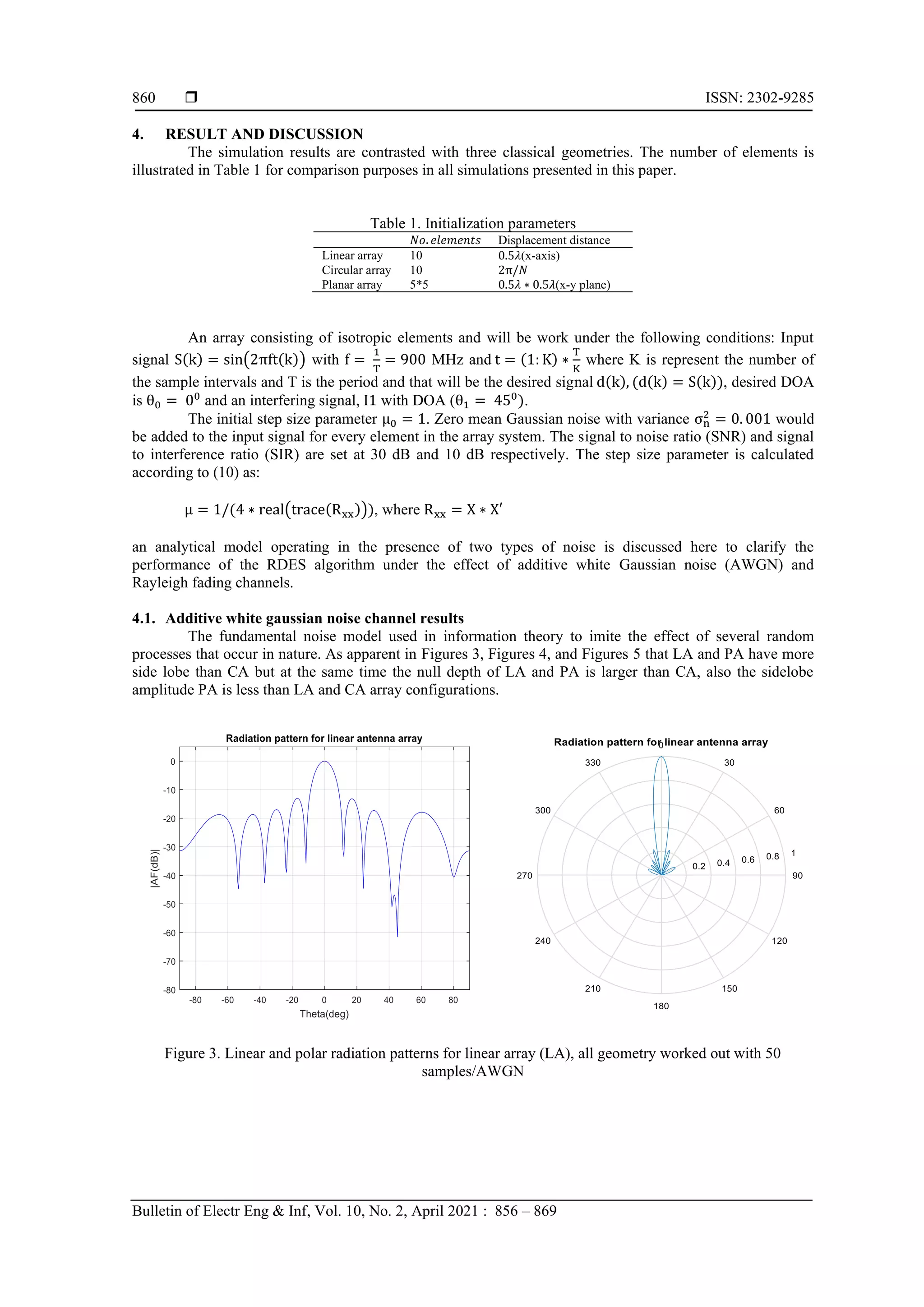
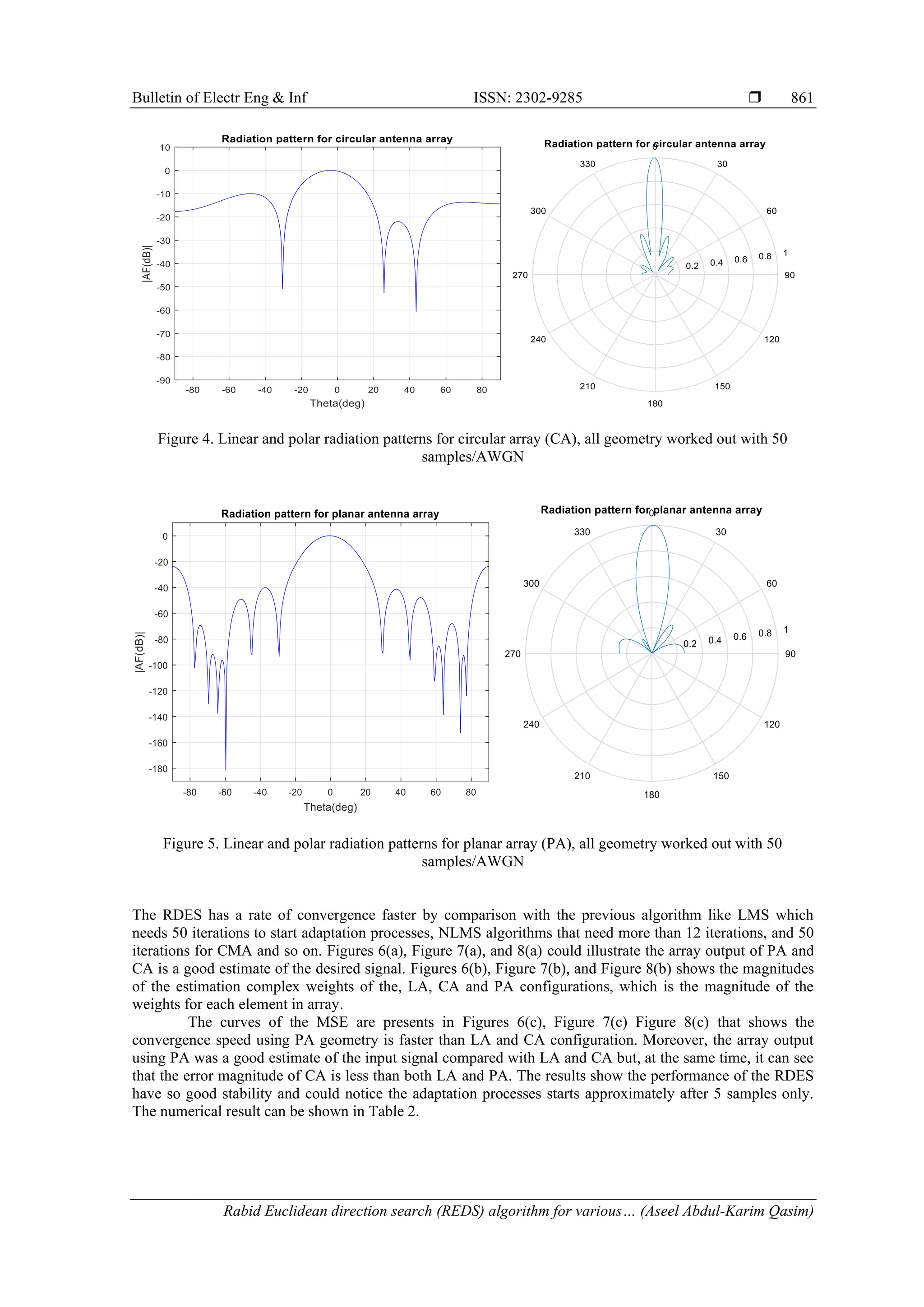
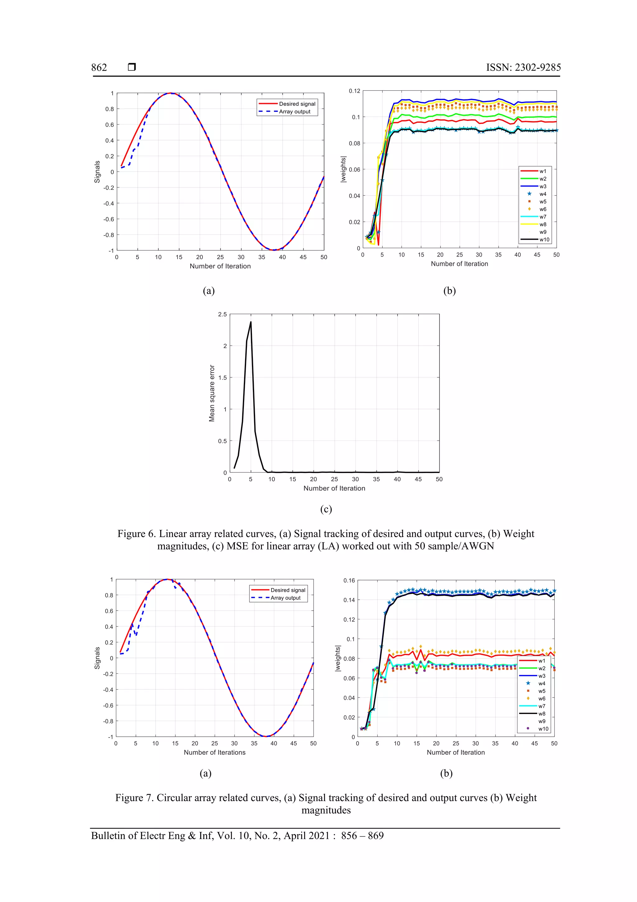
  Bulletin of ElectrEng & Inf ISSN: 2302-9285  Rabid Euclidean direction search (REDS) algorithm for various… (Aseel Abdul-Karim Qasim) 857 (EDS) since it searches cyclically for the minimum along one Euclidean direction at a time [14, 15]. These algorithms are investigated for decision feedback equalization in a mobile communication channel with additive noise and multipath. The RDES algorithm has a slower convergence rate than the Euclidean direction search (EDS) but a lot faster than the LMS [16, 17]. Also, the performance in terms of bit error rate (BER) and convergence rate is comparable to those of the RLS algorithm but at a much lower computational cost. The achievement of this work is organized by using the RDES algorithm [18, 19], with different array geometry for mobile communications. The result is analyzing by the RDES algorithm implemented by an EDS procedure to different array geometry and study the mathematical effect of array radiation pattern with applying AWGN and Rayleigh fading channels on interference suppression capability (null depth), mean square error (MSE), stability and convergence rate. 2. RADIATION PATTERN FOR ANTENNA ARRAY SYSTEM The radiation pattern in most cases defined in the far field area and is interpreted as the directional coordinate's function [20]. Antennas with a given radiation pattern can be configured to create a various radiation pattern in a system with different dimensions. For an antenna array of identical elements, the radiation pattern of the array can be defined according to the pattern multiplication theorem [21]: Array pattern = Array element pattern x Array factor In which the pattern of an array element is the pattern of the single array element, and the array factor is a feature that depends only on the array geometry and the excitation of the elements (amplitude and phase). 2.1. Linear array Figure 1(a) illustrated LA system, for simplification purposes assumption an equally spaced elements and equal amplitudes. However, each successor element has a (δ) progressive step leading current excitation compared to the past one (δ is the phase in which the current leads the current of the preceding element in each element). Assuming that the nth element leads the (n-1) element by an electrical phase shift of δ radians and can implement by shifting a phase of the antennas current for each individual element axis and the phase shift δ is equal to zero. The AF for N elements can be considered as: AF = [1 + ej(kdsin θ+δ) + ej2(kdsin θ+δ) … . ej(N−1)(kdsin θ+δ) ]T (1) and, 𝑘 = 2 ∗ 𝑝𝑖 𝜆 is the phase constant, d is element spacing, θ is arrival angle. In (2) can be expressed by, AF = ∑ 𝑊 𝑛 𝑒𝑗(𝑛−1)𝜓 𝑁 𝑛=1 (2) where, 𝜓 = 𝑘𝑑 𝑠𝑖𝑛𝜃 + δ and δ = −(𝑘𝑑 + 𝑠𝑖𝑛𝜃) which is the progressive phase, k is the wavenumber and, 𝑊𝑛 = 𝑎𝑛 ∗ 𝑒𝑗𝑏 (3) 2.2. Circular array Figure 1(b) shows CA in the x-y plane, with uniform angular distribution between elements of value ∅𝑛 = 2𝜋(𝑛−1) 𝑁 . The nth array element is positioned with the phase angle 𝜑𝑛 element at the radius (a). Every element can get a related weight 𝑤𝑛 and phase 𝛿𝑛. Also assuming far field conditions and conclude that the observation point such that the position vectors 𝑟̅and 𝑟̅𝑛are parallel. The AF can be found in a similar procedure as was calculated with the LA as [22] 𝐹 = ∑ 𝑤𝑛𝑒−𝑗(𝑘𝑎𝜌 ̂ .𝑟̂+𝛿𝑛) = ∑ 𝑤𝑛𝑒−𝑗(𝑘𝑎𝑠𝑖𝑛𝜃cos (𝜑−𝜑𝑛)+𝛿𝑛) 𝑁 𝑛=1 𝑁 𝑛=1 (4)
• 3.
   ISSN: 2302-9285 Bulletinof Electr Eng & Inf, Vol. 10, No. 2, April 2021 : 856 – 869 858 2.3. Planar array This type is used to perform 2D beamforming (in an azimuth and elevation angles) with horizontal spacing of 𝑑𝑥 and vertical spacing of 𝑑𝑦 is shown in Figure 1(c). The AF for PA can be expressed as combining the AF of two LAs [23]. Pattern multiplication can be used to calculate the pattern of the entire M×N antenna array. Utilize pattern multiplication would have: 𝐴𝐹 = 𝐴𝐹𝑥. 𝐴𝐹𝑦 = ∑ 𝑎𝑚𝑒𝑗(𝑚−1)(𝑘𝑑𝑥𝑠𝑖𝑛𝜃cos𝜑+𝛽𝑥) 𝑀 𝑚=1 ∑ 𝑏𝑛𝑒𝑗(𝑛−1)(𝑘𝑑𝑦𝑠𝑖𝑛𝜃sin𝜑+𝛽𝑦) 𝑁 𝑛=1 (5) 𝐴𝐹𝑥𝑦 = ∑ ∑ 𝑁 𝑛=1 𝑤𝑚𝑛𝑒𝑗[(𝑚−1)(𝑘𝑑𝑥𝑠𝑖𝑛𝜃cos𝜑+𝛽𝑥)+(𝑛−1)(𝑘𝑑𝑦𝑠𝑖𝑛𝜃sin𝜑+𝛽𝑦)] 𝑀 𝑚=1 (6) (a) (b) (c) Figure 1. (a) Linear array, (b) Circular array, (c) Rectangular array 3. ADAPTIVE ANTENNA ARRAY USING RDES ALGORITHM Figure 2 illustrated the block diagram of the array system. The signal S ̅(k) and interferers I1(k), I2(k), … IN(k) are received by an array of N elements with N potential weights. Each received signal at elements n includes the noise. Time is represented by kth time samples. The weighted array output can be given as: Figure 2. Block diagram for smart antenna y = w ̅H(k). x ̅(k) (7) and, x ̅(k) = a ̅0S(k) + [a ̅1 a ̅2 … . a ̅N] . [ I1(k) I2(k) ⋮ I(k) ] + n ̅(k) = x ̅S(k) + x ̅I(k) + n ̅(k) = input signal (8)
• 4.
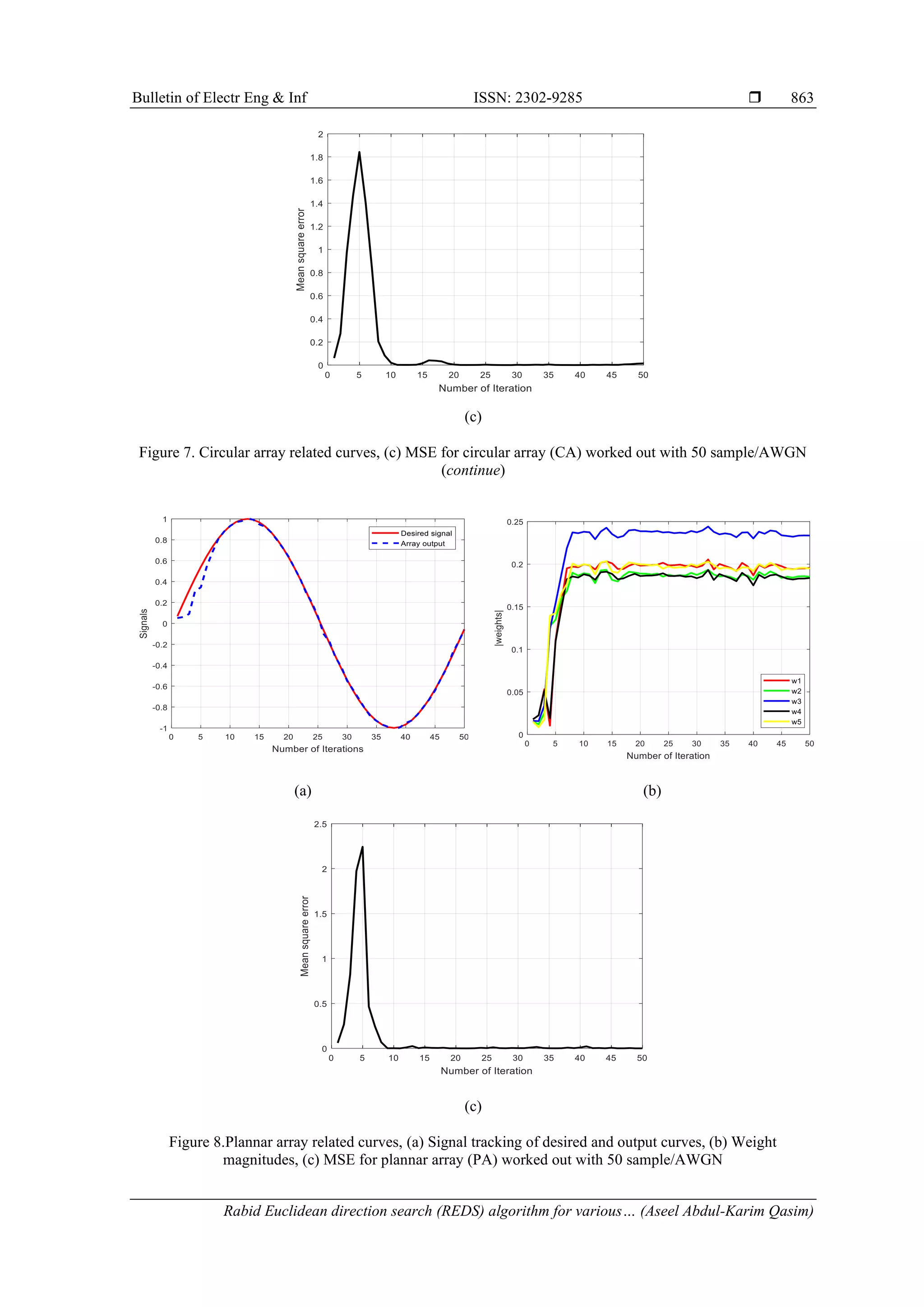
  Bulletin of ElectrEng & Inf ISSN: 2302-9285  Rabid Euclidean direction search (REDS) algorithm for various… (Aseel Abdul-Karim Qasim) 859 x ̅S(k) is the desired signal vector, x ̅I(k) is the interfering signals vector. n ̅(k) the zero-mean Gaussian noise for the channels. ai ̅Are the N element array steering vector for θ𝐼 is the arrival direction. The error signal is e(k) which defined as the difference of desired signal d(k) and output signal y(k) in the method of steepest-descent, on the other hand, a weight vector is chosen to minimize the ensemble average of the error squares [17]. The step-size parameter μ governs the convergence of algorithm because it is directly proportional to it, therefore, imperative to choose a step-size in a range that ensures convergence [1, 24, 25]. The reformulation written with RDES, the error signal, and the weight vector can give as: e(k) = d(k) − w ̅ H (k)x ̅(k) (9) w ̅(k + 1) = w ̅(k) + μ e∗(k)x ̅(k) (10) where the input and desired signals are x ̅(k) = [x1 x2 … . xM]T &d ̅ = [d(1)d(2) … . d(K)]T . The error signal e(k) can be expressed as: e(k) = d(k) − ∑ wi(k)xi(k) M i=1 (11) Considering the samples k-L, k-L+1, k-L+2 …... k, where L>M, in (11) would write as: e ̅(k) = d ̅(k) − U(k)w ̅(k) (12) where, d ̅(k) = [d(k), d(k − 1), d(k − 2) … d(k − L + 1)]T (13) U ̅(k) = [u ̅1(k), u ̅2(k) … . u ̅M(k)] (14) u ̅j(k) = [xj(k), xj(k − 1) … xj(k − L + 1)]T (15) The new approximation error at time k is given by, e ̅0(k) = d ̅(k) − U ̅(k − 1)w ̅(k − 1) (16) By update only one weight in w ̅(k − 1) the new error can be written as [26]: e ̅1(k) = d ̅(k) − [U(k)w ̅(k − 1) + U(k) w ̅j0(k) update (k) Fj0(k)] (17) j0(k) is the index of the weight to be updated in the zeroth P-iteration iteration at time k and Fj0(k) is M x 1 vector with 1 in position j and 0 in all other positions. After selecting index j0(k), the weight is given by, w ̅j0(k)(k) = w ̅j0(k)(k − 1) + w ̅j0(k) update (k) (18) where w ̅j0(k) update (k) a projection value of the error e ̅0(k) and can be givens as: w ̅j0(k) update (k) = < e ̅0(k)u ̅j0(k)(k) > ‖u ̅j0(k)(k)‖ 2 (19) when P-iteration is equal to zero the updates the array weight written with the step-size of as follows: w ̅ o(k) = w ̅(k − 1) + μRDES w ̅j0(k) update (k) Fj0(k) (20) The optimized value of μRDES can calculate by applying the same parameter (μ) used in (10).
• 5.
   ISSN: 2302-9285 Bulletinof Electr Eng & Inf, Vol. 10, No. 2, April 2021 : 856 – 869 860 4. RESULT AND DISCUSSION The simulation results are contrasted with three classical geometries. The number of elements is illustrated in Table 1 for comparison purposes in all simulations presented in this paper. Table 1. Initialization parameters 𝑁𝑜. 𝑒𝑙𝑒𝑚𝑒𝑛𝑡𝑠 Displacement distance Linear array 10 0.5𝜆(x-axis) Circular array 10 2π/𝑁 Planar array 5*5 0.5𝜆 ∗ 0.5𝜆(x-y plane) An array consisting of isotropic elements and will be work under the following conditions: Input signal S(k) = sin(2πft(k)) with f = 1 T = 900 MHz and t = (1: K) ∗ T K where K is represent the number of the sample intervals and T is the period and that will be the desired signal d(k), (d(k) = S(k)), desired DOA is θ0 = 00 and an interfering signal, I1 with DOA (θ1 = 450 ). The initial step size parameter µ0 = 1. Zero mean Gaussian noise with variance σn 2 = 0. 001 would be added to the input signal for every element in the array system. The signal to noise ratio (SNR) and signal to interference ratio (SIR) are set at 30 dB and 10 dB respectively. The step size parameter is calculated according to (10) as: μ = 1/(4 ∗ real(trace(Rxx))), where Rxx = X ∗ X′ an analytical model operating in the presence of two types of noise is discussed here to clarify the performance of the RDES algorithm under the effect of additive white Gaussian noise (AWGN) and Rayleigh fading channels. 4.1. Additive white gaussian noise channel results The fundamental noise model used in information theory to imite the effect of several random processes that occur in nature. As apparent in Figures 3, Figures 4, and Figures 5 that LA and PA have more side lobe than CA but at the same time the null depth of LA and PA is larger than CA, also the sidelobe amplitude PA is less than LA and CA array configurations. Figure 3. Linear and polar radiation patterns for linear array (LA), all geometry worked out with 50 samples/AWGN
• 6.
  Bulletin of ElectrEng & Inf ISSN: 2302-9285  Rabid Euclidean direction search (REDS) algorithm for various… (Aseel Abdul-Karim Qasim) 861 Figure 4. Linear and polar radiation patterns for circular array (CA), all geometry worked out with 50 samples/AWGN Figure 5. Linear and polar radiation patterns for planar array (PA), all geometry worked out with 50 samples/AWGN The RDES has a rate of convergence faster by comparison with the previous algorithm like LMS which needs 50 iterations to start adaptation processes, NLMS algorithms that need more than 12 iterations, and 50 iterations for CMA and so on. Figures 6(a), Figure 7(a), and 8(a) could illustrate the array output of PA and CA is a good estimate of the desired signal. Figures 6(b), Figure 7(b), and Figure 8(b) shows the magnitudes of the estimation complex weights of the, LA, CA and PA configurations, which is the magnitude of the weights for each element in array. The curves of the MSE are presents in Figures 6(c), Figure 7(c) Figure 8(c) that shows the convergence speed using PA geometry is faster than LA and CA configuration. Moreover, the array output using PA was a good estimate of the input signal compared with LA and CA but, at the same time, it can see that the error magnitude of CA is less than both LA and PA. The results show the performance of the RDES have so good stability and could notice the adaptation processes starts approximately after 5 samples only. The numerical result can be shown in Table 2.
• 7.
   ISSN: 2302-9285 Bulletinof Electr Eng & Inf, Vol. 10, No. 2, April 2021 : 856 – 869 862 (a) (b) (c) Figure 6. Linear array related curves, (a) Signal tracking of desired and output curves, (b) Weight magnitudes, (c) MSE for linear array (LA) worked out with 50 sample/AWGN (a) (b) Figure 7. Circular array related curves, (a) Signal tracking of desired and output curves (b) Weight magnitudes
• 8.
  Bulletin of ElectrEng & Inf ISSN: 2302-9285  Rabid Euclidean direction search (REDS) algorithm for various… (Aseel Abdul-Karim Qasim) 863 (c) Figure 7. Circular array related curves, (c) MSE for circular array (CA) worked out with 50 sample/AWGN (continue) (a) (b) (c) Figure 8.Plannar array related curves, (a) Signal tracking of desired and output curves, (b) Weight magnitudes, (c) MSE for plannar array (PA) worked out with 50 sample/AWGN
• 9.
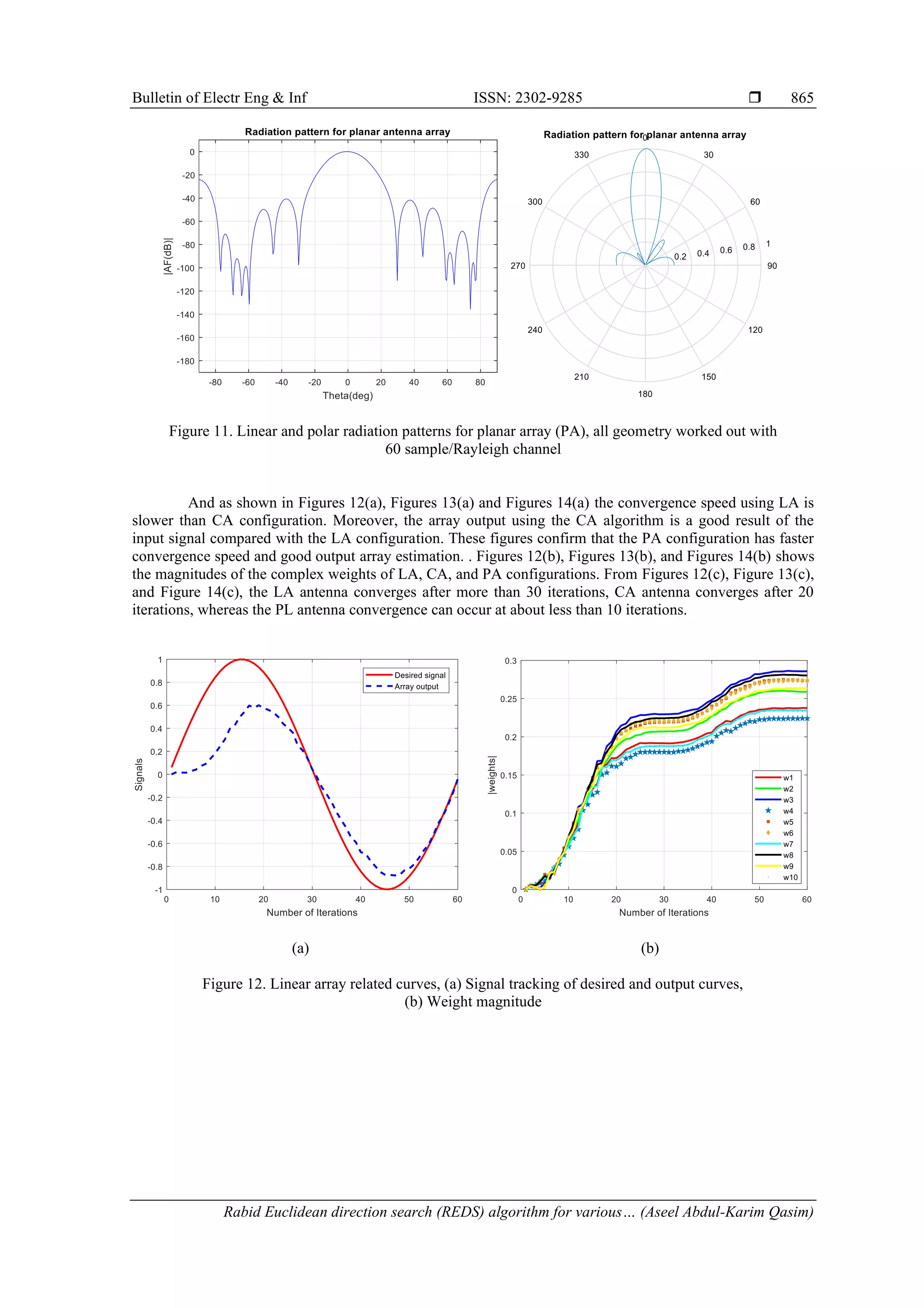
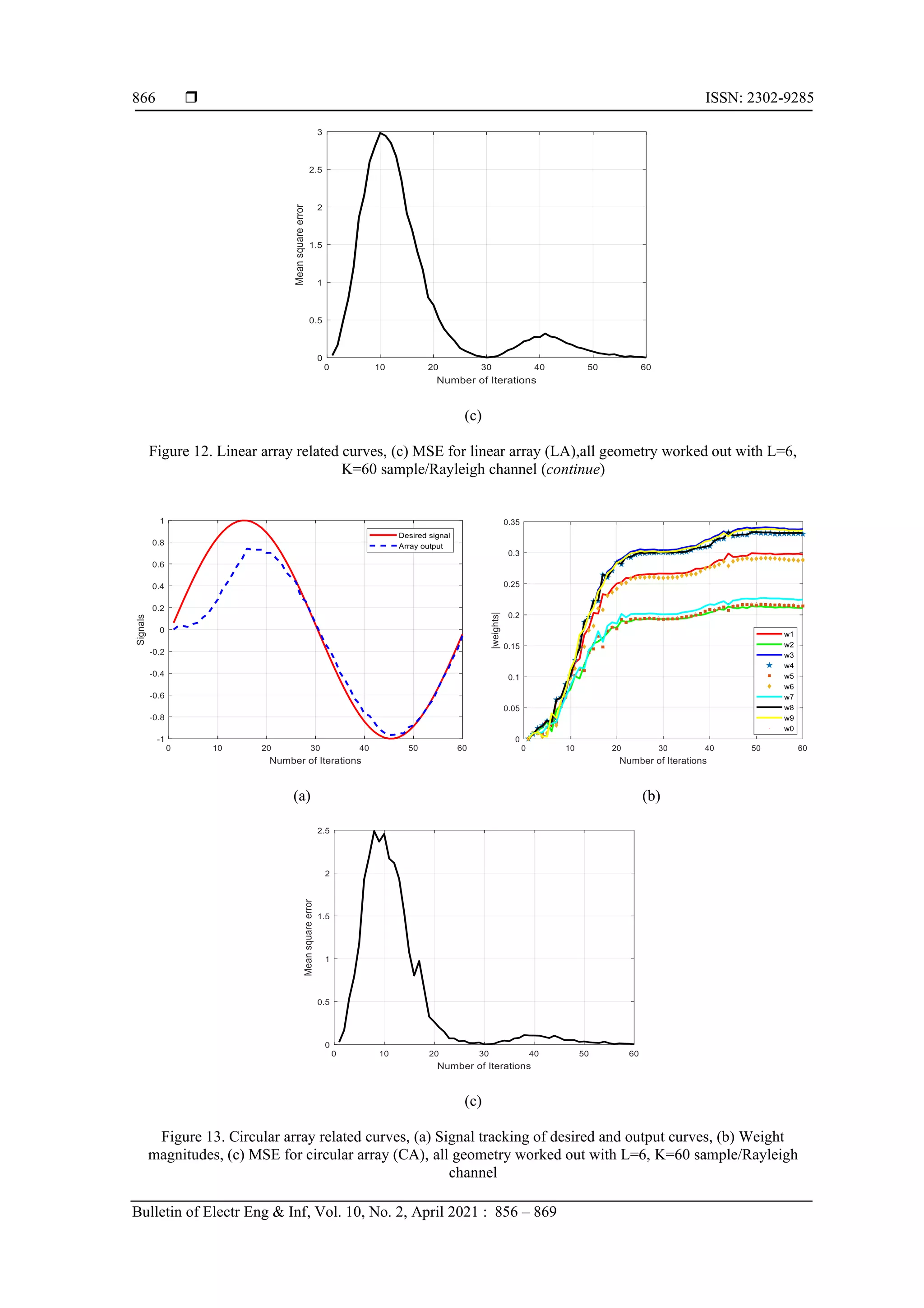
   ISSN: 2302-9285 Bulletinof Electr Eng & Inf, Vol. 10, No. 2, April 2021 : 856 – 869 864 Table 2. Additive white Gaussian noise results Depth null (dB) SLL (dB) Weight stability Maximum mean square error LA -61 -13 8 iterations 1.4089e-04 CA -60 -10 5 iterations 0.0055 PA -96 -23.6 7 iterations 1.2625e-04 4.2. Rayleigh fading channel results Rayleigh fading is the statistical model that effect on the radio signal of a propagation environment, is most applicable when several objects in an environment scatter the radio signal and that lead to no dominant propagation along a line of sight between the transmitter and receiver, such as that used by wireless devices [27]. The magnitude of a signal that has passed through such a transmission medium (a communication channel) will vary randomly is assumed. In the performance evaluation the following conditions are considered: The signals arriving at each antenna element, for the desired and interfering signal, subject to independent Rayleigh fading. Both the wanted signal and Interfering signal have the same amplitude as are emanating from 0° and 45°. Each simulation involves a run (data rate) of 500 Kbits. Doppler frequency fd of 117 Hz, corresponding to the mobility of 140 km/h at 900 MHz will be used in this simulation to present a worst case process. All antenna geometry is implemented when the number of samples is set at K=60. Figures 9, Figure 10, and Figure 11 show that the performance of the RDES which works better when compared with planar array than the LA&CA array. Figure 9. Linear and polar radiation patterns for linear array (LA), all geometry worked out with 60 sample/Rayleigh channel Figure 10. Linear and polar radiation patterns for circular array (CA), all geometry worked out with 60 sample/Rayleigh channel
• 10.
  Bulletin of ElectrEng & Inf ISSN: 2302-9285  Rabid Euclidean direction search (REDS) algorithm for various… (Aseel Abdul-Karim Qasim) 865 Figure 11. Linear and polar radiation patterns for planar array (PA), all geometry worked out with 60 sample/Rayleigh channel And as shown in Figures 12(a), Figures 13(a) and Figures 14(a) the convergence speed using LA is slower than CA configuration. Moreover, the array output using the CA algorithm is a good result of the input signal compared with the LA configuration. These figures confirm that the PA configuration has faster convergence speed and good output array estimation. . Figures 12(b), Figures 13(b), and Figures 14(b) shows the magnitudes of the complex weights of LA, CA, and PA configurations. From Figures 12(c), Figure 13(c), and Figure 14(c), the LA antenna converges after more than 30 iterations, CA antenna converges after 20 iterations, whereas the PL antenna convergence can occur at about less than 10 iterations. (a) (b) Figure 12. Linear array related curves, (a) Signal tracking of desired and output curves, (b) Weight magnitude
• 11.
   ISSN: 2302-9285 Bulletinof Electr Eng & Inf, Vol. 10, No. 2, April 2021 : 856 – 869 866 (c) Figure 12. Linear array related curves, (c) MSE for linear array (LA),all geometry worked out with L=6, K=60 sample/Rayleigh channel (continue) (a) (b) (c) Figure 13. Circular array related curves, (a) Signal tracking of desired and output curves, (b) Weight magnitudes, (c) MSE for circular array (CA), all geometry worked out with L=6, K=60 sample/Rayleigh channel
• 12.
  Bulletin of ElectrEng & Inf ISSN: 2302-9285  Rabid Euclidean direction search (REDS) algorithm for various… (Aseel Abdul-Karim Qasim) 867 (a) (b) (c) Figure 14. Plannar array related curves, (a) Signal tracking of desired and output curves, (b) Weight magnitudes, (c) MSE for plannar array (PA), all geometry worked out with L=6, K=60 sample/Rayleigh channel The results could present that the performance of the PA is better and faster than the other shapes. The numerical results with Rayleigh channel are shown in Table 3. Table 3. Rayleigh fading results Depth null(dB) SLL(dB) Weight stability Maximum mean square error LA -62 -13 40 2.4865e-04 CA -48 -6 20 0.0010 PA -90 -24 10 5.7605e-04 Figure 9, Figure 10 and Figure 11 illustrates that the PA generates the deeper null which about -90 dB towards the interferer, the LA and CA configurations provide the deep null of about -62 dB and -48 dB at K=60. It is apparent from this array pattern in Figure 9, Figure 10, and Figure 11 the CA array provides the lowest array side lobes number while PA provides the lowest array SLL compared with the other configurations. Multipath and their effects on antenna array pattern with using RDES algorithm also have been introduced, Figure 15 illustrate linear and polar plot for antenna array pattern curve under multipath signals.
• 13.
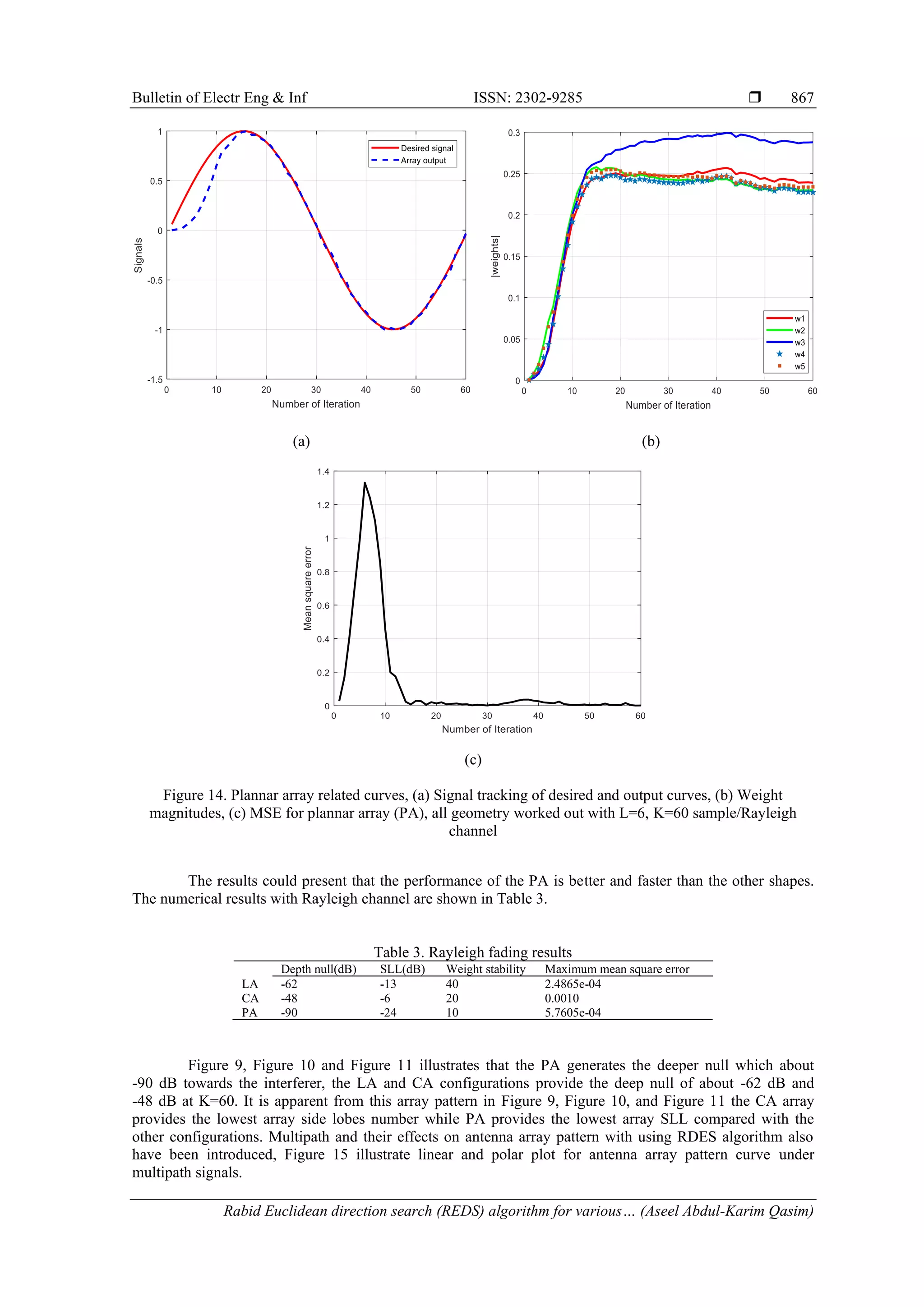
   ISSN: 2302-9285 Bulletinof Electr Eng & Inf, Vol. 10, No. 2, April 2021 : 856 – 869 868 Figure 15. Linear & polar plots, for radiation patterns with 8 elements linear array where a-desire (S)=0/Interference (I)=45, -20, b-S=0, 35/I=60, -30, c-S=0, 30/I=50, -30, -70, d-S=0, -20, 30/I=50, -45, -70, worked out with 50 sample/AWGN As illustrated in Table 4, the effectiveness of the RDES algorithm appears to guidance or steer the mean pattern beam in the direction of users and steering the depth extinct to interference directions. Table 4. Analyze multipath effect Desired DOA(S) Interference DOA(I) Depth null (dB) a 0° 45° & − 20° -48.5&-59.2 b 0° &35° 60° & − 30° -61&-41.7 c 0° &30° 50° & − 30° & − 70° -38.1&-42.3&-62.7 d 0° &30° & − 20° 50° & − 45° & − 70° -36.7&-51.2&-55.1 5. CONCLUSION The renewal in this paper is the use of the RDES algorithm in different antenna array geometries, also consideration the RDES algorithm's ability to operate under the effect of AWGN channel and Rayleigh fading environment. The result appears robust and remains stable when working in the case of Rayleigh fading and even when additive white Gaussian noise (AWGN) corrupts their reference signals. Via simulation of AWGN channel smart antennas the LA, PA, and CA begin to converge with iteration number of fewer than 10 samples. These configurations generate a deeper null towards the angles of interfering signals which is about (-61 dB for LA), (-60 dB for CA), and (-96 dB for PA). In the case of Rayleigh fading channel, the LA, CA, and PA configuration approximately converge after 20 iterations samples. The deeper null generated is (-62 dB for LA), (-48 dB for CA), and (-90 dB for PA) .The simulation results confirm that the performance of the RDES with PA has better main lobe with lower beam width but more side lobe inside of the appearance of great lobe effects, whereas CA is better in term of the number of side lobe than both LA and also PA antenna systems with fewer elements beside it's flexible angle range. ACKNOWLEDGEMENTS This work is supported by the Electrical Department, Faculty of Engineering, Mustansiriyah University. REFERENCES [1] C. Yan, “Smart antenna for wireless communication,” Telecommunication Science, vol. 5, pp. 5-10, 2002. [2] F. B. Gross, “Smart antenna for wireless communication”, Scientific Research an Academic Publisher, McGraw- Hill, Inc., USA, 2005. [3] A. A. Qasim and A. H. Sallomi, “performance improvement for smart antenna system least square beamforming algorithms,” Journal of Engineering and Sustainable Development, vol. 24, no. Special Issue, pp. 155-165, 2020.
• 14.
  Bulletin of ElectrEng & Inf ISSN: 2302-9285  Rabid Euclidean direction search (REDS) algorithm for various… (Aseel Abdul-Karim Qasim) 869 [4] M. Mouhamadou, P. Vaudon, and M. Rammal, “Smart antenna array patterns synthesis: Null steering and multi- user beamforming by phase control,” Progress in Electromagnetics Research, vol. 60, pp. 95-106, 2006. [5] A. A. K. Qasim and A. H. Sallomi, “Optimisation of adaptive antenna array performance using particle swarm algorithm,” 2019 1st Int. Sci. Conf. Comput. Appl. Sci. CAS, IEEE, pp. 137-142, 2019. [6] A. Vesa, F. Alexa, and H. Baltă, “Comparisons between 2D and 3D uniform array antennas,” 2015 Federated Conference on Computer Science and Information Systems (FedCSIS), Lodz, pp. 1285-1290, 2015. Doi: 10.15439/2015F266 [7] P. Ioannides and C. A. Balanis, “Uniform circular arrays for smart antennas,” in IEEE Antennas and Propagation Magazine, vol. 47, no. 4, pp. 192-206, Aug. 2005. [8] T. M. Jamel and B. M. Mansoor, “Application of fast Euclidean direction search (FEDS) method for smart antennas in mobile communications systems,” IET Digital Library, pp. 1-6, 2013. [9] V. Dakulagi and M. Bakhar, “Advances in smart antenna systems for wireless communication,” Wireless Personal Communications, Springer US, vol. 110, no. 2, pp. 931-957, 2010. Doi: 10.1007/s11277-019-06764-6 [10] D. N. Patel, B. J. Makwana, and P. B. Parmar, “Comparative analysis of adaptive beamforming algorithm LMS, SMI and RLS for ULA smart antenna,” 2016 International Conference on Communication and Signal Processing (ICCSP), Melmaruvathur, pp. 1029-1033, 2016. Doi: 10.1109/ICCSP.2016.7754305 [11] P. Chuku, T. Olwal, and K. Djouani, “Adaptive array beamforming using an enhanced RLS algorithm,” International Journal on AdHoc Networking Systems, vol. 8, no. 1, pp. 1-13, 2018. Doi: 10.5121/ijans.2018.8101 [12] B. Xie, “Partial update adaptive filtering,” VT Virginia Tech, Virginia Polytechnic Institute and State University, Virginia, Dec. 2011. [13] K. Dogancay and O. Tanrikulu, “Adaptive filtering algorithms with selective partial updates,” in IEEE Transactions on Circuits and Systems II: Analog and Digital Signal Processing, vol. 48, no. 8, pp. 762-769, Aug. 2001. [14] Guo-Fang Xu and T. Bose, “Analysis of the Euclidean direction set adaptive algorithm,” Proceedings of the 1998 IEEE International Conference on Acoustics, Speech and Signal Processing, ICASSP '98 (Cat. No.98CH36181), Seattle, WA, USA, vol. 3, pp. 1689-1692, 1998. [15] Ali Khalid Jassim and Raad H. Thaher, “Calculate the optimum slot area of elliptical microstrip antenna for mobile application,” Indonesian Journal of Electrical Engineering and Computer Science, vol. 16, no. 3, pp. 1364-1370, Dec. 2019. [16] A. Ropponen, M. Linnavuo, and R. Sepponen, “LF indoor location and identification system,” International Journal On Smart Sensing And Intelligent Systems, vol. 2, no. 1, pp. 94-117, 2009 [17] C. A. Balanis, “Modern antenna handbook,” John Wiley & Sons, 2011. [18] T. Mathurasai, T. Bose, and D. M. Etter, “Decision feedback equalization using an Euclidean direction based adaptive algorithm,” Conference Record of the Thirty-Third Asilomar Conference on Signals, Systems, and Computers, (Cat. No.CH37020), Pacific Grove, CA, USA, vol. 1, pp. 519-523, 1999. [19] Cheng Zhao and S. S. Abeysekera, “Investigation of Euclidean direction search based Laguerre adaptive filter for system identification,” Proceedings. 2005 International Conference on Communications, Circuits and Systems, Hong Kong, China, pp. 691-695, 2005. [20] C. A. Balanis, “Antenna theory: analysis and design,” John wiley & sons, 2016 [21] R. C. Johnson and H. Jasik, “Antenna engineering handbook,” McGraw-Hill B. Company, New York, p. 1356, 1984. [22] S. F. Shaukat, Mukhtar Ul. Hassan, and R. Farooq, “Sequential studies of beamforming algorithms for smart antenna systems,” World Applied Sciences Journal, vol. 6, no. 6, pp. 754-758, 2009. [23] S. A. Hosseini, S. A. Hadei, M. B. Menhaj, and P. Azmi, “Fast Euclidean direction search algorithm in adaptive noise cancellation and system identification,” Internatiuonal Journal of Innovative Computing, Information and Control, vol. 9, no. 1, pp. 191-206, 2013. [24] Ali Khalid Jassim and Raad H. Thaher, “Enhancement gain of broadband elliptical microstrip patch array antenna with mutual coupling for wireless communication, ” Indonesian Journal of Electrical Engineering and Computer Science, vol. 13, no. 1, pp. 217-225, 2019. [25] S. Hossain, M. T. Islam, and S. Serikawa, “Adaptive beamforming algorithms for smart antenna systems,” 2008 International Conference on Control, Automation and Systems, Seoul, pp. 412-416, 2008. [26] S. Liew, “Adaptive equalisers and smart antenna systems,” Bachelor of Engineering Thesis, The University of Queensland, Australia, pp. 1-82, Oct. 2002. [27] M. Mahboob, F. M. Sajidul Alam, and M. Sittul, “Comparison of different models for the analysis of Rayleigh fading channels,” B.Sc. Thesis, BRAC University, Dec. 2007