Downloaded 340 times

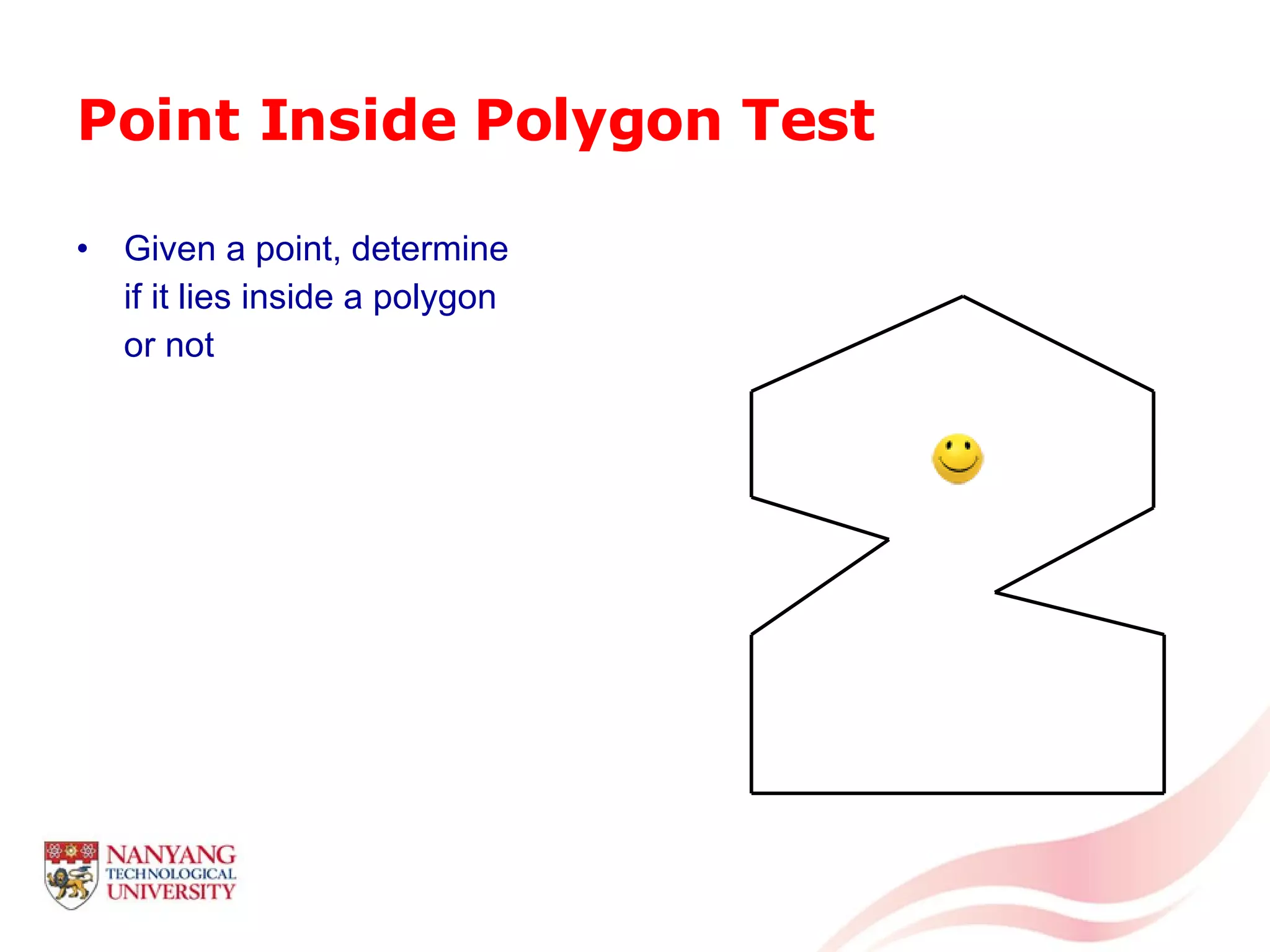
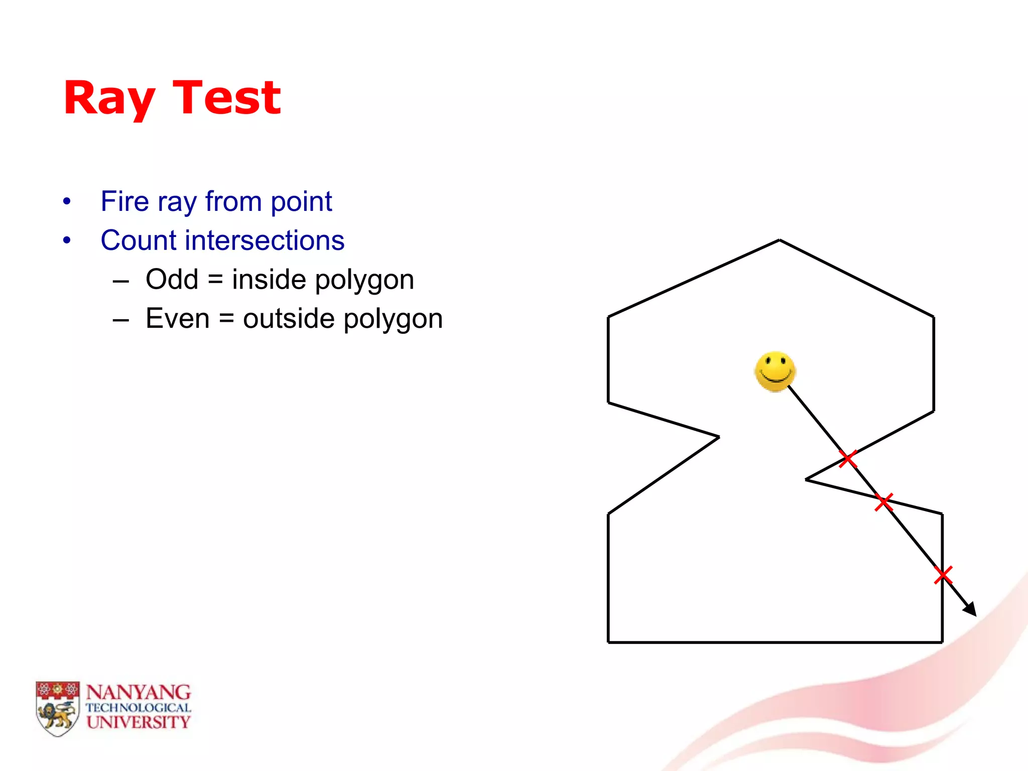
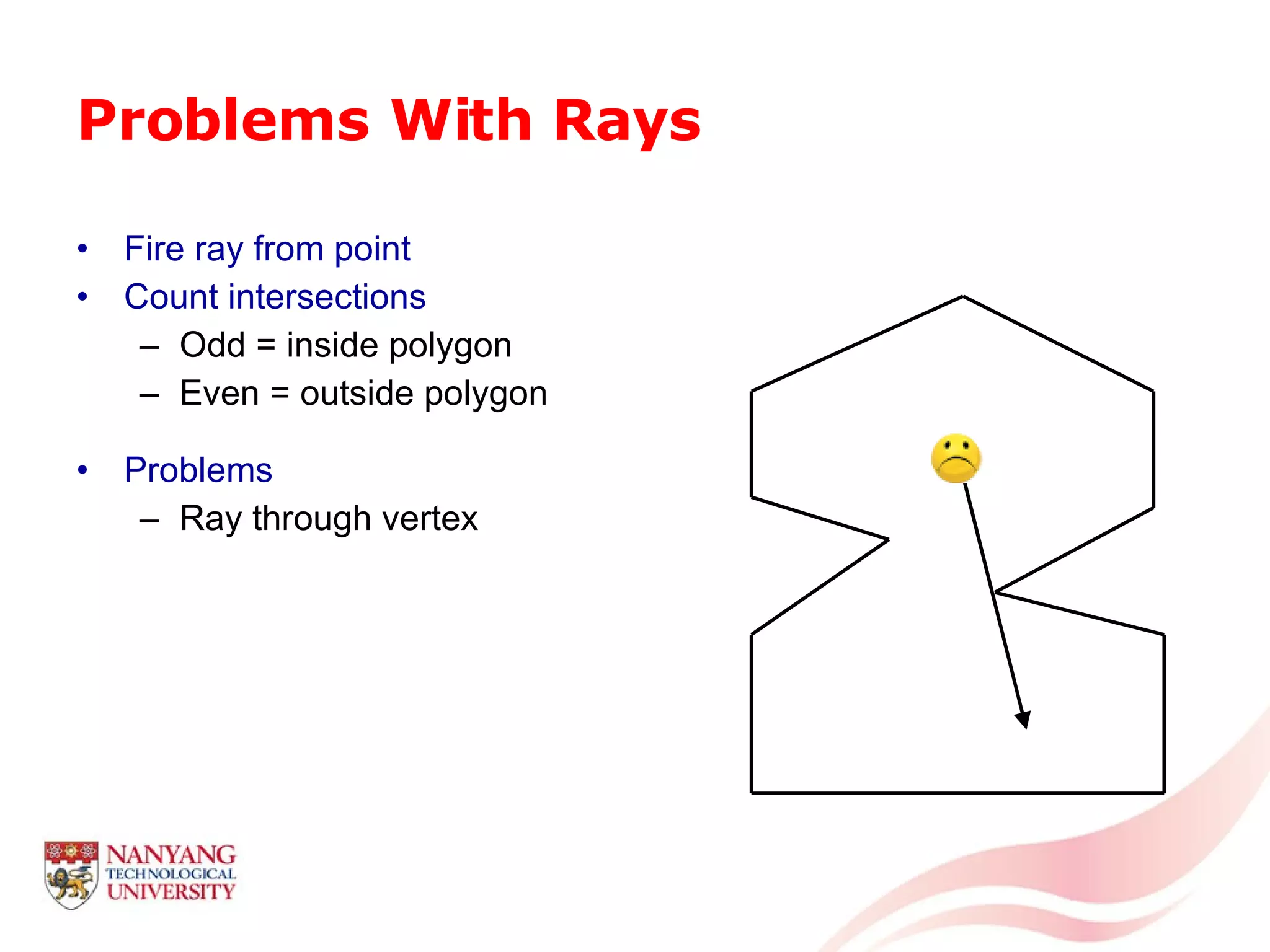
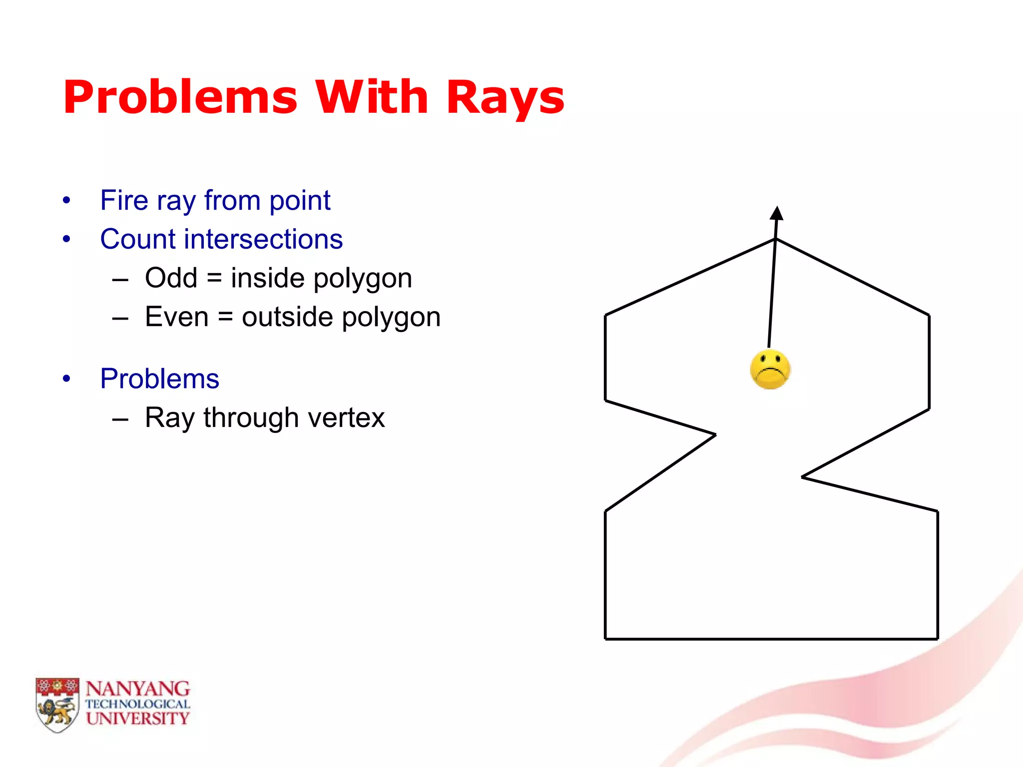
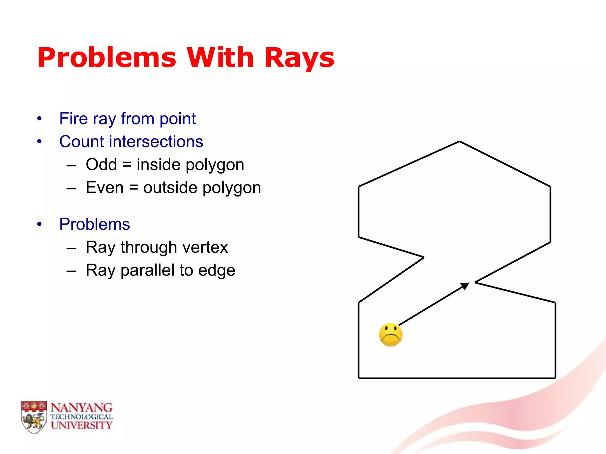

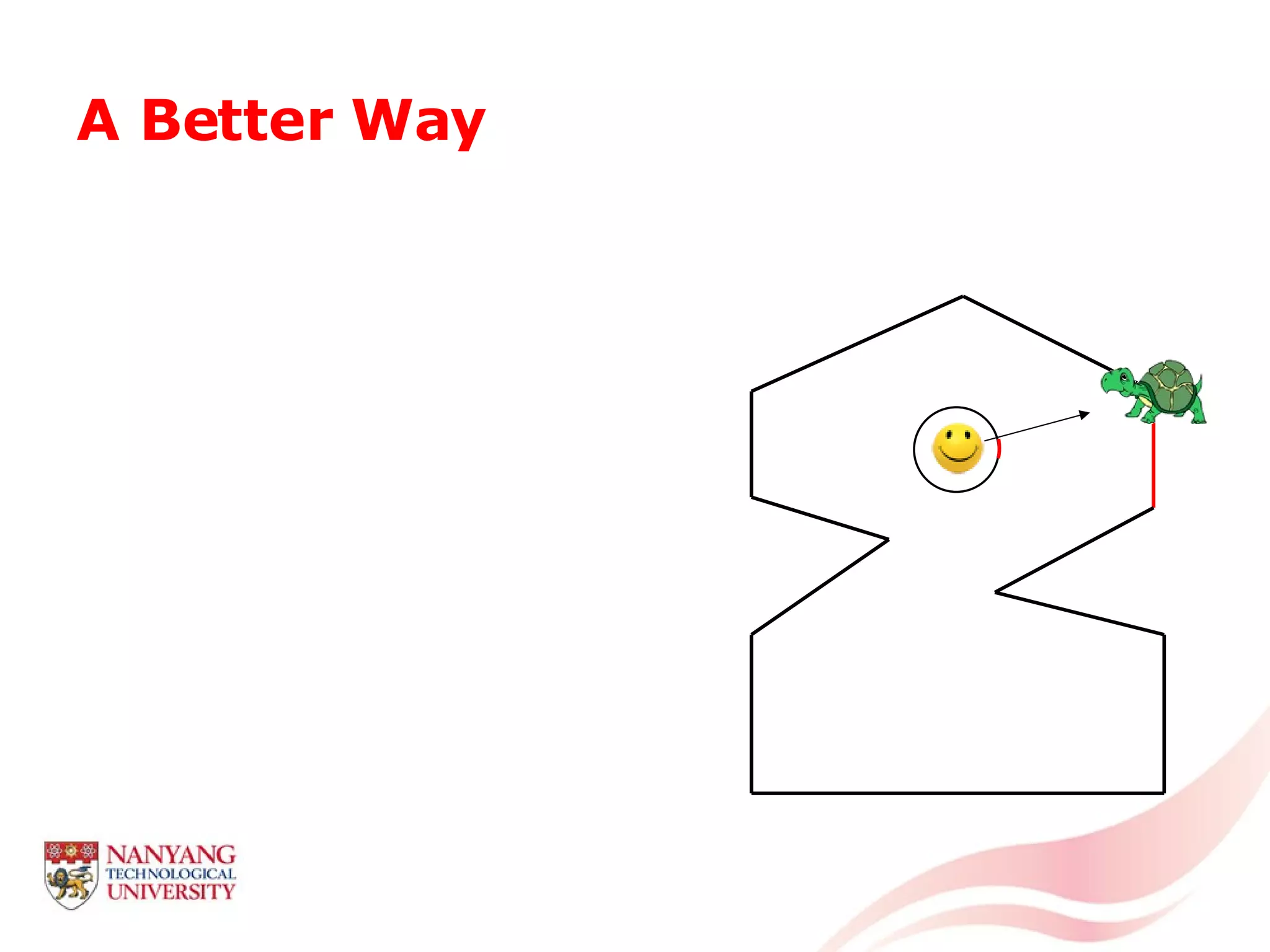


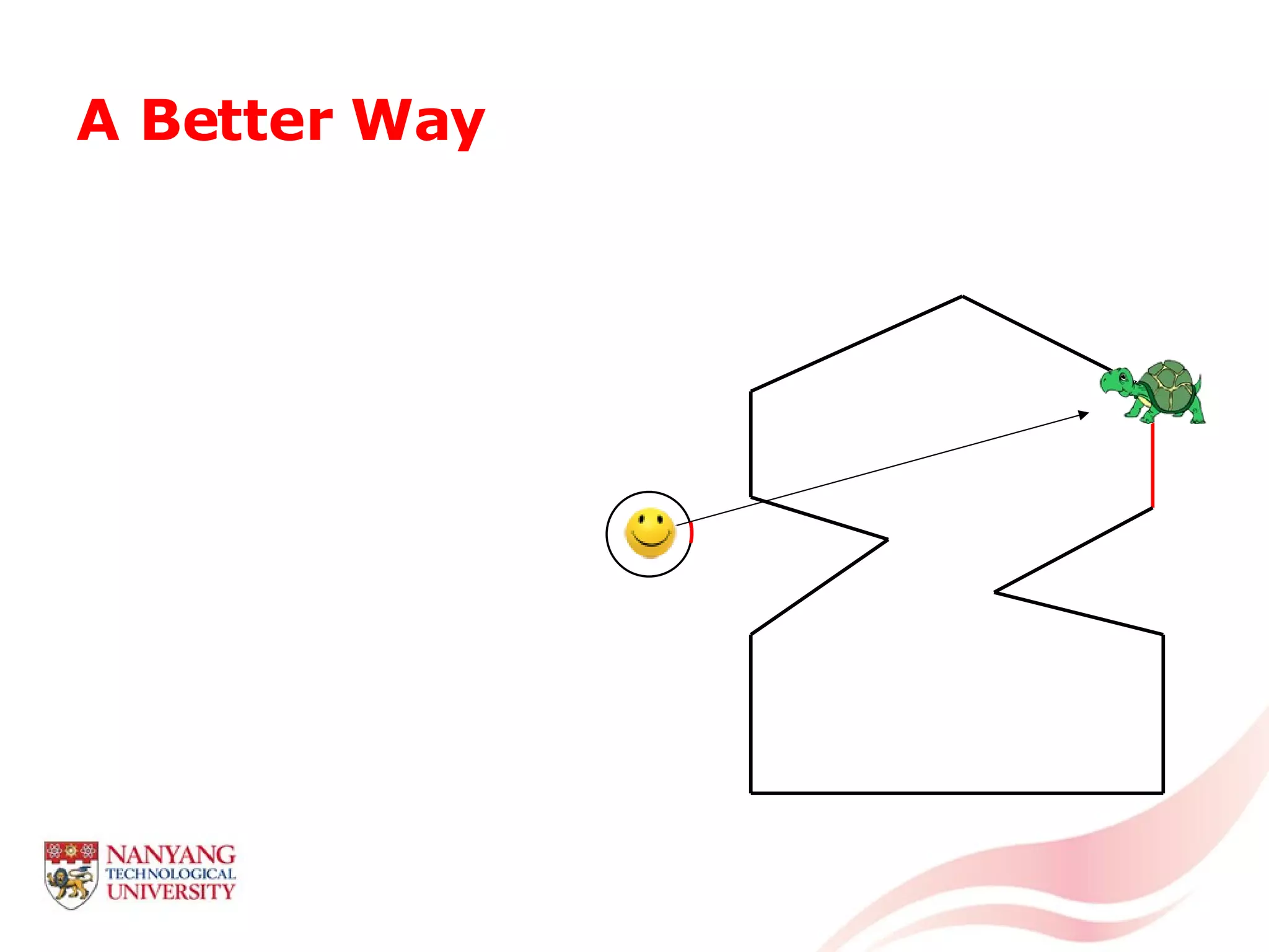


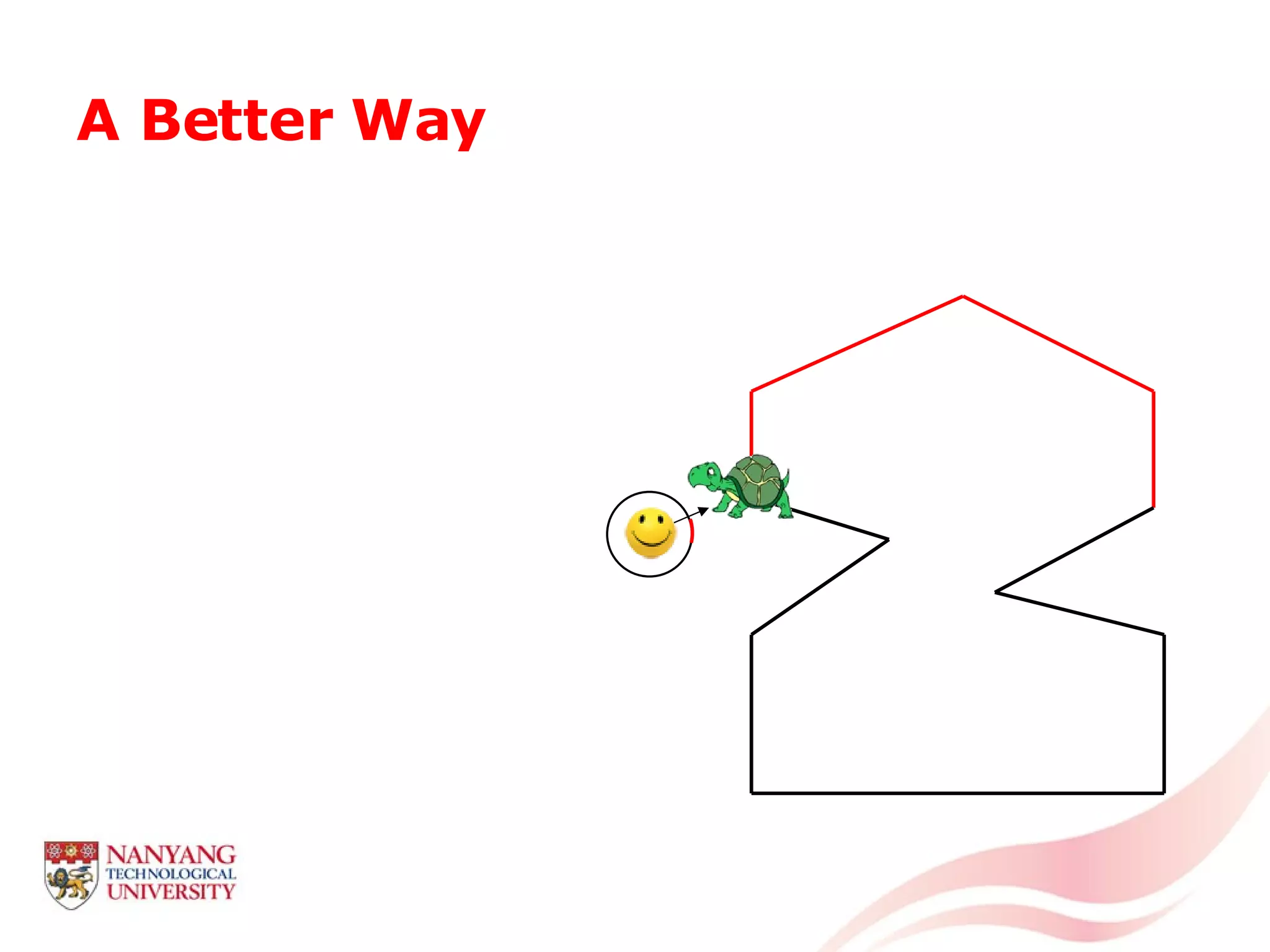


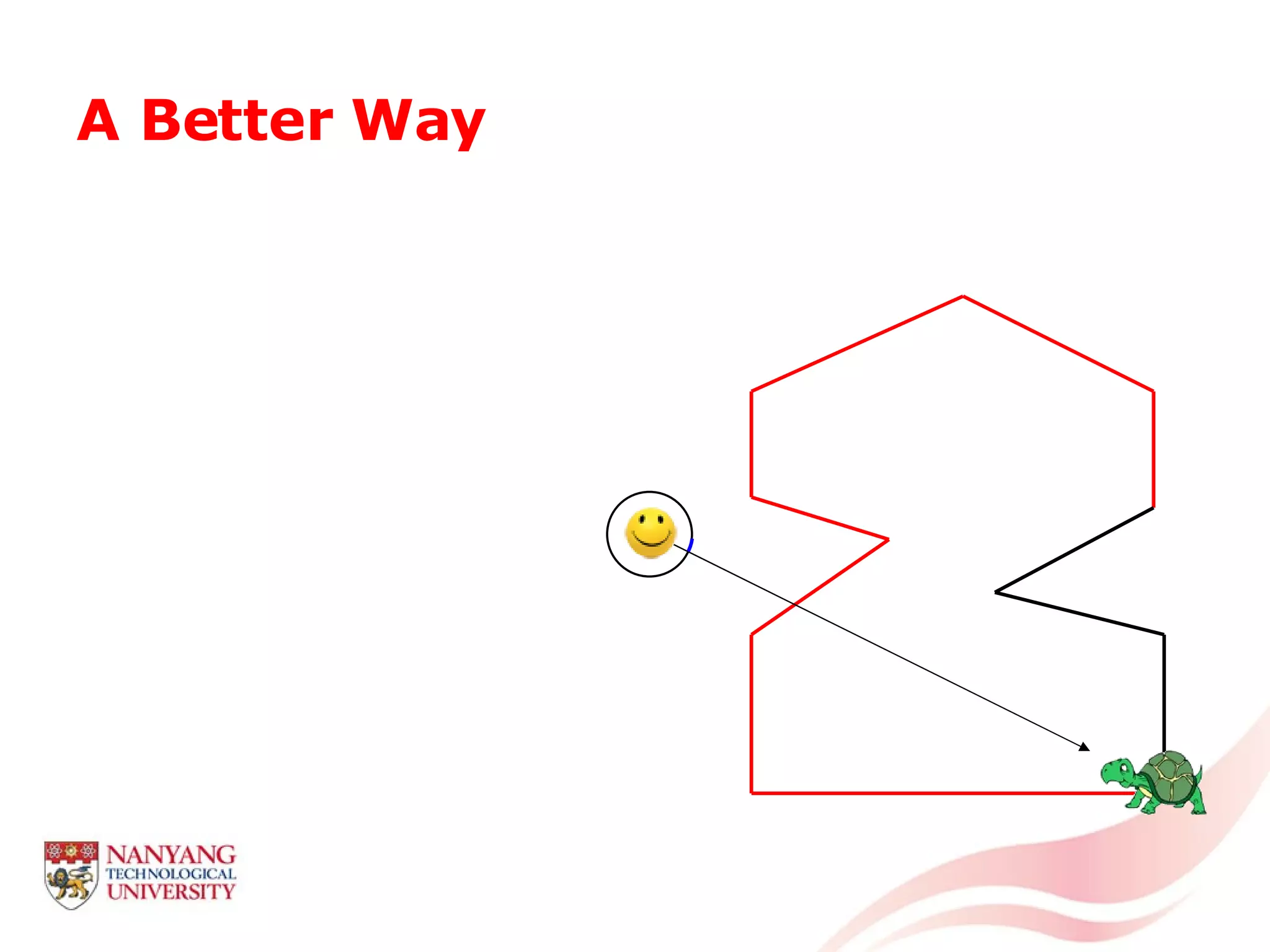

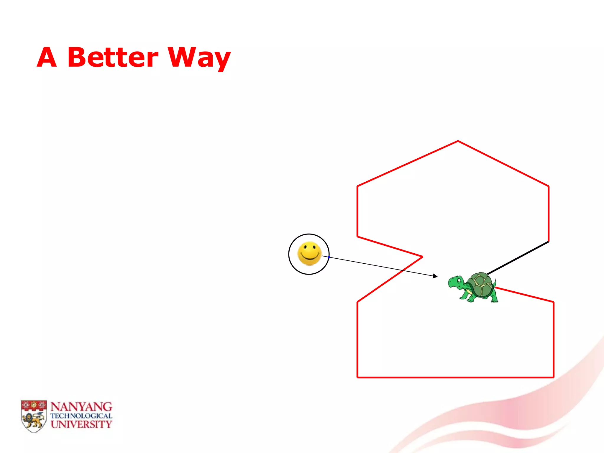


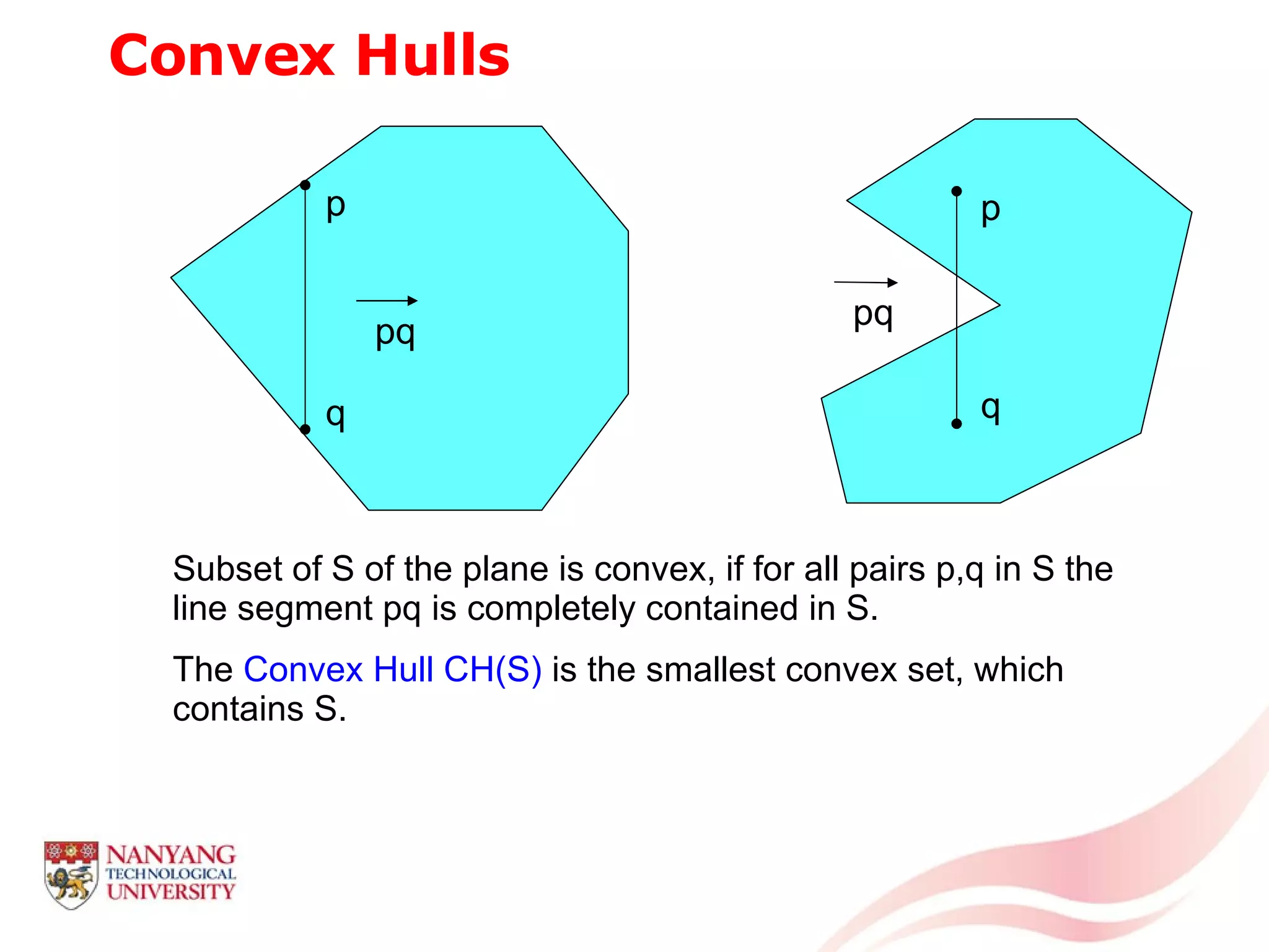
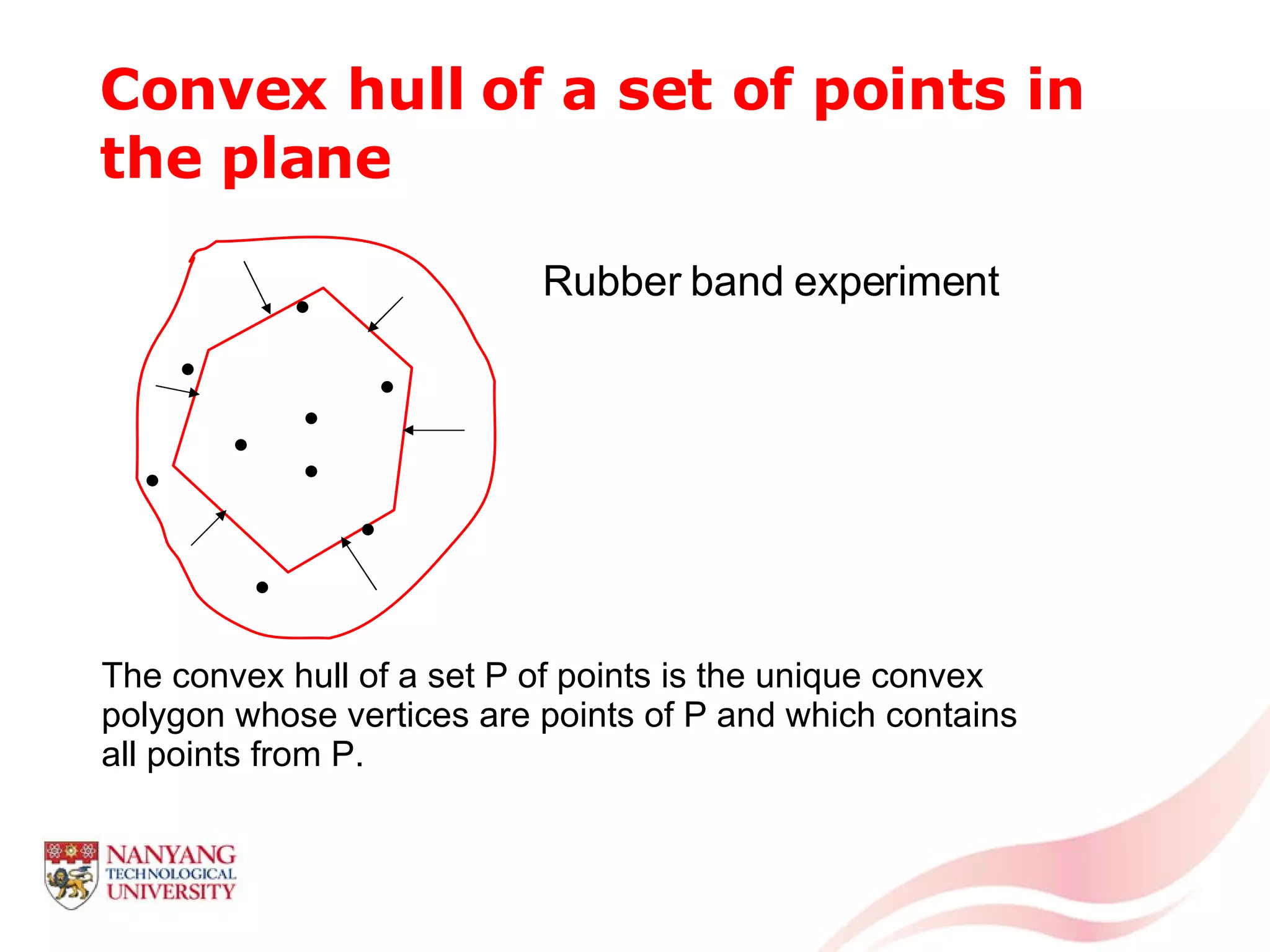
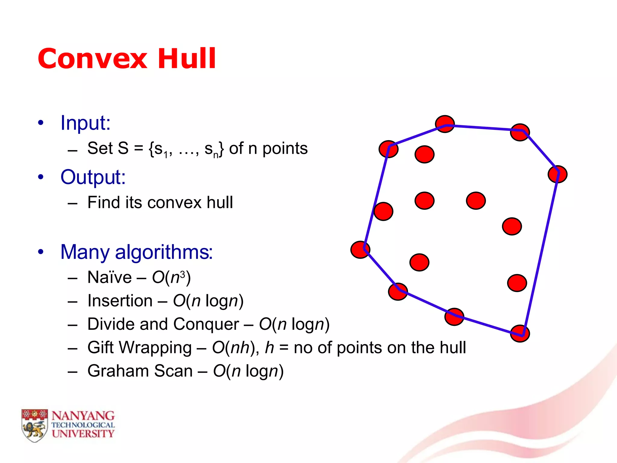
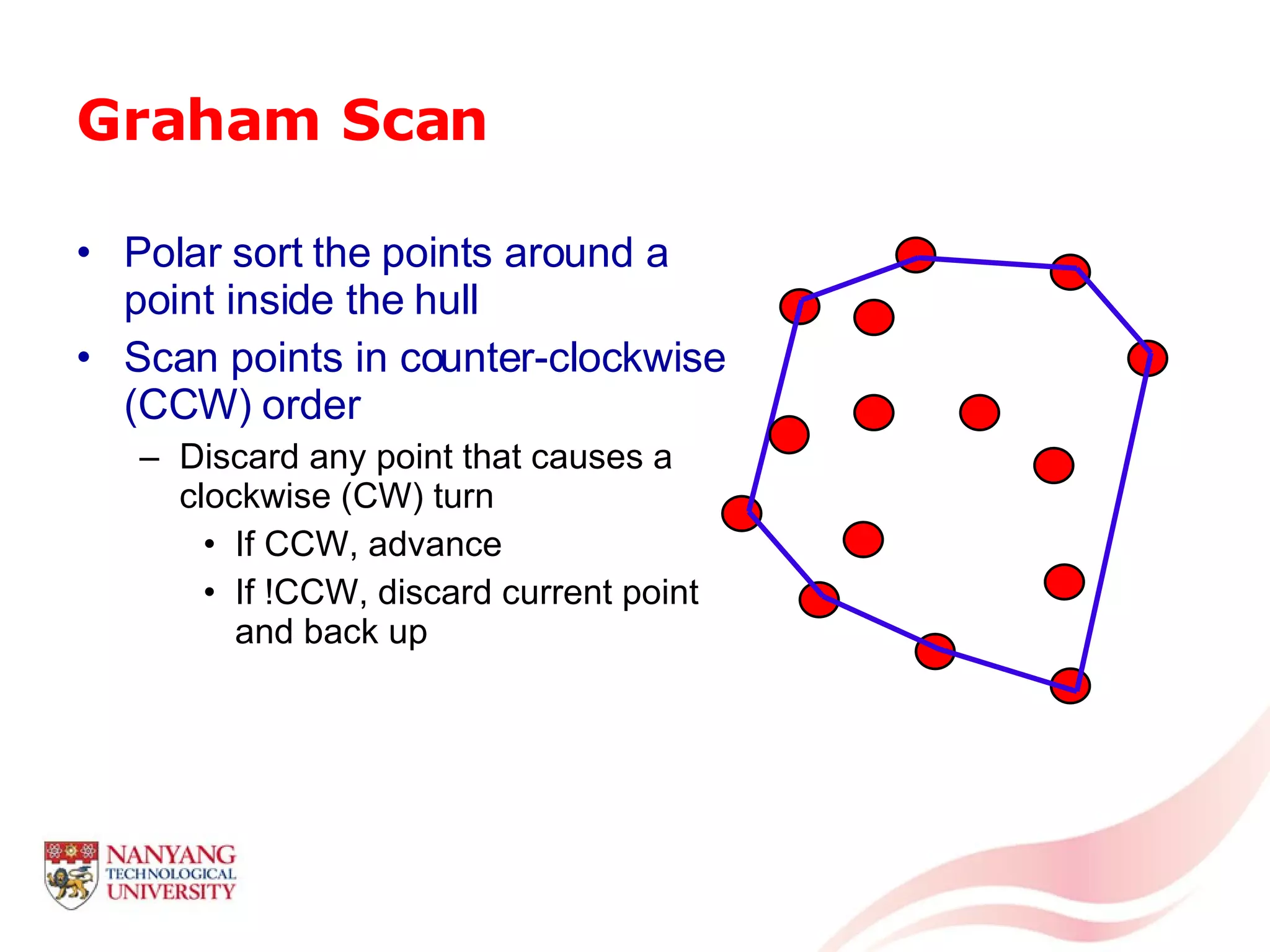
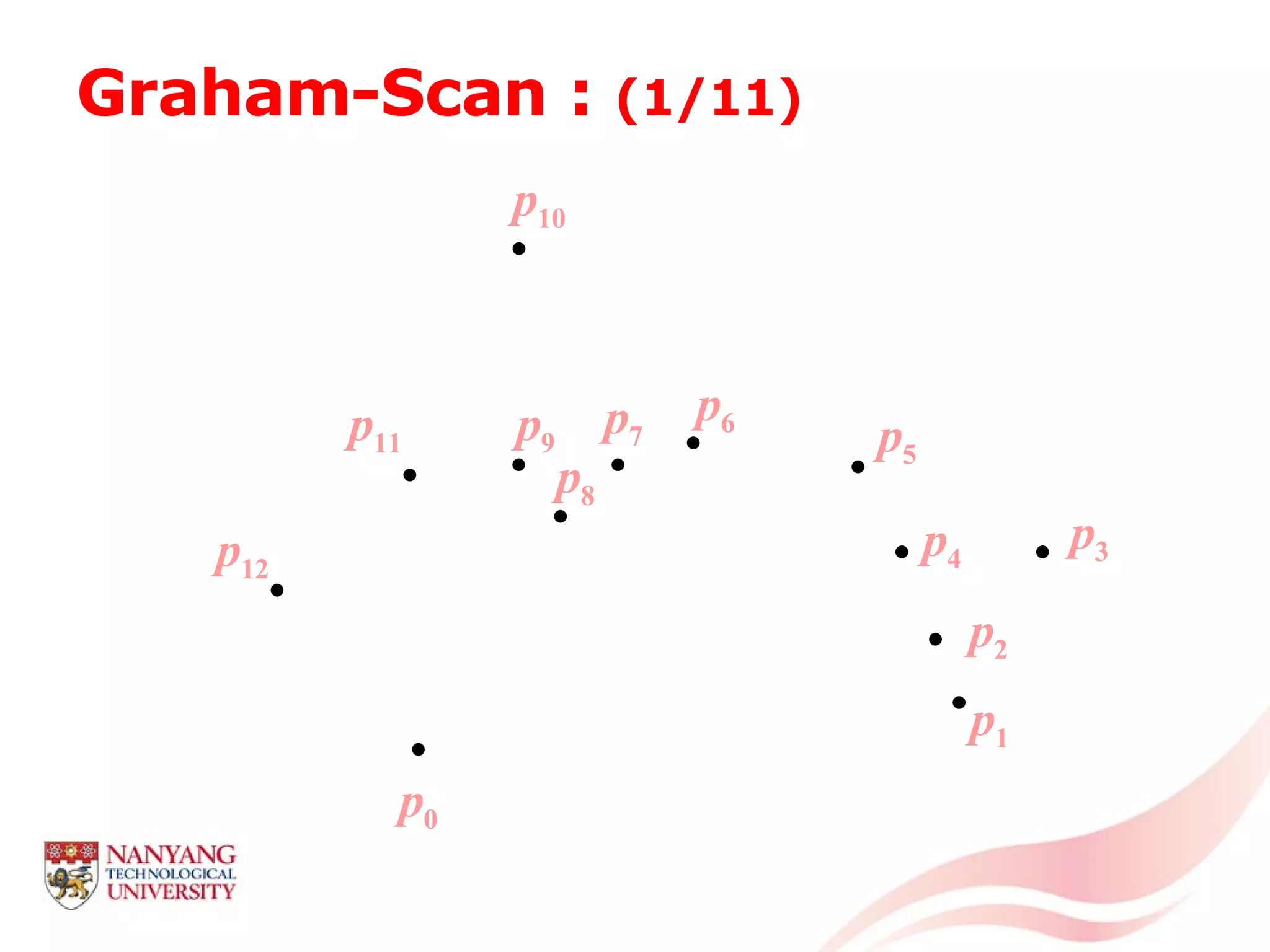
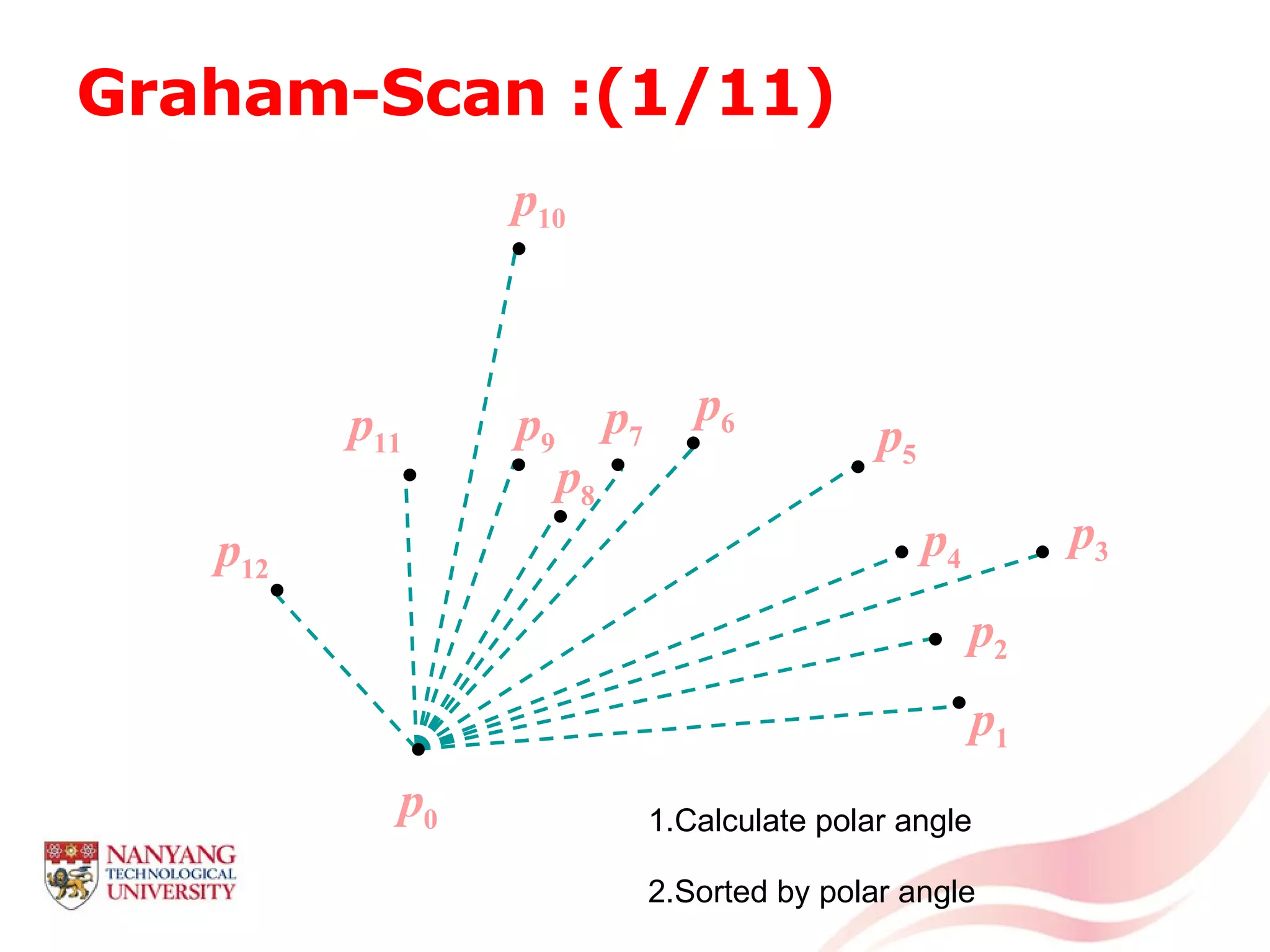
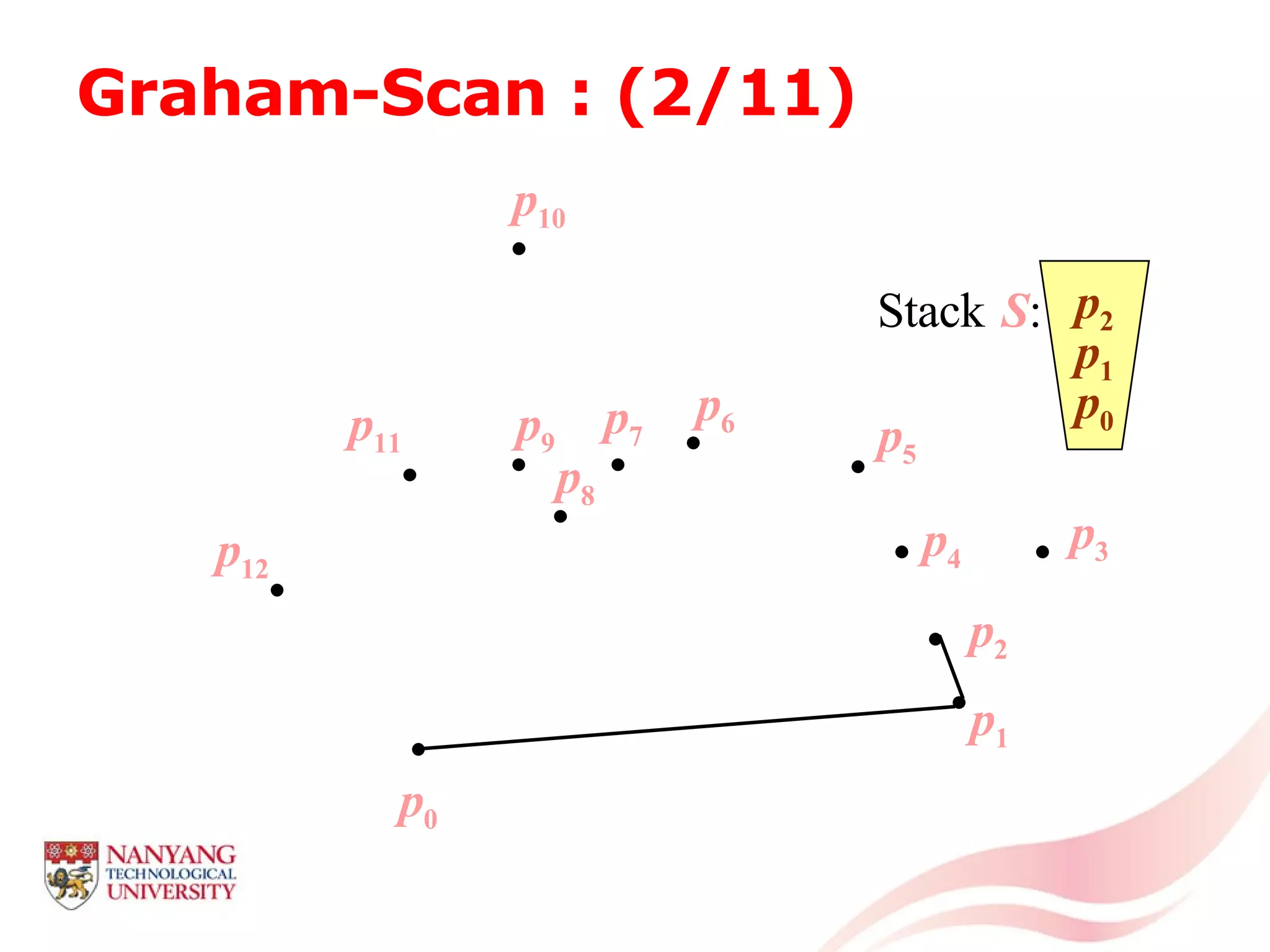
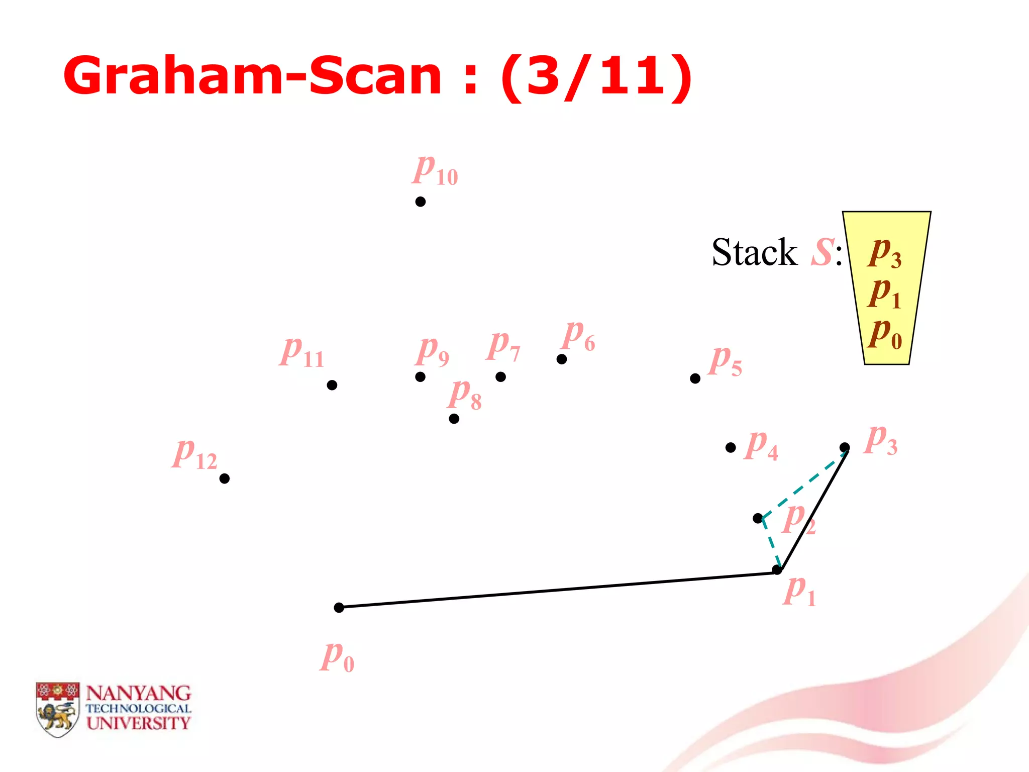
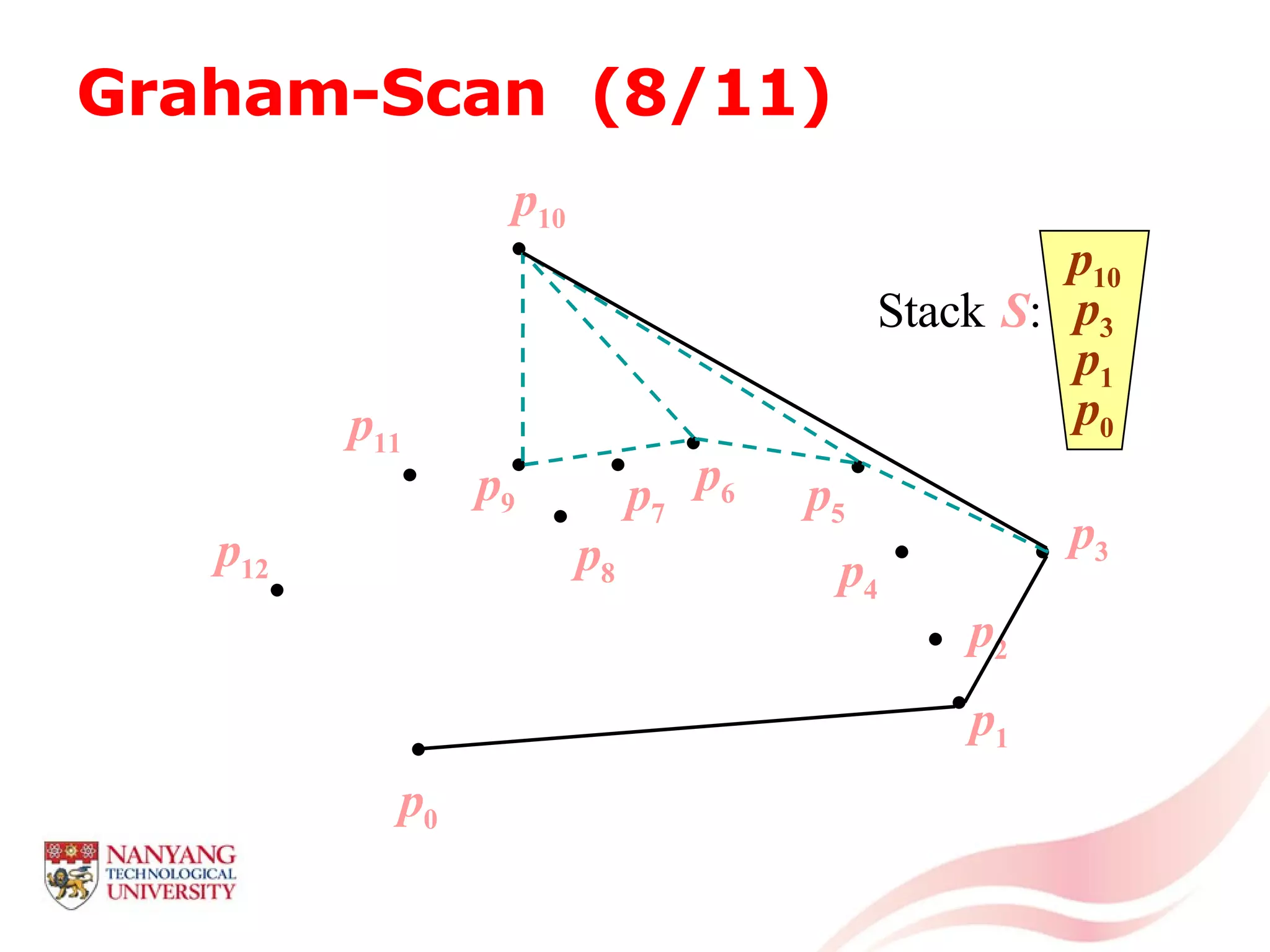
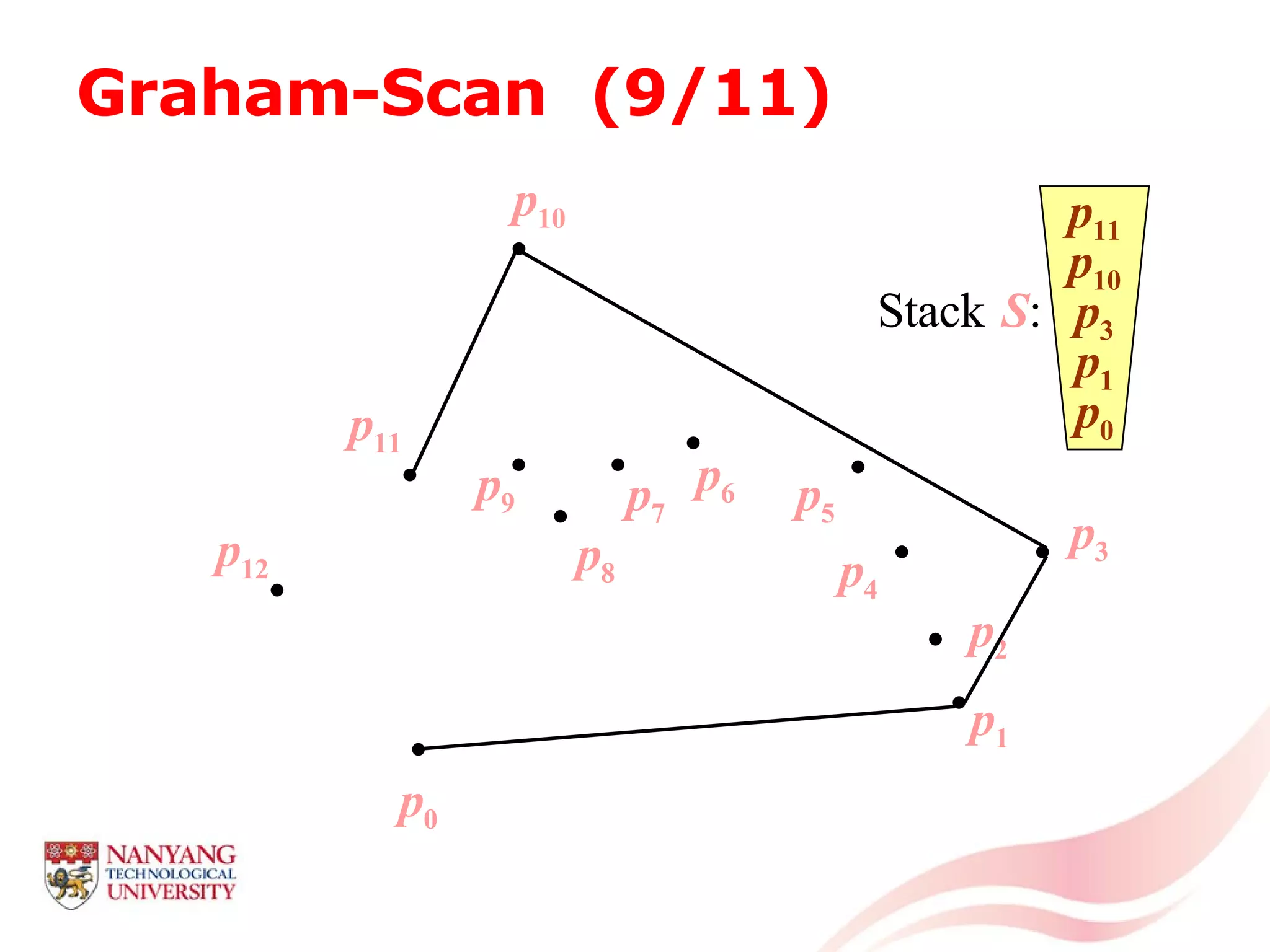
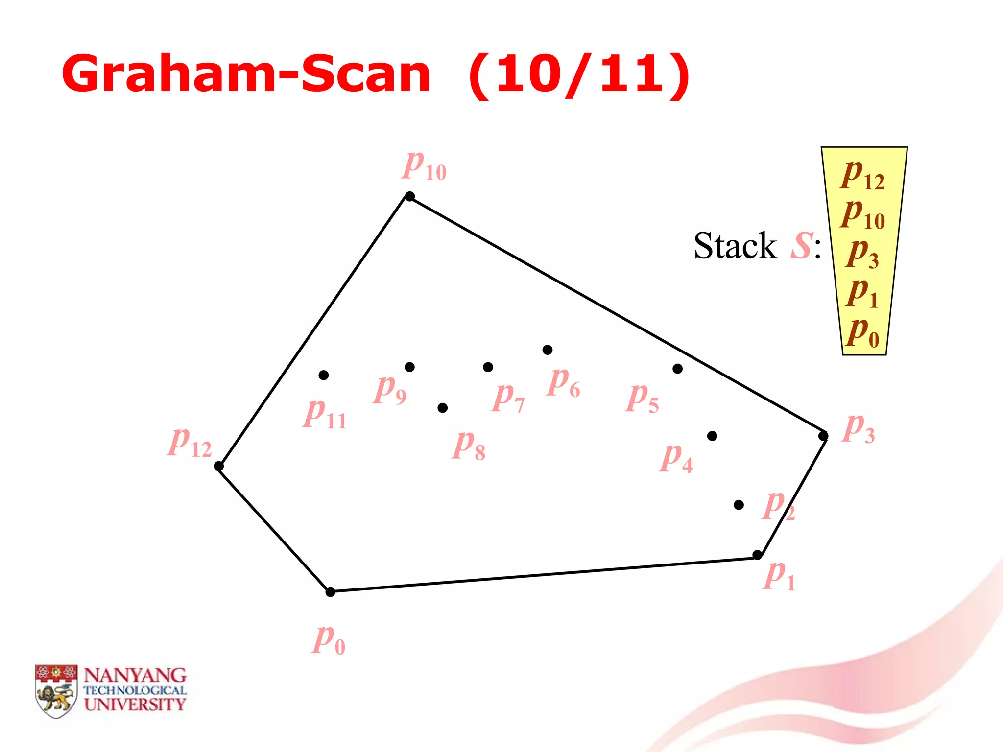
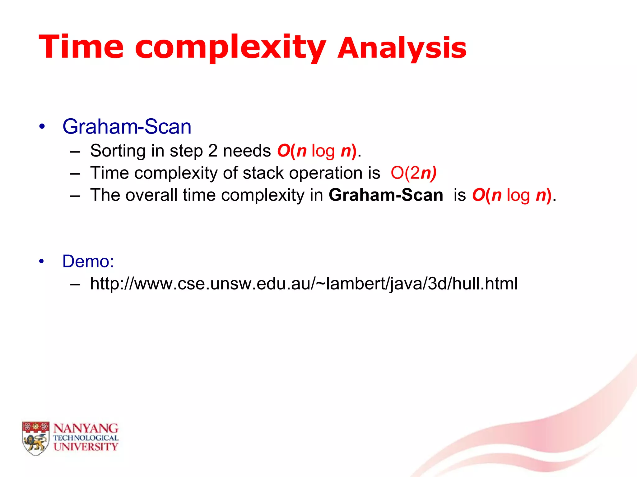

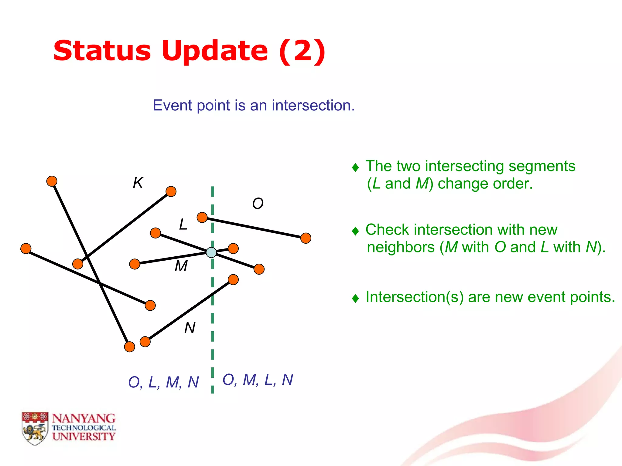
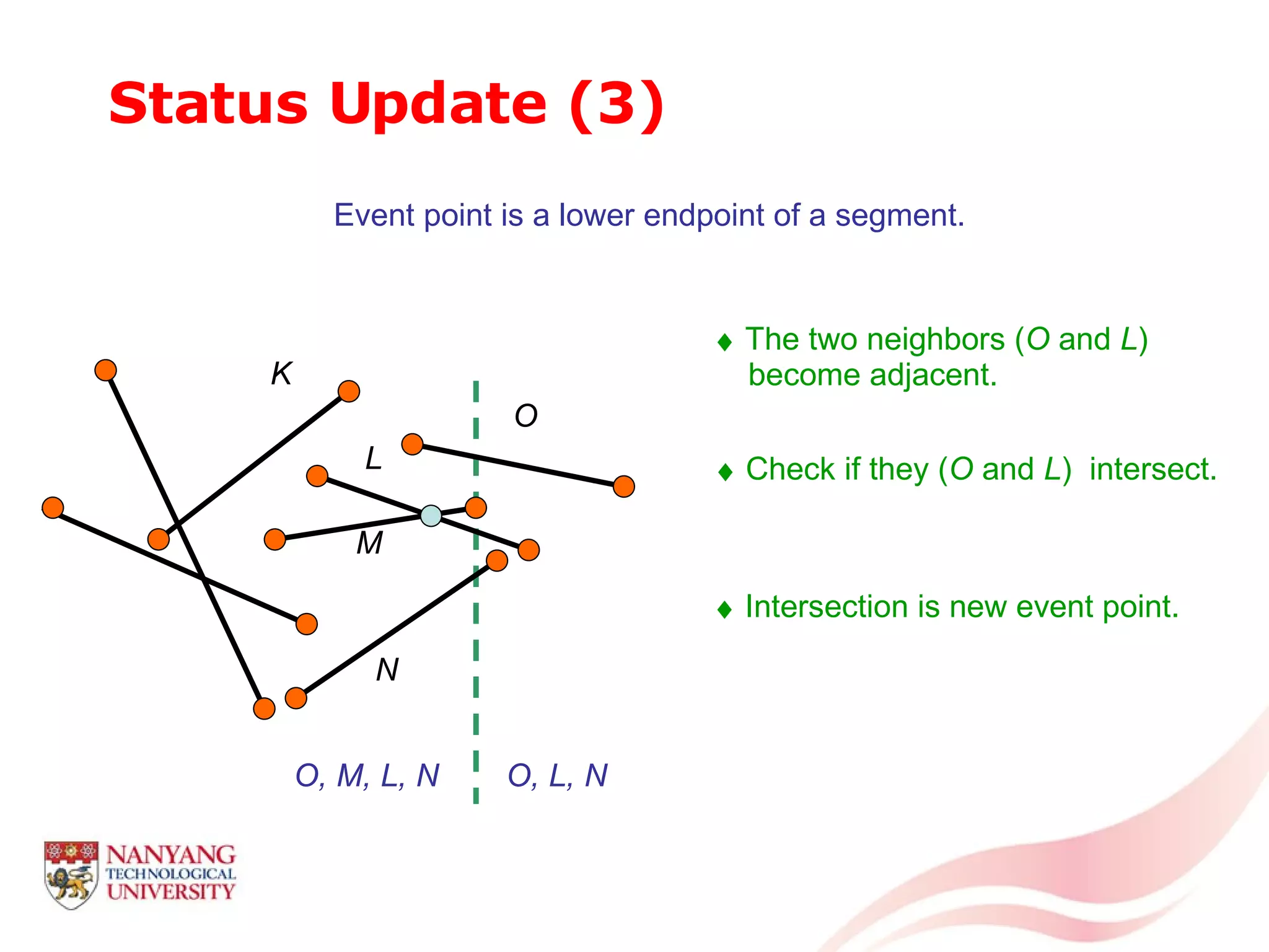
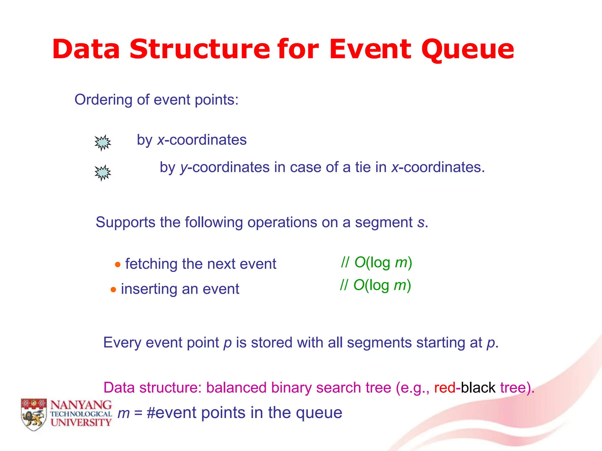
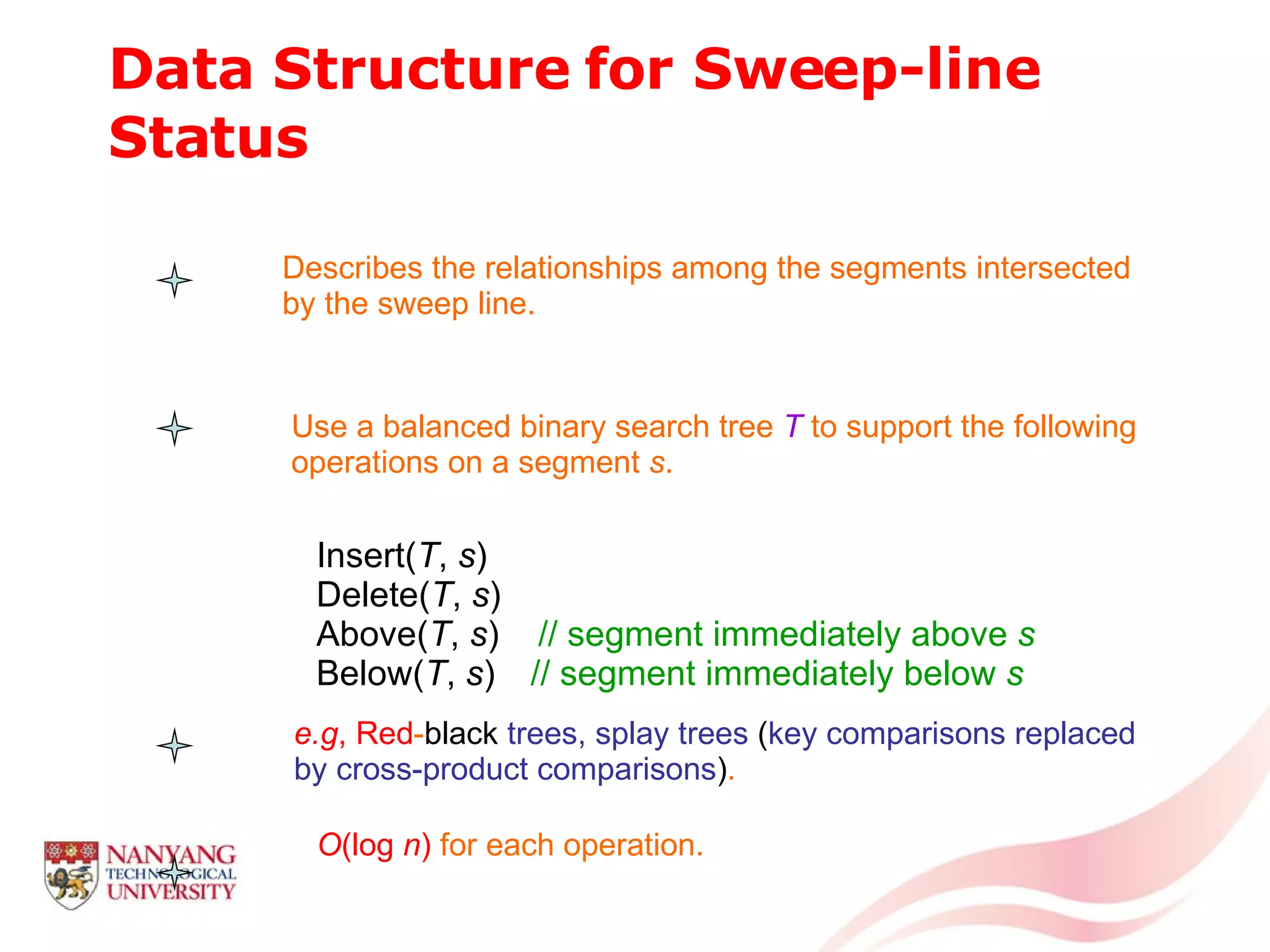
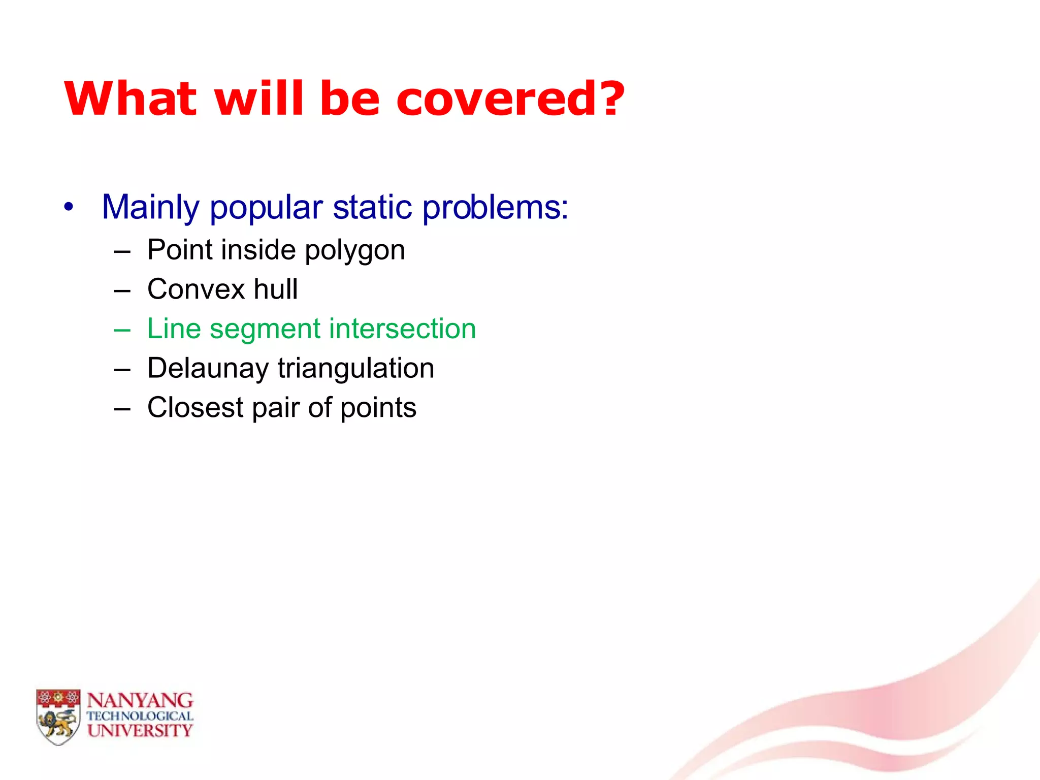

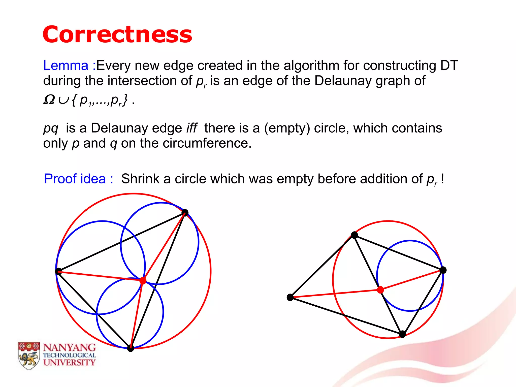
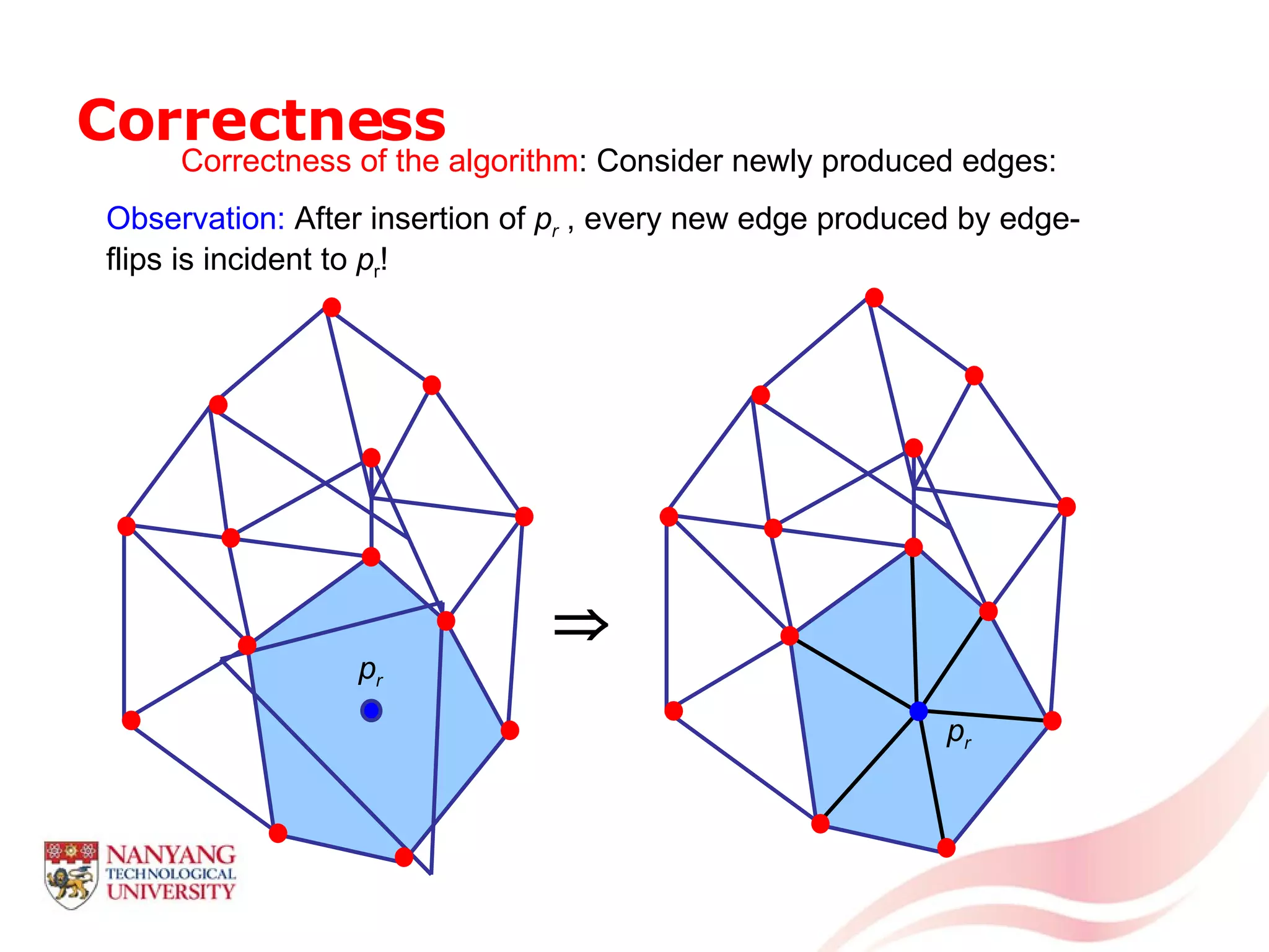
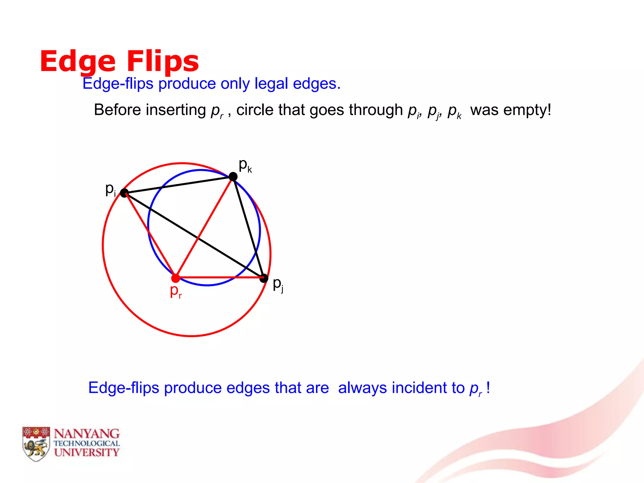
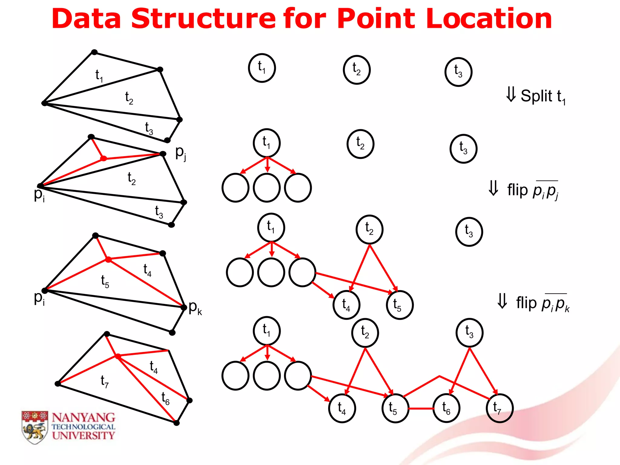


This document is a tutorial on computational geometry, covering key concepts such as point in polygon tests, convex hulls, line segment intersections, and Delaunay triangulation. It discusses various algorithms for finding convex hulls, managing line segment intersections, and generating triangulations while highlighting their complexities and advantages. The tutorial provides detailed examples and explanations for each method, catering to the needs of students and professionals in computer engineering.