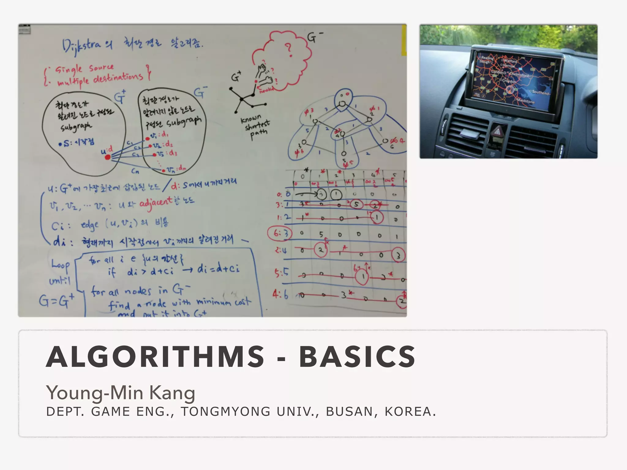
Download as PDF, PPTX
![BINARY SEARCH • Rules • your key: k • you know value v at i: array[i] = v • if k=v you found it • if k>v the left part of array[i] can be ignored • if k<v the right part can be ignored • Algorithm • 1. compare key and the middle of the list • 2. • if matched return the index of the middle • if not matched remove the left or right from the middle in accordance with the rule above rules • 3. goto 1 while the list is remained](https://image.slidesharecdn.com/algorithmssummary-140611015001-phpapp02/75/Algorithms-summary-English-version-19-2048.jpg)

![GRAPH TRAVERSAL • Depth-first vs. Breadth-first search • stack vs. queue A B C D E F G H I DFS Stack [A] [AB] [ABC] [AB] [ABD] [ABDE] [ABDEF] [ABDE] [ABDEG] [ABDEGH] [ABDEG] [ABDGI] Traversal: A, B, C, D, E, F, G, H, I BFS Queue Traversal: A, B, C, D, E, G, F, H, I [A] [B] [CD] [D] [EGH] [GHF] [HFI] A B C D E F G H I A B C D E F G H I DFS tree BFS tree](https://image.slidesharecdn.com/algorithmssummary-140611015001-phpapp02/75/Algorithms-summary-English-version-32-2048.jpg)
![STRING SEARCH RABIN-KARP METHOD • Rabin-Karp • T: text with size of m characters • p: pattern with n characters • h = hash(p) • hi: hash value of n-character substring of T starting at T[i] • if h = hi, string “T[i]…T[i+n-1]” can be p • i=0 to m-n • Hash hi = n 1X j=0 T[i + j] · 2n 1 j hi+1 = hi T[i] · 2n 1 + T[i + n] abcdefghijklmnopqrstuvwxyz hash value = h1 hash value = h2 h2 = h1 b · 210 + m](https://image.slidesharecdn.com/algorithmssummary-140611015001-phpapp02/75/Algorithms-summary-English-version-35-2048.jpg)

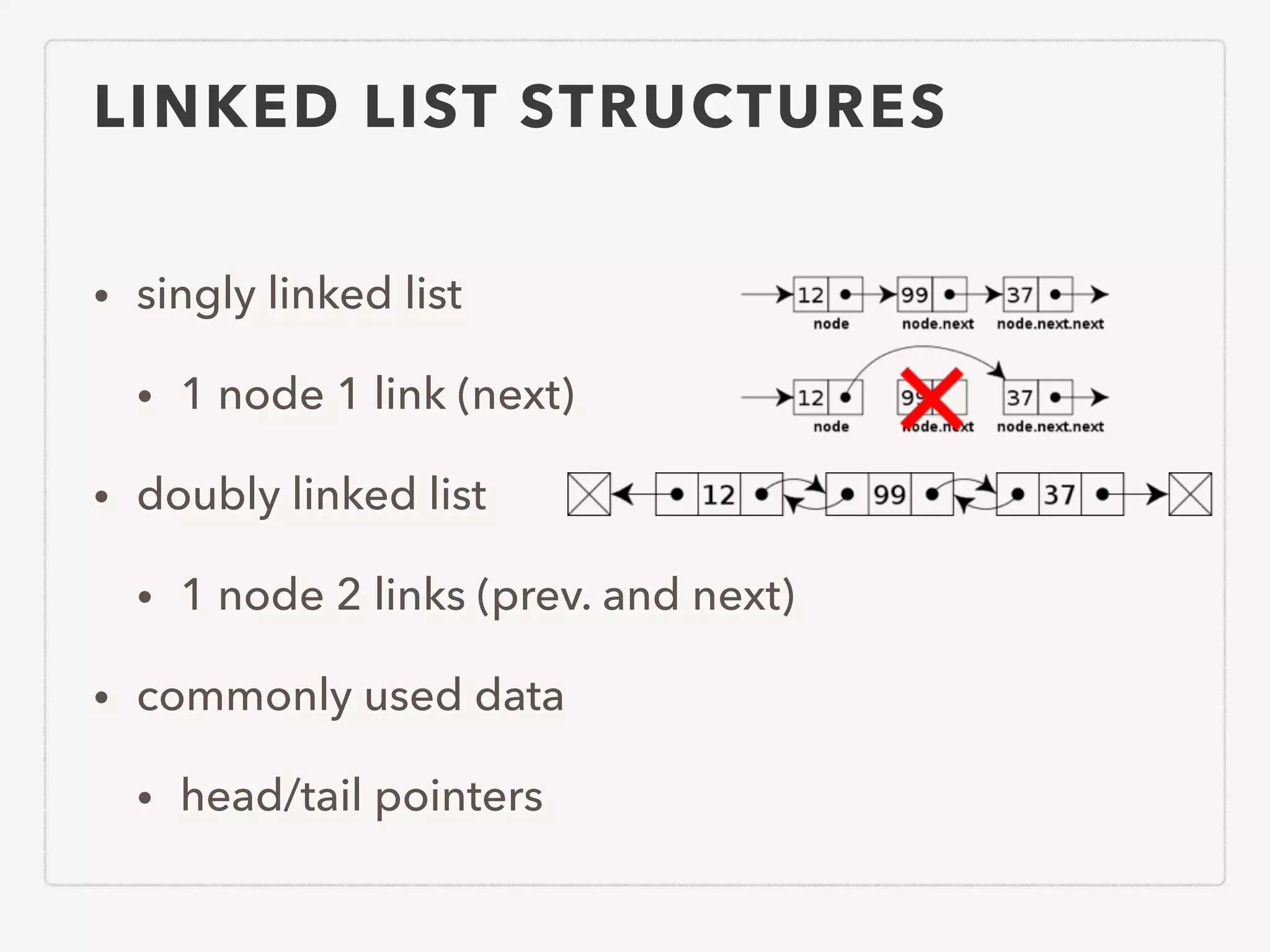
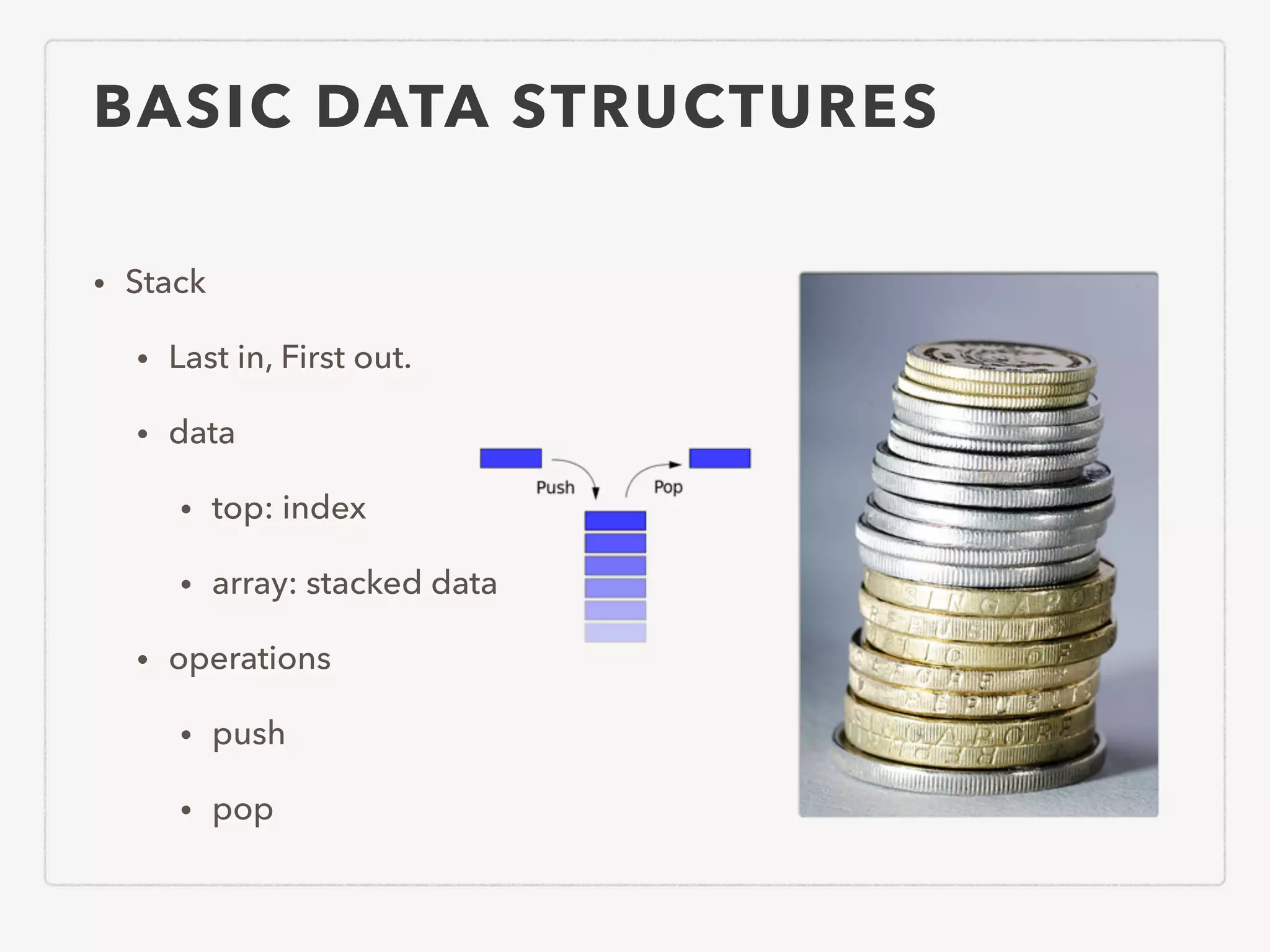
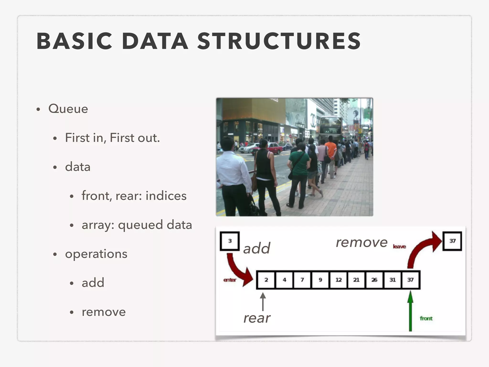
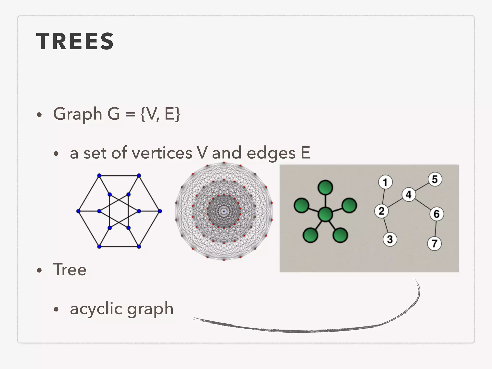
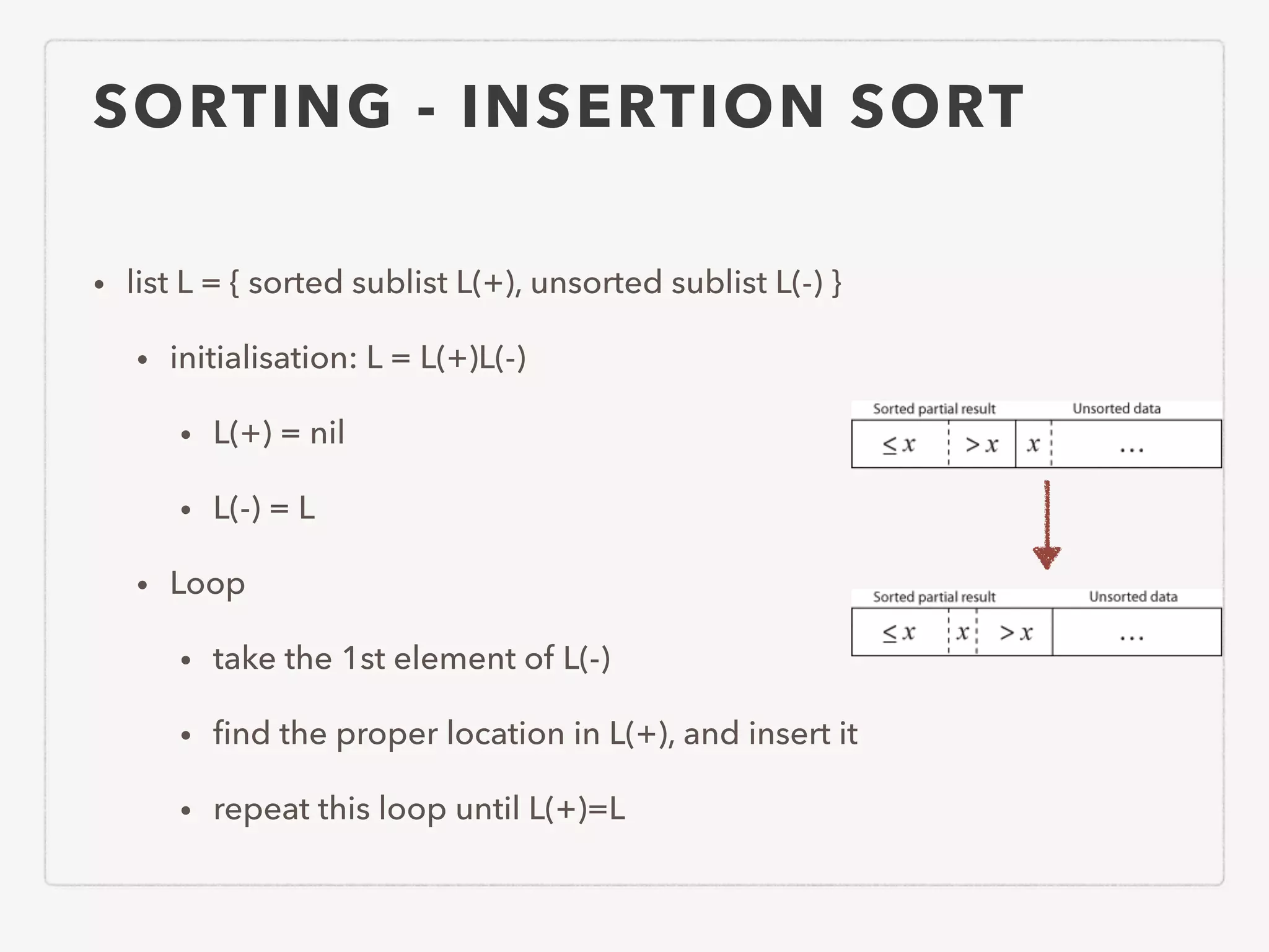
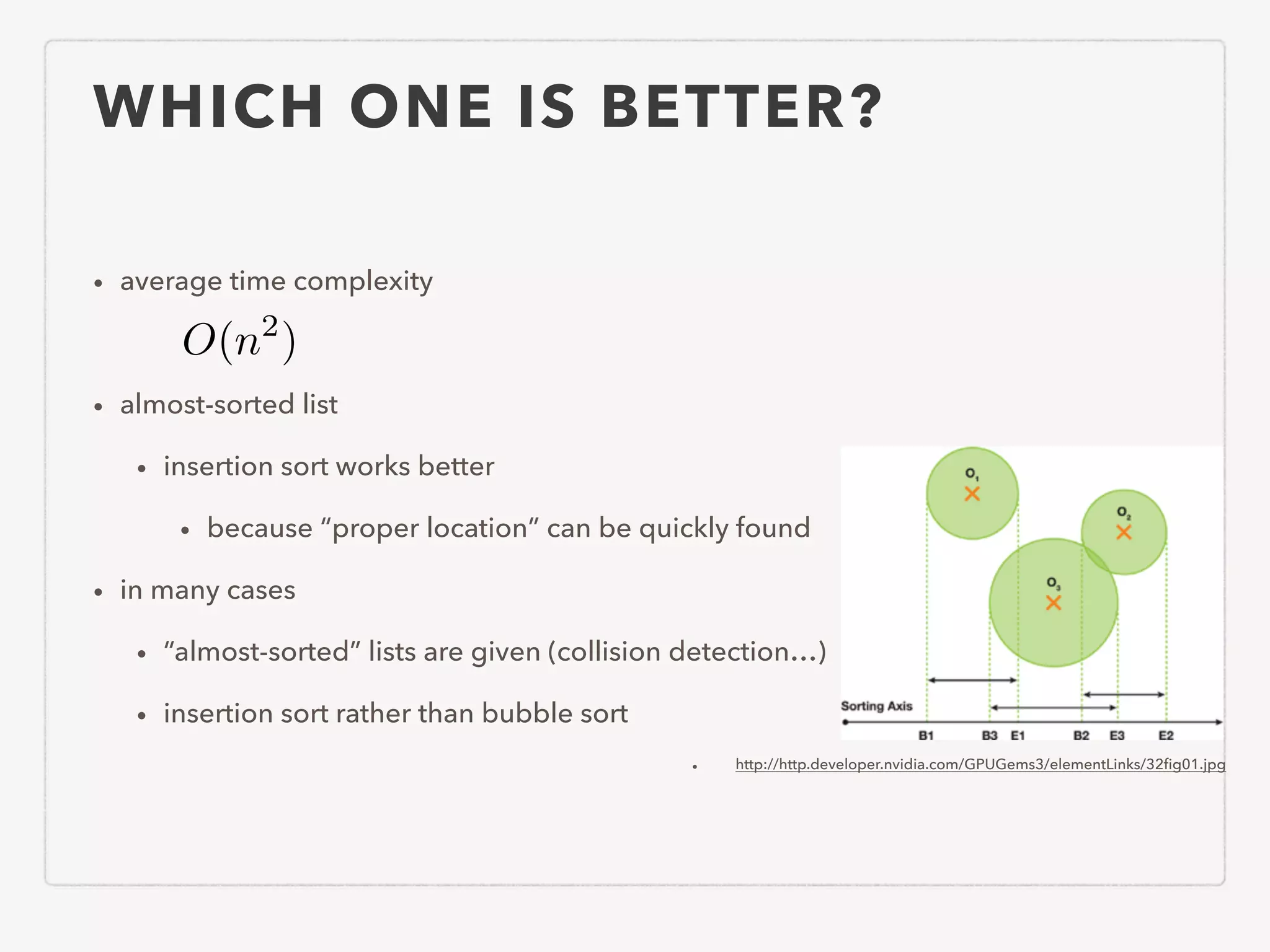
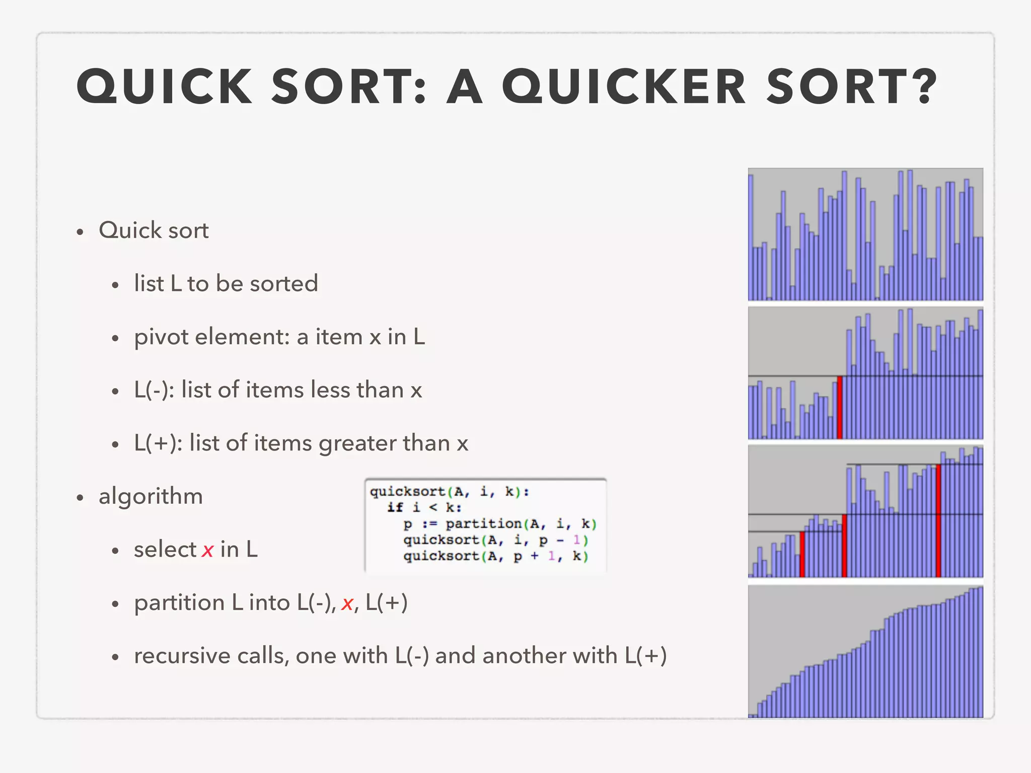
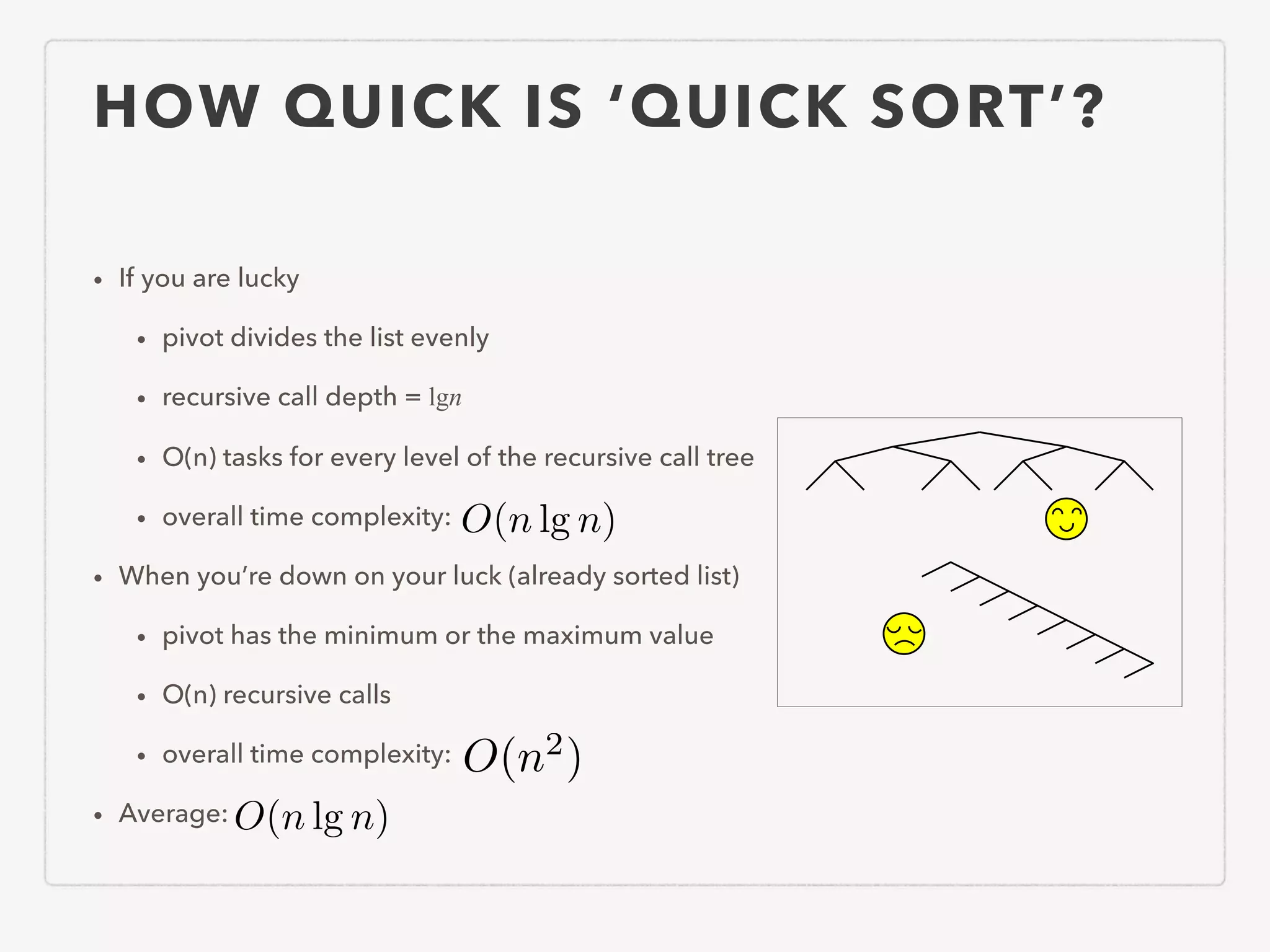
This document provides an overview of common algorithms and data structures. It begins by defining an algorithm and discussing algorithm analysis techniques like asymptotic analysis. It then covers basic data structures like arrays, linked lists, stacks, queues, and trees. It explains various sorting algorithms like selection sort, bubble sort, insertion sort, quicksort, and mergesort. It also discusses search techniques like binary search and binary search trees. Other topics covered include priority queues, hashing, graphs, graph traversal, minimum spanning trees, shortest paths, and string searching algorithms.