The document is a compilation of programming assignments designed for a digital image processing course at Sharif University, focusing on implementing tasks using Python and OpenCV. It includes installation guides for required software, detailed assignment breakdowns, and goals for students to enhance their skills in image processing. The content emphasizes hands-on learning with gradual difficulty and provides codes and resources to facilitate the learning process.


![Problems Question 1: Implement Kronecker product between two matrices. The only library you are allowed to use is Numpy. You should complete the method kron, in the module named ‘math’ which is placed under the package ‘ipl_utils’. We imported this module in the file named ‘q1.py’ and prepared some code for you to complete. 1. We have defined 4 pairs of numpy variables. Some of them are initialized to None. Please make changes to the code and initialize them as the comments say. You can use this link to sample from a Normal distribution using numpy. 2. Compute the Kronecker products of each pair using ipl_math.MatrixOperations.kron 3. Compute the Kronecker products of each pair using numpy.kron. Related docs can be found here. 4. Use assert statements to make sure your function has computed the true values. In the case of floating point matrices, the assertion may fail due to different implementations of your function and Numpy’s. In order to fix this, first convert your floating point matrices to integer ones. There is a sample line of commented code there in the python file provided. We used the astype method in order to do this. You have to perform the said step regardless, whether the assert statement works fine with or without it. Question 2: Read all of the images in the folder ‘q2_images’ using OpenCV’s function imread and a for loop. imread gets a numpy array. Code in the ‘q2.py’ file. 1. Store all of these arrays in a python list. 2. In python jargon, we call a .py file which contains class and function implementations, a ‘module’. Create a module and name it interpolate.py under the ‘ipl_utils’ package. In that module, write a function named avg_interpolate which takes a Numpy array as an image, does interpolation on it and then returns it. This function must scale the width of the image by 2. You can use the average of two nearest pixels for interpolation. Be sure to check the results, and see if you have not scaled the height instead of the width. Use this function in the ‘q2.py’ file. Question 3: In this problem, we want to take Fourier transform of an image, apply a low-pass filter to it and then take the inverse Fourier transform to get the manipulated image. You can use this tutorial as a baseline for your implementation. Read all of the images in the folder ‘q3_images’ using OpenCV’s function imread and a for loop. Code in the ‘q3.py’ file. 1. Apply low-pass filters which preserve 1/10, 1/5 and 1/2 of the whole range of frequencies of each one of the axis you have. Then apply inverse Fourier transform to see what happened to the image. You must have 3 results. 2. [Extra points] We have provided a file named ‘trackbar.py’ for you. Run it and see what happens. Here is where we found this code. Use this code as a baseline. Write a code that computes what percentage of the frequency range must be preserved from the trackbar’s value. Then take inverse Fourier transform and show the image below the trackbar. Question 4: Use the red channel of the image ‘give_red.jpg’ to be the red channel of the image ‘base.jpg’ and save the result into a file. Code in the ‘q4.py’ file.](https://image.slidesharecdn.com/practicalall-191006194716/75/A-Hands-On-Set-of-Programming-Problems-Using-Python-and-OpenCV-13-2048.jpg)
![• [Extra points] As you may have noticed, by changing the red channel for the whole base.jpg image we have altered its color to something else. Can you devise a method that outputs the same result, but preserves the true color of ‘base.jpg’ where there is no track of ‘give_red.jpg’? We have not considered any specific right answer for this question, and we wait to see your innovations.](https://image.slidesharecdn.com/practicalall-191006194716/75/A-Hands-On-Set-of-Programming-Problems-Using-Python-and-OpenCV-14-2048.jpg)

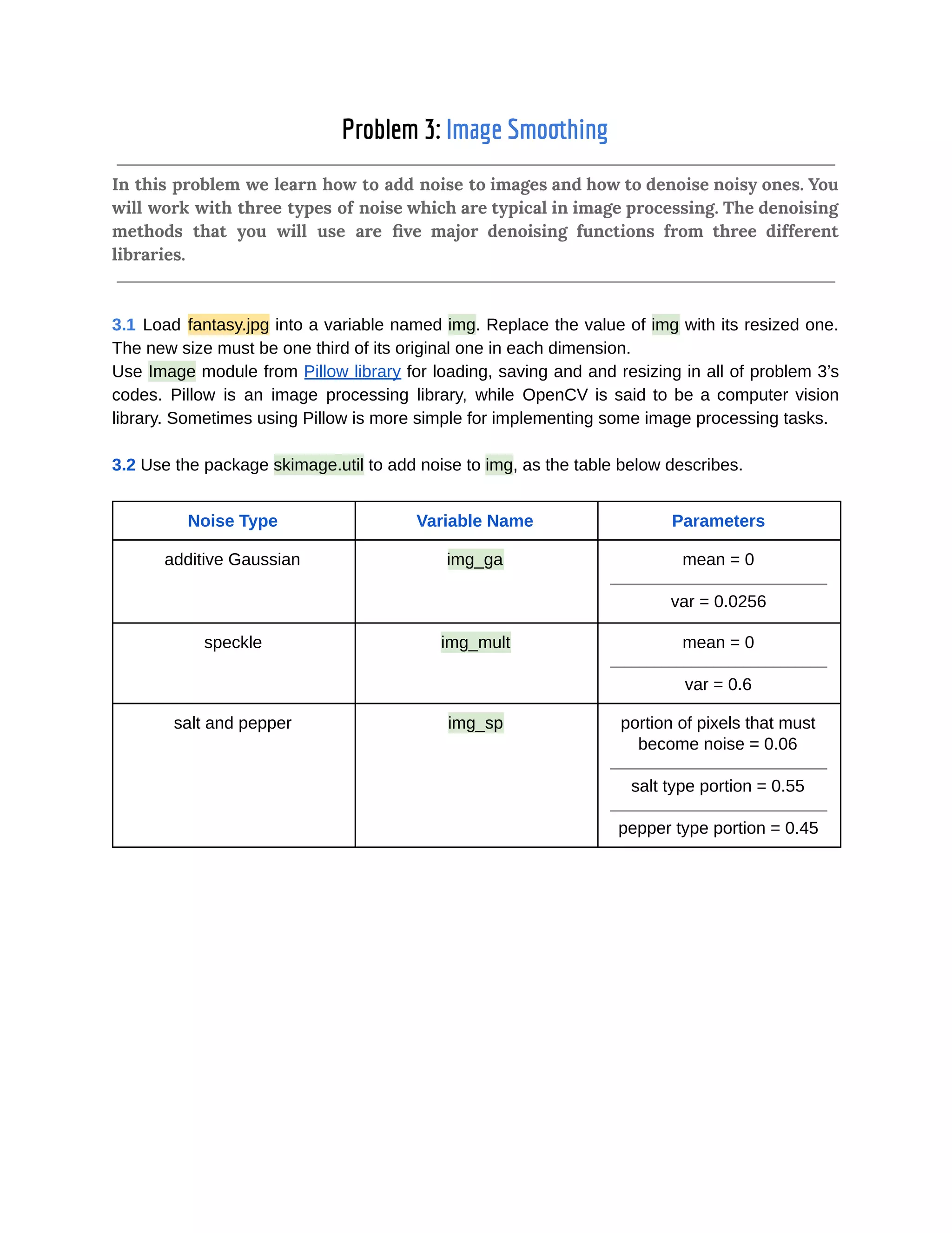
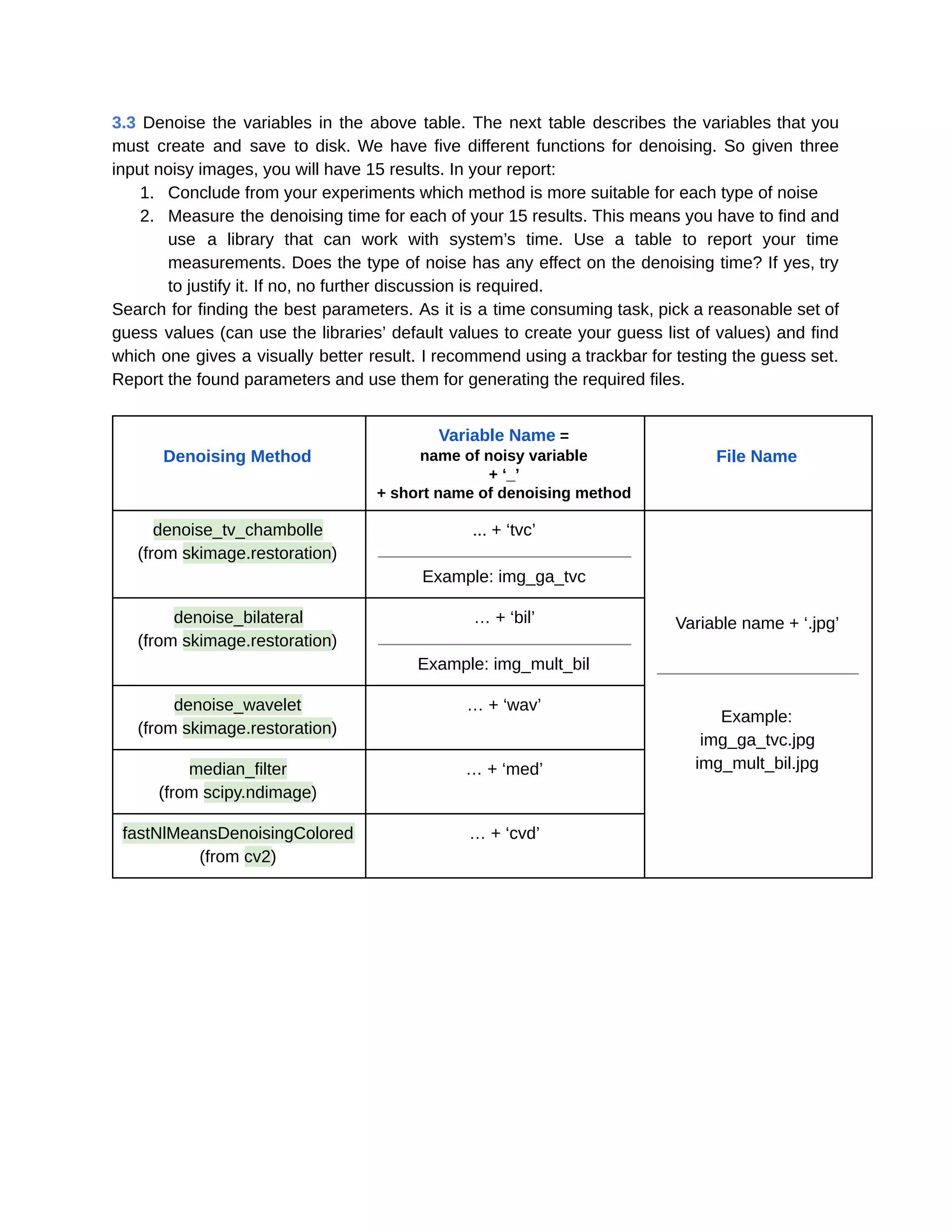
![10/6/2019 hw2_practical - Google Docs https://docs.google.com/document/d/17CCDela47Kj8xPsKAKVYUr8Iw7siRWGDmLsQo1-XAJg/edit 2/5 Problem 1: histogram equalization and color spaces In this problem, we want to enhance an image of brain in grayscale color space. We will also work on enhancing a color image of stellar winds, which is taken by Hubble space telescope! 1.1. Open p1.py. Load the image named brain.jpg into a variable named brain_light, brain_darker.jpg into brain_dark, nasa.jpg into nasa_colored. Brain_light and brain_dark must be in grayscale space, and nasa_colored must be in RGB space. Note: OpenCV’s method imread gives BGR images by default. 1.2. Write a function hist_eq(img) that takes a two dimensional matrix as a grayscale image, enhances it by histogram equalization and returns it. 1.3. Use hist_eq function to enhance the three images. For nasa_colored, hist_eq each of its three channels separately and save the result into a variable named nasa_separate. 1.4. Change the color space of nasa_colored and save it in a new variable named nasa_hsv. Use hist_eq on the Value channel only, convert it back to RGB and save it into a variable named nasa_enhanced. 1.5 Save the data that table below describes. By ‘brain_x’ in the table, we want you to change ‘x’ to ‘light’ or ‘dark’. Your report must at least cover these points: ● How does CDF graphs look like after applying hist_eq and whether that follow the theory of histogram equalization. ● Compare the results of brain_dark and brain_light. Justify your answer. ● Briefly talk about HSV color space, its usages and why it’s suitable for this problem. ● Explain the difference between nasa_enhanced and nasa_colored. Data File name Histogram of the original image brain_x_hist_org.jpg [example: brain_dark_hist_org.jpg] Histogram after applying hist_eq brain_x_hist_eq.jpg CDF of the original image brain_x_cdf_org.jpg CDF after applying hist_eq brain_x_cdf_eq.jpg Enhanced brain_light brain_light_enhanced.jpg Enhanced brain_dark brain_dark_enhanced.jpg Enhanced nasa_colored, each RGB channel separately nasa_separate.jpg Enhanced nasa_colored, using HSV nasa_enhanced.jpg 2](https://image.slidesharecdn.com/practicalall-191006194716/75/A-Hands-On-Set-of-Programming-Problems-Using-Python-and-OpenCV-16-2048.jpg)


![10/6/2019 hw3_practical - Google Docs https://docs.google.com/document/d/1mGFJnykAkaKwbdnM6xXCmwXTIneMBy5SZKW8B7MatF4/edit 3/6 Problem 1: Morphological Image Processing Functions In this problem, we use morphological image processing functions to understand what they can do for us. Using them we can find edges, skeletons of shapes, search for patterns and even sometimes remove the background from an image! 1.1 Load circles.png into a variable named circles. Find the boundary of circles by using morphological functions of OpenCV. You can not use cv.MORPH_GRADIENT. Instead, combine other functions to find the result. Load se_rad1.npy and se_rad4.npy which are structuring elements with radius 1 and 4 from the folder resources/numpy_files and use them, and save the result of using each. Check this link if you don’t know how to load a .npy file into a numpy array. 1.2 Find the skeleton of circles using skeletonize from the package skimage.morphology. 1.3 Load chess.npy into a variable named chess. It contains an image of a half chessboard. Perform the hit-or-miss transform on chess. se_hit and se_miss are two structuring elements defined below. se_hit must hit the pattern and se_miss must miss it. You can use ndimage.binary_hit_or_miss function from scipy package. How should the structuring elements be designed in order to detect the top left corner of all the white squares? se_hit se_miss [ [0, 0, 0], [1, 1, 0], [0, 1, 0], ] [ [0, 1, 1], [0, 0, 1], [0, 0, 0], ] 1.4 Load digits.png into a variable named digits.This image has a noisy background with varying illumination, so a little preprocessing before the main operations won’t hurt. Estimate the background of digits by morphological functions and store the result in a variable named bg. Ue bg to remove digits‘s background. Then apply thresholding to extract digits in a binary matrix form. In my case, there is something like salt and pepper noise in the image at this level. If you saw that noise too, use median_filter from scipy.ndimage, or other effective morphological functions to reduce that. Next, try to fix gaps or connected symbols in the digits, if there were any. The file digits_sample_solution.png contains the result of our solution for this problem. Try to be at least as good as that.](https://image.slidesharecdn.com/practicalall-191006194716/75/A-Hands-On-Set-of-Programming-Problems-Using-Python-and-OpenCV-22-2048.jpg)

![10/6/2019 hw4_practical - Google Docs https://docs.google.com/document/d/1IhvTrjDZn5v3E9d0-Dm2daSEMTNREVMwwLSreiQdOXE/edit 1/3 Assignment 4 [EXTRA POINTS] Due: Tir-Mah 19th, 1398](https://image.slidesharecdn.com/practicalall-191006194716/75/A-Hands-On-Set-of-Programming-Problems-Using-Python-and-OpenCV-26-2048.jpg)

![10/6/2019 hw4_practical - Google Docs https://docs.google.com/document/d/1IhvTrjDZn5v3E9d0-Dm2daSEMTNREVMwwLSreiQdOXE/edit 3/32 This assignment is about Image Style Transfer and Google’s Deep Dream. The main sources for answering the questions are the file ‘Style Transfer Using CNNs.pdf’ in your assignment folder and this Google AI Blog post. [+0.1] 1. Write one or two paragraphs about what Deep Dream is and how it works. Explain the problem statement and its solution. You don’t need to include math. Try to be smooth and clear. [+0.1] 2. Get the code of Neural Transfer from this link. Find a pair of new input images from the internet and run the code. Save and report your results. Try to get an acceptable output here, since this algorithm is not suitable for combining some images. [+0.1] 3. Explain why Gram matrix works as a good measure for capturing the style of an image. [+0.2] 4. Find a creative and new way of generating images using fixed and pre-trained Neural Networks as feature extractors. You don’t need to implement your idea, but you have to justify it and state why do you think it works. [+0.5] 5. Find a new function of a layer of a Neural Network’s features that is suitable for style extraction. Implement this function and produce the output using images that you downloaded for problem 2. Report and justify your results.](https://image.slidesharecdn.com/practicalall-191006194716/75/A-Hands-On-Set-of-Programming-Problems-Using-Python-and-OpenCV-28-2048.jpg)