Solve Deep-ML Problems (Part 1) — Machine Learning Fundamentals with Python

Author(s): Jeet Mukherjee

Originally published on Towards AI.

In this article, we’ll explore how to code five machine learning concepts using Python. We’ll fetch the problem statement along with starter code from Deep-ML. Additionally, I’ll be adding a little theory with each problem to give you an idea behind the code.

5 Machine Learning Concepts

1. PCA (Principal Component Analysis)
2. Feature Scaling
3. Confusion Matrix for Binary Classification
4. Overfitting & Underfitting
5. Random Shuffle of Dataset

PCA (Principal Component Analysis)

Principal Component Analysis is a dimensionality reduction technique. Let’s assume I have a dataset that contains n-1 independent features and 1 dependent feature. Now, this gives me an n-dimensional dataset, which in some cases might be very large. So, the dimension reduction technique can be used here to get only important features(columns), also known as components.

An important thing to keep in mind is that the loss of information should also be minimal while choosing only the important components.

Steps in PCA —

1. Data Standardization — It is crucial, as PCA chooses the important components that maximize the variance in data, so if the data isn’t standardized, PCA will be biased towards the features with a large numerical range.
2. Covariance Matrix — The next step is to compute the covariance matrix. It shows how features vary from each other.
3. Eigenvalues and Eigenvectors — Eigenvectors indicate the direction of the principal components, while eigenvalues describe the variance of each component.
4. Sort Eigenvalues and Eigenvectors — Rank the principal components in descending order of their eigenvalues. The first component explains the most variance, the second explains the next most, and so on.
5. Return TopK Components — Finally, return the top K components as new features(principal components).

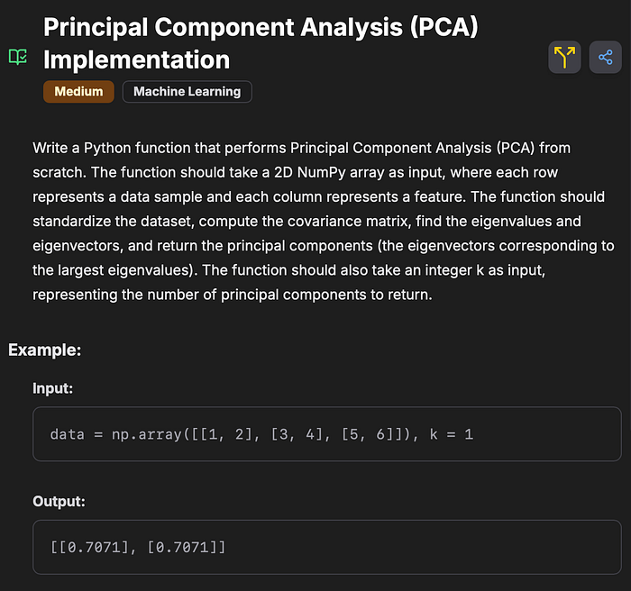
Problem Statement from Deep-ML —

import numpy as np 
def pca(data: np.ndarray, k: int) -> np.ndarray:
 # Step 1: Standardize
 data_std = (data - np.mean(data, axis=0)) / np.std(data, axis=0)

 # Step 2: Covariance matrix
 cov_matrix = np.cov(data_std, rowvar=False)

 # Step 3: Eigen decomposition
 eigenvalues, eigenvectors = np.linalg.eigh(cov_matrix)

 # Step 4: Sort by eigenvalue
 sorted_idx = np.argsort(eigenvalues)[::-1]
 eigenvectors = eigenvectors[:, sorted_idx]

 # Step 5: Take top-k eigenvectors
 components = eigenvectors[:, :k]

 for i in range(components.shape[1]):
 if components[0, i] < 0:
 components[:, i] *= -1

 return np.round(components, 4)

Feature Scaling

This is where you get to understand data and also play with it. Feature scaling is a pre-processing technique that helps keep the values of each column within a certain range, so they don’t vary significantly from one another.

A visual example —

As you can see, the Size column has values ranging very high, and the Number of Bedrooms column has values ranging very low. So, during training, the Size column can dominate over the Number of Bedrooms. To fix this problem, let’s implement min-max scaling so all the data ranges between 0 to 1.

Below is the formula for mix-max scaling —

There are multiple scaling techniques (e.g., Standard Scaling, Min-Max Scaling)

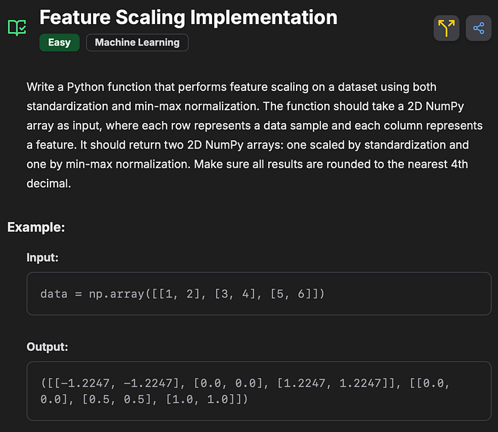
Problem Statement from Deep-ML —

import numpy as np
def feature_scaling(data: np.ndarray) -> (np.ndarray, np.ndarray):
 # Formula for both
 # normalized_data = (data - X_min) / (X_max - X_min)
 # standardized_data = (data - X_mean) / X_std

 X_min = np.min(data, axis=0)
 X_max = np.max(data, axis=0)

 X_mean = np.mean(data, axis=0)
 X_std = np.std(data, axis=0)
 
 normalized_data = (data - X_min) / (X_max - X_min)
 standardized_data = (data - X_mean) / (X_std)
 
 return standardized_data, normalized_data

The above code is the implementation for both Min-Max Scaling and Standard Scaling.

I also highly recommend checking the Learn section in the Deep-ML problem page whenever you’re getting stuck while solving the problem.

Confusion Matrix for Binary Classification

In ML, the confusion matrix is very confusing. But it still makes sense with practices. Let’s decode the concept step by step.

Before examining the confusion matrix, ensure you understand the classification problem in machine learning. In a classification setup, we get y_pred (a list of predicted values) after running our prediction model on X_test.

y_pred = [1,0,0,1,0] — Lets assume our y_pred looks like this. Now we already have a y_test from our split to test our prediction. y_test = [1,1,0,1,0]

y_pred = [1,0,0,1,0] and y_test = [1,1,0,1,0]

Now, to understand the accuracy of y_pred w.r.t. y_test, we use a confusion matrix.

You can read more about classification accuracy here. (Please continue after reading this article if you have no idea about classification accuracy.)

The accuracy of the above experiments is 4/5, as 4 out of 5 outcomes in y_pred are correct, corresponding to an 80% accuracy rate. But getting accuracy is not enough; a confusion matrix is created based on the outcomes to understand the results better. Here, the confusion matrix looks something like this —

Problem Statement from Deep-ML —

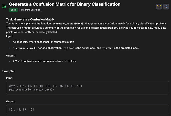
def confusion_matrix(data):
 # Implement the function here
 TP = 0 #True Positive
 FP = 0 #False Positive
 FN = 0 #False Negative
 TN = 0 #True Negative

 for y_test, y_pred in data:
 if y_test == 1 and y_pred == 1:
 TP += 1
 elif y_test == 1 and y_pred == 0:
 FN += 1
 elif y_test == 0 and y_pred == 1:
 FP += 1
 elif y_test == 0 and y_pred == 0:
 TN += 1
 return [[TP, FN],[FP, TN]]

These outputs (TN, FP, FN, TP) help to further calculate Precision, Recall, and F1 Score.

Overfitting & Underfitting

These two concepts mainly align with training and evaluating the Machine Learning models. Overfitting describes how well the model learned from the data so that it can generalize better to new data. On the other hand, Underfitting describes that the model was not able to learn properly from the training data.

Overfitting — High accuracy on training data, but lower accuracy on test data.

Underfitting — Low accuracy on both training and test data.

Problem Statement from Deep-ML —

Even though this problem is simple enough to solve, it clearly explains the concept.

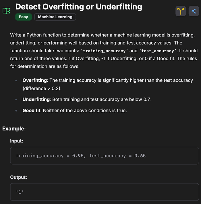
def model_fit_quality(training_accuracy, test_accuracy):
 """
 Determine if the model is overfitting, underfitting, or a good fit based on training and test accuracy.
 :param training_accuracy: float, training accuracy of the model (0 <= training_accuracy <= 1)
 :param test_accuracy: float, test accuracy of the model (0 <= test_accuracy <= 1)
 :return: int, one of '1', '-1', or '0'.
 """
 # Your code here
 if training_accuracy - test_accuracy > 0.2:
 return 1
 elif training_accuracy < 0.7 and test_accuracy < 0.7:
 return -1
 else:
 return 0

Random Shuffle of Dataset

This is a typically overlooked but very important concept to understand. When we discuss shuffling a dataset, it refers to shuffling the rows within it. This technique is useful because it helps reduce overfitting(by preventing bias). For example, we use this method when implementing the cross-validation technique.

Note: The shuffling technique can’t be used with time series data.

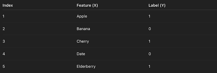
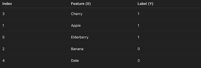
The above example is to explain the concept of shuffling visually.

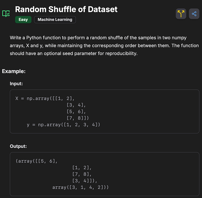
Problem Statement from Deep-ML —

import numpy as np

def shuffle_data(X, y, seed=None):
 np.random.seed(seed)
 indices = np.arange(len(X))
 np.random.shuffle(indices)
 return X[indices], y[indices]

If you examine the code above closely, we are also using np.random.seed to reproduce the results. This is important to pass the test cases.

Conclusion

These were only five examples I explained; you can visit Deep-ML to solve more such problems. And I highly encourage you to do so if you’re preparing for an AI/ML role. Please let me know in the comments section if you have enjoyed the article.

Thank you for reading. I love reading and writing content about AI and Machine Learning.

Join thousands of data leaders on the AI newsletter. Join over 80,000 subscribers and keep up to date with the latest developments in AI. From research to projects and ideas. If you are building an AI startup, an AI-related product, or a service, we invite you to consider becoming a sponsor.

Published via Towards AI