Why and How We t-Test

Author(s): Ayo Akinkugbe

Originally published on Towards AI.

Introduction

When running experiments — be it with models, prompts, or human evaluations — we often need to answer one deceptively simple question:

• Did the change or contribution we made with or research or experiment really make a difference?

or phrased differently — Are the differences we are seeing after experimenting our method actually meaningful, or just random noise?

This is what the t-test and other types of significance testing helps us answer.

What Significance Testing Does

Significance testing asks: If there were truly no real difference (often referred to as the null hypothesis), how likely is it that we’d observe results this extreme just by chance? If that likelihood — the p-value — is small (typically < 0.05), we say the result is statistically significant. In other words: our data suggest a real effect.

What does the p-value Really Mean?

The p-value is a measure of surprise under the assumption that nothing is going on. It answers the question: “If the null hypothesis were true — that there’s no real effect or difference — what’s the probability of getting results at least as extreme as the ones we observed, just by random chance?”

If the p-value is small (say, below 0.05), it means our observed difference would be very unlikely to occur if there were truly no effect. Therefore, we reject the null hypothesis and conclude that the difference is probably real. This threshold (0.05) is conventional, not magical — it corresponds to saying “I’m willing to accept a 5% chance that I’m wrong if I declare this effect real.”

So put plainly:

• p < 0.05 → Data is unlikely under “no effect” → evidence against the null hypothesis which rejects it → statistically significant.
• p > 0.05 → Data is not surprising under “no effect” → insufficient evidence → we fail to reject the null

The 0.05 threshold isn’t a mathematical rule. It traces back to the statistician Sir Ronald A. Fisher in the early 20th century (1920s–30s). Fisher proposed using p < 0.05 as a convenient standard for judging whether data provide substantial evidence against the null. It was never meant to be a hard cutoff — just a rule of thumb for balancing sensitivity (detecting real effects) and caution (avoiding false positives). But it caught on because it gave researchers a clear, consistent decision rule. Over time, journals and reviewers adopted it as a default — and it became institutionalized.

Common Misconceptions of the P-Value

• “p < 0.05 means the result is true.”

This is not true — it simply means the data are unlikely under the null, not that the alternative is guaranteed.

• “p > 0.05 means there’s no effect.”

Not necessarily — it might just mean we didn’t have enough data to detect significance.

• “p < 0.05 means the evidence favors the idea that a real effect exists.”

This is true. Though it doesn’t guarantee the results are true, it simply favors the notion that the results are significant

Common Types of Significance Tests

t-Test

The t-test is the classic tool for comparing two sample means and deciding whether their difference is large enough to be unlikely due to chance. It’s ideal when you have a numeric outcome and want to see if one group or condition performs differently from another — for instance, when comparing a new model against a baseline. At its core, the t-test measures how large the observed difference is relative to the variability in your data:

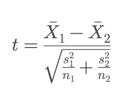
Here:

• Xs are the sample means
• Ss are the variances, and
• Ns are the sample sizes of each group.

This version (called Welch’s t-test) is the most common because it doesn’t assume equal variances. The formula expresses a simple idea:

t = (difference between means) / (standard error of that difference)

If the numerator (the difference) is large relative to the denominator (the noise), the resulting t-value will be large — and that makes it less likely that such a difference would appear by random chance under the “no effect” assumption.

Like all statistical tests, the t-test relies on some assumptions: that the data in each group are independent, approximately normal, and have reasonably similar variances. When these hold, the test tells you whether the observed gap in averages is statistically meaningful or just random noise.

Example for when to use: Did the new model produce higher average evaluation scores than the baseline?

ANOVA (Analysis of Variance)

The Analysis of Variance (ANOVA) extends the logic of the t-test to situations with three or more groups or conditions. Rather than running multiple t-tests (which would inflate the chance of false positives), ANOVA asks a single overarching question:

Are any of these group means significantly different from each other?

The idea is to compare how much the group means differ from the overall mean (the between-group variance) against how much variation there is within each group (the within-group variance). Mathematically, ANOVA uses the F-statistic:

Where:

• MS_between is the mean square due to differences among group means, and
• MS_within is the mean square due to random variation within groups.

If this ratio F is large — meaning the variation between groups is much greater than the natural variability within groups — ANOVA concludes that at least one group’s mean is significantly different. A key point is that ANOVA tells you that a difference exists, but not where it lies. When ANOVA finds a significant effect, you typically follow up with post-hoc tests (like Tukey’s HSD) to identify which specific groups differ.

Assumptions for ANOVA are similar to those for the t-test: observations should be independent, groups should be approximately normally distributed, and variances should be roughly equal.

Example for when to use: Do different model sizes (small, medium, large) perform differently on average?

Chi-square test

The Chi-square test applies when your data are categorical — that is, when you’re counting how many cases fall into different categories rather than measuring continuous values. It’s designed to test whether two categorical variables are independent or whether there’s a relationship between them.

The test compares what you actually observed with what you would expect to see if there were no association between the variables. The statistic is computed as:

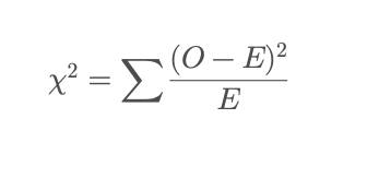
Where:

• O = observed count in each cell of the table
• E = expected count if the variables were independent

If the observed frequencies differ a lot from the expected ones, the Chi-square statistic becomes large — meaning that such a pattern of data would be unlikely to occur by random chance if the variables were truly unrelated.

Chi-square tests are especially useful for contingency tables (for example when comparing distributions of outcomes across groups) or checking whether observed proportions match theoretical ones. The test assumes that the data consist of independent observations and that expected frequencies aren’t too small (usually E is greater or equal to 5 per cell for reliable results).

Example for when to use: Are user ratings (positive, neutral, negative) distributed differently across model types?

Paired t-test / Wilcoxon signed-rank test

Whenever you collect two measurements from the same subjects — such as performance before and after an intervention or contribution — the samples are paired, not independent. In these situations, the Paired t-test evaluates whether the average difference between the two sets of measurements is significantly different from zero.

Instead of comparing two separate group means, it looks at differences within each pair, treating each subject as their own control. The formula is:

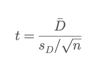
Where:

• D = mean of the differences between paired values
• s_D = standard deviation of those differences
• n = number of pairs

This approach accounts for the natural correlation between repeated measures on the same entity, making the test more sensitive to detecting real effects than an independent-samples t-test. The main assumption is that these differences (D_i) are approximately normally distributed.

If that assumption doesn’t hold — for example, if the data are skewed or contain outliers — the Wilcoxon signed-rank test provides a nonparametric alternative. Instead of working with the raw differences, it ranks them by magnitude (ignoring sign), then checks whether positive and negative ranks are balanced around zero. This makes it more robust to non-normal data while testing the same core question:

Are the paired measurements systematically higher or lower after the change?

Example for when to use: Did participants’ accuracy improve after receiving feedback?

Mann–Whitney U test

The Mann–Whitney U test (also known as the Wilcoxon rank-sum test) is a nonparametric alternative to the independent-samples t-test. It’s ideal when your data don’t meet the normality assumption or when your measurements are ordinal — for instance, rankings, ratings, or other ordered categories.

Rather than comparing means, the Mann–Whitney U test compares the distributions of two groups — asking whether values in one group tend to be larger or smaller than those in the other. It does this by ranking all the observations from both groups together, then summing the ranks for each group.

The test statistic is calculated as:

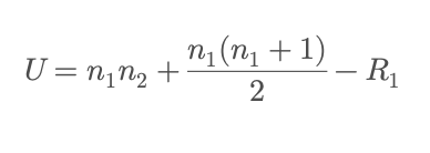
Where:

• ns are the sample sizes of the two groups, and
• R_1 is the sum of ranks for group 1.

A smaller U value means that the ranks from one group are generally lower (or higher) than the other — indicating a systematic difference between the two distributions. Because the test uses ranks rather than raw values, it’s robust to outliers and skewed data, making it a great choice when data don’t follow a normal distribution or include extreme values.

While it’s often interpreted as comparing medians, technically the Mann–Whitney U test assesses whether one distribution tends to produce larger values than the other — a subtle but important distinction.

Example: Are median rewards higher for one reinforcement learning policy than another?

Correlation tests (Pearson, Spearman)

Correlation tests measure the strength and direction of association between two variables — in other words, how closely changes in one variable are related to changes in another.

The Pearson correlation coefficient is the most common measure of linear relationship between two continuous, normally distributed variables. It answers the question:

“As X increases, does Y tend to increase (or decrease) in a roughly straight-line pattern?”

The formula for Pearson’s r is:

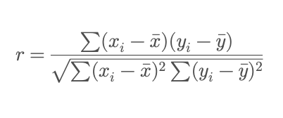
Where:

• x_i, y_i are paired observations,
• x and y bare are their means.

The value of r ranges from –1 to +1:

• +1: perfect positive linear relationship
• 0: no linear relationship
• –1: perfect negative linear relationship

If your data are not normally distributed, contain outliers, or are ordinal (ranked but not evenly spaced), the Spearman rank correlation is a better choice. It computes Pearson’s correlation on the ranks of the data instead of the raw values, capturing any monotonic relationship — one where variables move in the same general direction, even if not linearly.

Both correlations can be tested for statistical significance, helping you judge whether an observed relationship is likely real or could have arisen by chance.

Example: Does prompt length correlate with output quality or evaluation consistency?

Regression significance tests

Regression analysis goes beyond simple comparisons by modeling how one or more predictor variables influence a continuous outcome. Each predictor (or coefficient) in a regression model represents an estimated relationship — for example, how much a change in one variable is associated with a change in the outcome, holding others constant.

To determine whether a predictor’s effect is statistically meaningful or just noise, regression uses significance tests on coefficients, typically with the t-statistic:

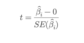
Where:

• Beta is the estimated coefficient for predictor i, and
• SE(Beta) is its standard error.

This test checks whether the coefficient is significantly different from zero — in other words, whether that predictor has a real effect on the outcome after accounting for variability. Regression models can also be assessed as a whole using the F-test, which compares the model’s explained variance to the unexplained variance:

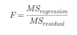
A large F-statistic indicates that the model explains a meaningful portion of the total variability in the outcome compared to random noise. These tests help answer both levels of questions:

• Which predictors truly matter? (via t-tests)
• Does the model overall explain the data better than chance? (via F-test)

Regression significance tests assume that residuals are independent, normally distributed, and have constant variance (homoscedasticity). When those conditions hold, they provide a rigorous way to evaluate both individual effects and overall model fit.

Example: Does model size significantly predict performance accuracy after controlling for training data size?

Choosing the Right Test

Though there are various types of significance tests, here are some questions that might point you towards choosing the right one for your research experiment:

1. How many groups or conditions am I comparing?
2. Are my samples independent or paired?
3. Is my data roughly normal, or skewed/nonparametric?
4. Am I comparing averages, proportions, or relationships?

Your answers should guide you to the right test:

• Two groups, numeric data → t-test
• More than two → ANOVA
• Categorical counts → Chi-square
• Non-normal or ordinal data → Mann–Whitney / Wilcoxon
• Relationships → Correlation or regression tests

How We t-Test (or Test for Significance)

Performing a t-test is a structured process. Here’s a step-by-step approach:

Step 1 — Form hypotheses

Every t-test begins with a clear question, expressed as hypotheses or assumptions or educated guesses:

• Null hypothesis (H₀): In this assumption there’s no real difference between the groups; any observed difference is due to chance.
• Alternative hypothesis (H₁): Here, the new condition or treatment performs differently than the baseline.

Formulating hypotheses ensures you know exactly what you’re testing before seeing the data, preventing “fishing” for significance.

Step 2— Compute

Next, calculate the summary statistics for each group: the mean and variance. Then compute the t-statistic:

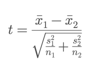
This formula measures the difference between means relative to the combined variability of the groups. A larger t-value indicates a larger difference relative to the noise.

Finally, compare the t-value to a reference distribution (the t-distribution) to find the p-value. Modern software and libraries (e.g scipy.stats) handles this automatically, but the logic is the same: determine whether the observed difference is unlikely under the null.

Step 3— Interpret

• Small p-value (e.g < 0.05): The difference is unlikely to be due to chance — the result is statistically significant.
• Large p-value: The observed difference could plausibly occur under the null — we cannot conclude a real effect.

Remember: a significant result does not automatically imply a meaningful or large effect — always complement with effect sizes and confidence intervals (See under Going Beyond the p-Value).

Step 4— Check assumptions

The validity of the t-test depends on a few key assumptions:

1. Rough normality: Each group’s data should be approximately normally distributed.
2. Independent samples: Observations in one group shouldn’t influence those in the other.
3. Similar variances: Groups should have roughly equal variance. If not, use Welch’s t-test, which adjusts for unequal variances.

Checking these assumptions ensures that your p-values and conclusions are reliable.

Going Beyond the p-Value

The t-test tells us if the difference is significant — not how large or how meaningful it is. That’s why we always complement it with the following:

Effect size (e.g., Cohen’s d)

While the p-value answers “Is there a difference?”, the effect size answers- “How big is that difference?”

For a t-test, a common measure is Cohen’s d:

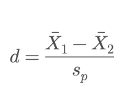
where s_p is the pooled standard deviation. Roughly speaking,

• 0.2 = small effect
• 0.5 = medium
• 0.8 = large

Reporting effect size helps translate statistical results into real-world meaning, showing whether an effect is trivial or substantial.

Confidence intervals

A confidence interval gives a range of plausible values for the true effect in the population. For example, a 95% confidence interval for a mean difference might run from 0.3 to 1.2, suggesting we’re fairly confident the real effect lies somewhere in that range. Narrow intervals indicate precision, while wide ones reveal uncertainty. Unlike the binary “significant / not significant” label of a p-value, confidence intervals show both magnitude and reliability.

The general formular for finding the confidence interval is:

Where:

• Estimate = the sample statistic you’re interested in (e.g., a sample mean or the difference between two sample means).
• Standard Error (SE) = how much that estimate would vary if you repeated the experiment many times.
• t* = the critical value from the t-distribution, based on your chosen confidence level (like 95%) and your degrees of freedom.

Visual inspection of distributions

Finally, it’s good practice to plot your data — using boxplots, histograms, or violin plots. Visualizations often reveal overlap, skew, or outliers that a single test statistic can obscure. Two groups may differ significantly, yet still overlap heavily in their distributions — a reminder that statistical and practical meaning can diverge.

Together, these additional approaches give a more complete picture:

• the p-value says “something’s likely happening”
• the effect size says “how much it matters”, and
• the confidence interval and visualization show “how sure we are and what the plausible range of the true effect looks like”

Conclusion

We t-test — and, more broadly, perform significance testing — not because statistics demand it, but because our experiments deserve rigorous evaluation. These tests help us reason clearly, communicate results responsibly, and distinguish signal from noise.

But significance alone isn’t enough. Complementing p-values with effect sizes, confidence intervals, and visualizations ensures we understand not just whether an effect exists, but how large it is, how reliable it is, and what it really looks like.

In the end, testing for significance is a tool for better decision-making, not just number-crunching. It allows us to report findings transparently, interpret them thoughtfully, and build knowledge that others can trust and build upon.

For more on AI Research 🧪, Check out other posts in this series:

Ayo Akinkugbe

AI Research

View list1 story

Join thousands of data leaders on the AI newsletter. Join over 80,000 subscribers and keep up to date with the latest developments in AI. From research to projects and ideas. If you are building an AI startup, an AI-related product, or a service, we invite you to consider becoming a sponsor.

Published via Towards AI