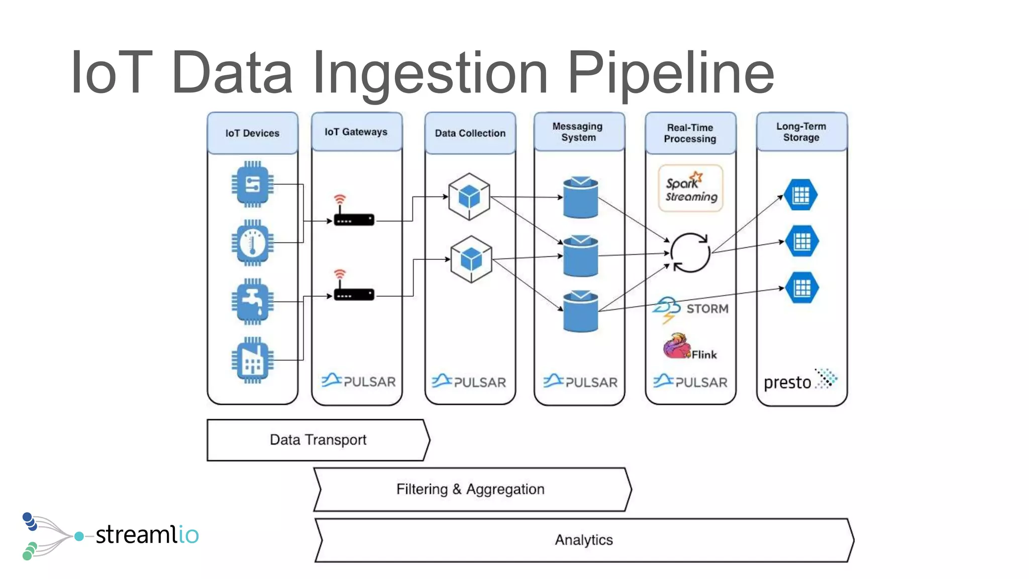
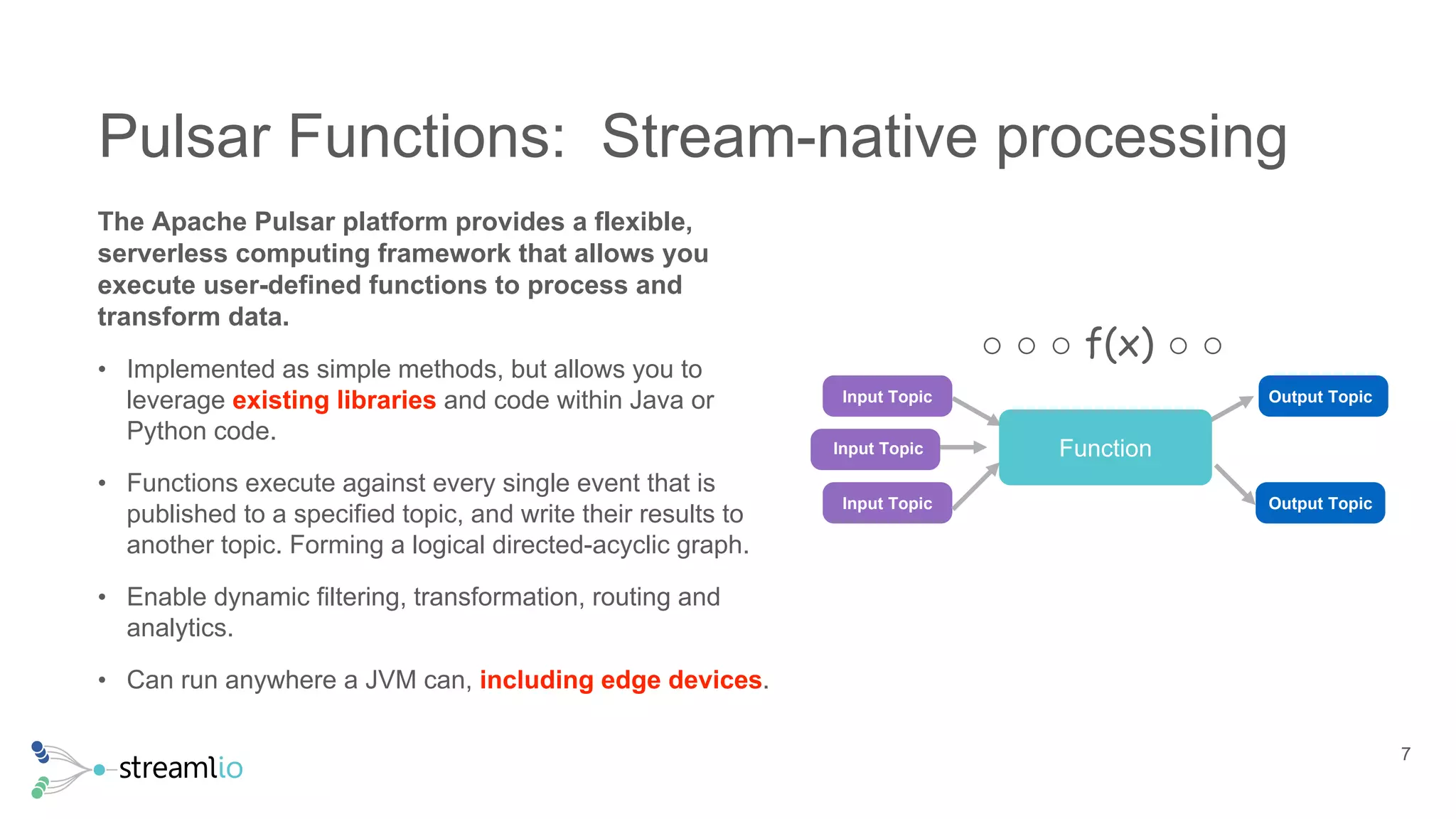
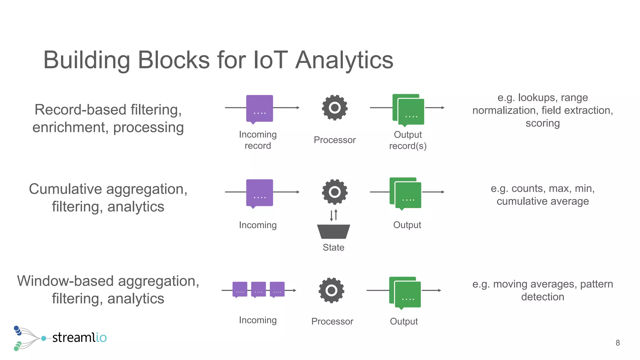
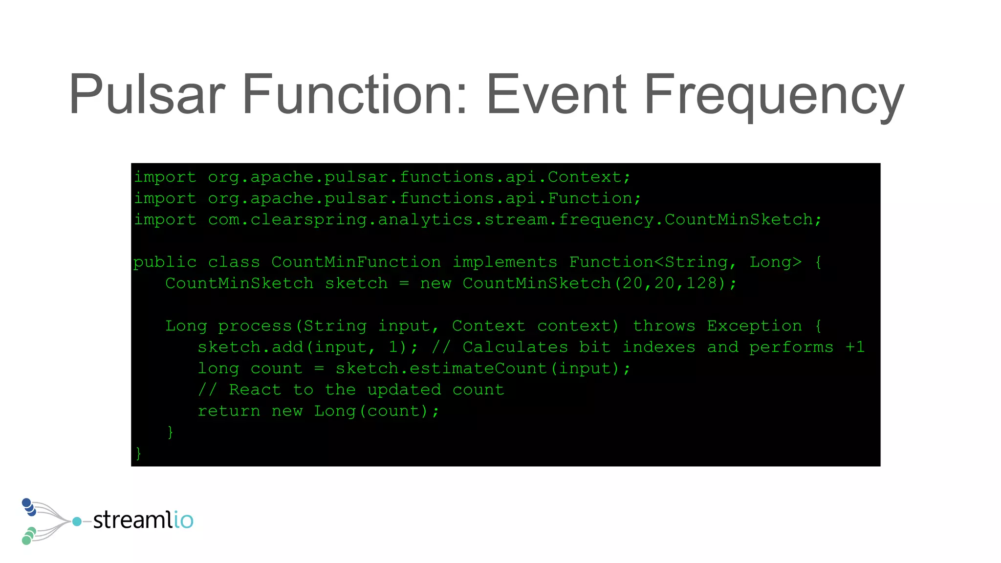
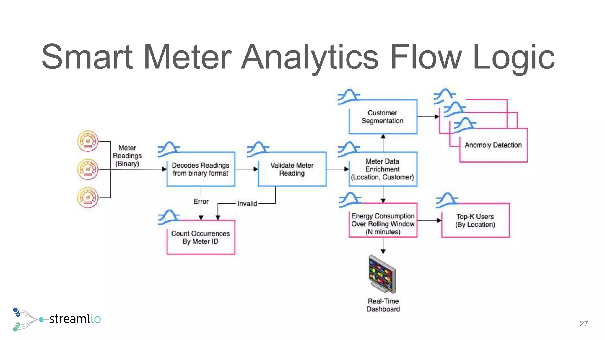
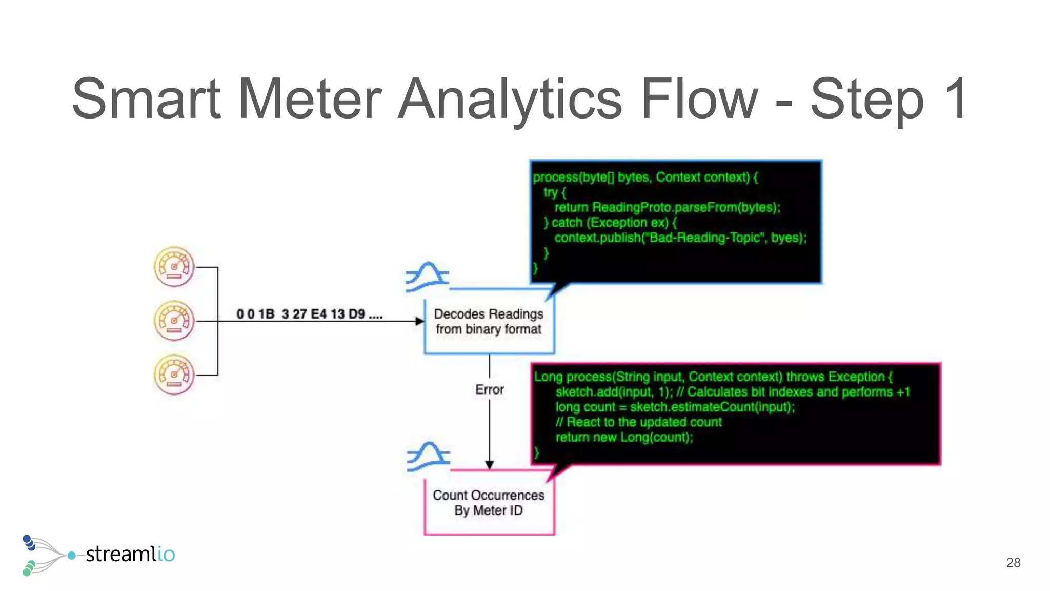
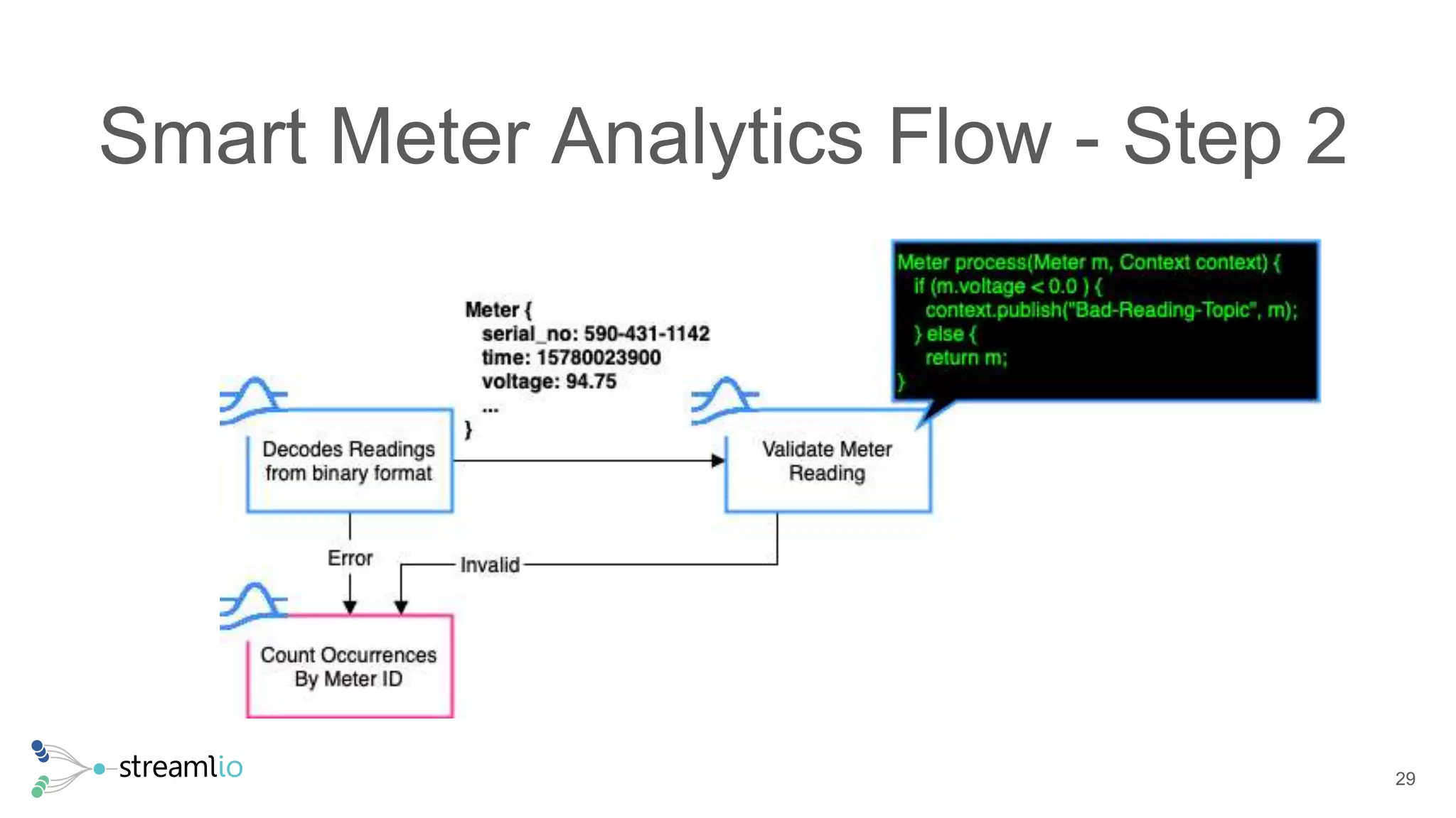
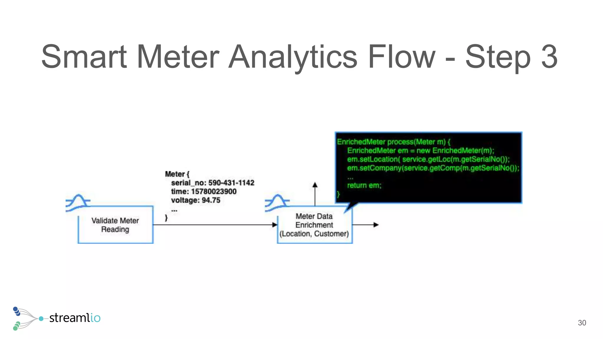
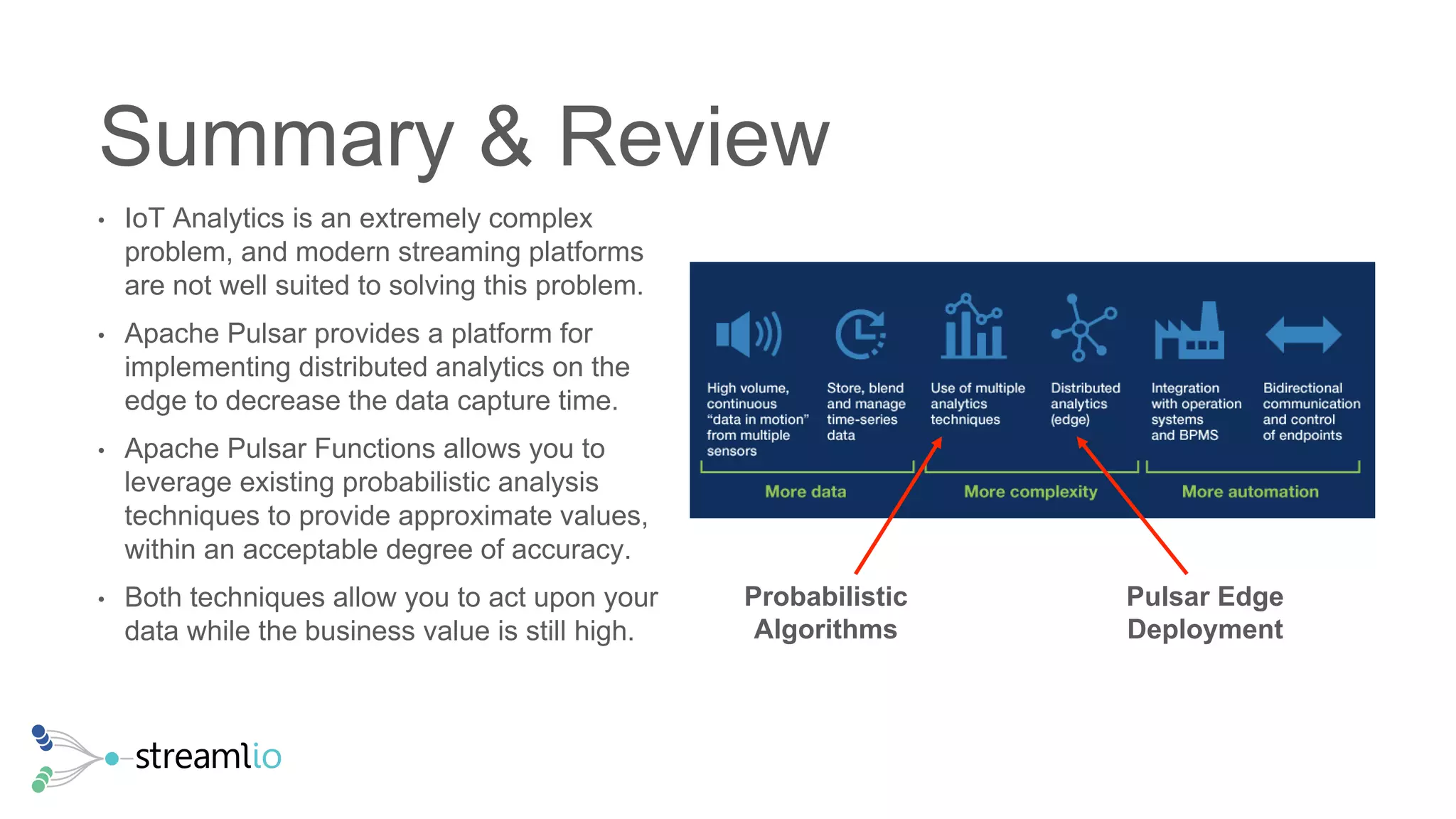
Real-Time IoT Analytics with Apache Pulsar May 22nd, 2019 David Kjerrumgaard
• It is NOT JUST loading sensor data into a data lake to create predictive analytic models. While this is crucial piece of the puzzle, it is not the only one. • IoT Analytics requires the ability to ingest, aggregate, and process an endless stream of real-time data coming off a wide variety of sensor devices “at the edge” • IoT Analytics renders real-time decisions at the edge of the network to either optimize operational performance or detect anomalies for immediate remediation. Defining IoT Analytics
What Makes IoT Analytics Different?
• IoT deals with machine generated data consisting of discrete observations such as temperature, vibration, pressure, etc. that is produced at very high rates. • We need an architecture that: • Allows us to quickly identify and react to anomalous events • Reduces the volume of data transmitted back to the data lake. • In this talk, we will present a solution based on Apache Pulsar Functions that distributes the analytics processing across all tiers of the IoT data ingestion pipeline. IoT Analytics Challenges
IoT Data Ingestion Pipeline
Apache Pulsar Functions
The Apache Pulsar platform provides a flexible, serverless computing framework that allows you execute user-defined functions to process and transform data. • Implemented as simple methods, but allows you to leverage existing libraries and code within Java or Python code. • Functions execute against every single event that is published to a specified topic, and write their results to another topic. Forming a logical directed-acyclic graph. • Enable dynamic filtering, transformation, routing and analytics. • Can run anywhere a JVM can, including edge devices. Pulsar Functions: Stream-native processing 7 Input Topic Function f(x) Input Topic Input Topic Output Topic Output Topic
Building Blocks for IoT Analytics 8 Record-based filtering, enrichment, processing Incoming record …. Processor …. Output record(s) e.g. lookups, range normalization, field extraction, scoring …. Cumulative aggregation, filtering, analytics e.g. counts, max, min, cumulative average Incoming …. Output State ….…. Window-based aggregation, filtering, analytics e.g. moving averages, pattern detection Incoming …. Processor …. Output …. …. ….
Distributed Probabilistic Analytics with Apache Pulsar Functions
Probabilistic Analysis • Often times, it is sufficient to provide an approximate value when it is impossible and/or impractical to provide a precise value. In many cases having an approximate answer within a given time frame is better than waiting for an exact answer. • Probabilistic algorithms can provide approximate values when the event stream is either too large to store in memory, or the data is moving too fast to process. • Instead of requiring to keep such enormous data on-hand, we leverage algorithms that require only a few kilobytes of data.
Data Sketches • A central theme throughout most of these probabilistic data structures is the concept of data sketches, which are designed to require only enough of the data necessary to make an accurate estimation of the correct answer. • Typically, sketches are implemented a bit arrays or maps thereby requiring memory on the order of Kilobytes, making them ideal for resource-constrained environments, e.g. on the edge. • Sketching algorithms only need to see each incoming item only once, and are therefore ideal for processing infinite streams of data.
• Let’s walk through an demonstration to show exactly what I mean by sketches and show you that we do not need 100% of the data in order to make an accurate prediction of what the picture contains • How much of the data did you require to identify the main item in the picture? Sketch Example
Data Sketch Properties • Configurable Accuracy • Sketches sized correctly can be 100% accurate • Error rate is inversely proportional to size of a Sketch • Fixed Memory Utilization • Maximum Sketch size is configured in advance • Memory cost of a query is thus known in advance • Allows Non-additive Operations to be Additive • Sketches can be merged into a single Sketch without over counting • Allows tasks to be parallelized and combined later • Allows results to be combined across windows of execution
Operations Supported by Sketches Theta Sketch Count Distinct Example: when you're doing profiling at the router level, you often want to estimate functions of distinct IP addresses, and since you can't just maintain counters for each possible address. Theta Sketches enable us to answer questions about the number of unique users (set union), the number of users who did X and Y (set intersection), and the number of users who did X and did not do Y (set disjunction). Tuple Sketch Group By Tuple Sketches are ideal for summarizing attributes such as impressions or clicks. Tuple Sketches also provide sufficient methods so that user could develop a wrapper class that could facilitate approximate joins or other common database operations. Quantile Sketches Distribution Anomaly Detection Consider this real data example of a stream of 230 million time-spent events collected from one our systems for a period of just 30 minutes. Each event records the amount of time in milliseconds that a user spends on a web page before moving to a different web page by taking some action, such as a click. Calculate the distribution of this dataset, then determine for a given value where it lies within the distribution. Anything with the 99th percentile would be considered anomalous and flagged for action. Frequent Items Sketches Top-K Frequency estimation of Internet packet streams. Top-10 Tweets, Queries, items sold, etc. Sampling Approximate Query Processing What is the ratio of ? What percentage of ? What is the average of ? Approximate query processing is a viable technique to use in these cases. A slightly less accurate result but which is computed instantly is desirable in these cases. This is because most analysts are performing exploratory operation on the database and do not need precise answers. An approximate answer along with a confidence interval would suit most of the use cases.
Some Sketchy Functions
• Another common statistic computed is the frequency at which a specific element occurs within an endless data stream with repeated elements, which enables us to answer questions such as; “How many times has element X occurred in the data stream?”. • Consider trying to analyze and sample the IoT sensor data for just a single industrial plant that can produce millions of readings per second. There isn’t enough time to perform the calculations or store the data. • In such a scenario you can chose to forego an exact answer, which will we never be able to compute in time, for an approximate answer that is within an acceptable range of accuracy. Event Frequency
• The Count-Min Sketch algorithm uses two elements: • An M-by-K matrix of counters, each initialized to 0, where each row corresponds to a hash function • A collection of K independent hash functions h(x). • When an element is added to the sketch, each of the hash functions are applied to the element. These hash values are treated as indexes into the bit array, and the corresponding array element is set incremented by 1. • Now that we have an approximate count for each element we have seen stored in the M-by-K matrix, we are able to quickly determine how many times an element X has occurred previously in the stream by simply applying each of the hash functions to the element, and retrieving all of the corresponding array elements and using the SMALLEST value in the list are the approximate event count. Count-Min Sketch
Pulsar Function: Event Frequency import org.apache.pulsar.functions.api.Context; import org.apache.pulsar.functions.api.Function; import com.clearspring.analytics.stream.frequency.CountMinSketch; public class CountMinFunction implements Function<String, Long> { CountMinSketch sketch = new CountMinSketch(20,20,128); Long process(String input, Context context) throws Exception { sketch.add(input, 1); // Calculates bit indexes and performs +1 long count = sketch.estimateCount(input); // React to the updated count return new Long(count); } }
• Another common use of the Count-Min algorithm is maintaining lists of frequent items which is commonly referred to as the “Heavy Hitters”. This design pattern retains a list of items that occur more frequently than some predefined value, e.g. the top-K list • The K-Frequency-Estimation problem can also be solved by using the Count-Min Sketch algorithm. The logic for updating the counts is exactly the same as in the Event Frequency use case. • However, there is an additional list of length K used to keep the top-K elements seen that is updated. K-Frequency-Estimation, aka “Heavy Hitters”
Pulsar Function: Top K • Each of the hash functions are applied to the element. These hash values are treated as indexes into the bit array, and the corresponding array element is set incremented by 1. • Calculate the event frequency for the element as we did in the event frequency use case. However, this time we take the SMALLEST value in the list are use that as the approximate event count. • Compare the calculated event frequency of this element against the smallest value in the top-K elements array, and if it is LARGER, remove the smallest value and replace it with the new element.
Pulsar Function: Top K import org.apache.pulsar.functions.api.Context; import org.apache.pulsar.functions.api.Function; import com.clearspring.analytics.stream.StreamSummary; public class CountMinFunction implements Function<String, List<Counter<String>>> { StreamSummary<String> summary = new StreamSummary<String> (256); List<Counter<String>> process(String input, Context context) throws Exception { // Add the element to the sketch summary.offer(input, 1) // Grab the updated top 10 List<Counter<String>> topK = summary.topK(10); return topK; } }
• The most anomaly detectors use a manually configured threshold value that is not adaptive to even simple patterns or variances. • Instead of using a single static value for our thresholds, we should consider using quantiles instead. • In statistics and probably, quantiles are used to represent probability distributions. The most common of which are known as percentiles. Anomaly Detection
• The data structure known as t-digest was developed by Ted Dunning, as a way to accurately estimate extreme quantiles for very large data sets with limited memory use. • This capability makes t-digest particularly useful for calculating quantiles that can be used to select a good threshold for anomaly detection. • The advantage of this approach is that the threshold automatically adapts to the dataset as it collects more data. Anomaly Detection with Quantiles
Pulsar Function: T-Digest import com.clearspring.analytics.stream.quantile.TDigest; public AnomalyDetectorFunction implements Function<Sensor s, Void> { private static TDigest digest; Void process(Sensor s, Context context) throws Exception { Double threshold = context.getUserConfigValue(“threshold”).toString(); String alertTopic = context.getUserConfigValue(“alert-topic”).toString(); getDigest().add(s.getMetric()); // Add metric to observations Double quantile = getDigest().compute(s.getMetric()); if (quantile > threshold) { context.publish(alertTopic, sensor.getId()); } return null; } private static TDigest getDigest() { if (digest == null) { digest = new TDigest(100); // Accuracy = 3/100 = 3% } return digest; } }
IoT Analytics Pipeline Using Apache Pulsar Functions
• A network of smart meters enables utilities companies to gain greater visibility into their customers energy consumption. • Increase/decrease energy generation to meet the demand • Implement dynamic notifications to encourage consumers to use less energy during peak demand periods. • Provide real-time revenue forecasts to senior business leaders. • Identify fault meters and schedule maintenance calls to repair them. Identifying Real-Time Energy Consumption Patterns
Smart Meter Analytics Flow Logic 27
Smart Meter Analytics Flow - Step 1 28
Smart Meter Analytics Flow - Step 2 29
Smart Meter Analytics Flow - Step 3 30
Smart Meter Analytics Flow - Step 4 31
Smart Meter Analytics Flow - Step 5 32
Smart Meter Analytics Flow - Step 6 33
Summary & Review
• IoT Analytics is an extremely complex problem, and modern streaming platforms are not well suited to solving this problem. • Apache Pulsar provides a platform for implementing distributed analytics on the edge to decrease the data capture time. • Apache Pulsar Functions allows you to leverage existing probabilistic analysis techniques to provide approximate values, within an acceptable degree of accuracy. • Both techniques allow you to act upon your data while the business value is still high. Summary & Review Probabilistic Algorithms Pulsar Edge Deployment
Questions
Thank You!!

Using Apache Pulsar to Provide Real-Time IoT Analytics on the Edge

  • 1.
    Real-Time IoT Analytics withApache Pulsar May 22nd, 2019 David Kjerrumgaard
  • 2.
    • It isNOT JUST loading sensor data into a data lake to create predictive analytic models. While this is crucial piece of the puzzle, it is not the only one. • IoT Analytics requires the ability to ingest, aggregate, and process an endless stream of real-time data coming off a wide variety of sensor devices “at the edge” • IoT Analytics renders real-time decisions at the edge of the network to either optimize operational performance or detect anomalies for immediate remediation. Defining IoT Analytics
  • 3.
    What Makes IoTAnalytics Different?
  • 4.
    • IoT dealswith machine generated data consisting of discrete observations such as temperature, vibration, pressure, etc. that is produced at very high rates. • We need an architecture that: • Allows us to quickly identify and react to anomalous events • Reduces the volume of data transmitted back to the data lake. • In this talk, we will present a solution based on Apache Pulsar Functions that distributes the analytics processing across all tiers of the IoT data ingestion pipeline. IoT Analytics Challenges
  • 5.
  • 6.
  • 7.
    The Apache Pulsarplatform provides a flexible, serverless computing framework that allows you execute user-defined functions to process and transform data. • Implemented as simple methods, but allows you to leverage existing libraries and code within Java or Python code. • Functions execute against every single event that is published to a specified topic, and write their results to another topic. Forming a logical directed-acyclic graph. • Enable dynamic filtering, transformation, routing and analytics. • Can run anywhere a JVM can, including edge devices. Pulsar Functions: Stream-native processing 7 Input Topic Function f(x) Input Topic Input Topic Output Topic Output Topic
  • 8.
    Building Blocks forIoT Analytics 8 Record-based filtering, enrichment, processing Incoming record …. Processor …. Output record(s) e.g. lookups, range normalization, field extraction, scoring …. Cumulative aggregation, filtering, analytics e.g. counts, max, min, cumulative average Incoming …. Output State ….…. Window-based aggregation, filtering, analytics e.g. moving averages, pattern detection Incoming …. Processor …. Output …. …. ….
  • 9.
  • 10.
    Probabilistic Analysis • Oftentimes, it is sufficient to provide an approximate value when it is impossible and/or impractical to provide a precise value. In many cases having an approximate answer within a given time frame is better than waiting for an exact answer. • Probabilistic algorithms can provide approximate values when the event stream is either too large to store in memory, or the data is moving too fast to process. • Instead of requiring to keep such enormous data on-hand, we leverage algorithms that require only a few kilobytes of data.
  • 11.
    Data Sketches • Acentral theme throughout most of these probabilistic data structures is the concept of data sketches, which are designed to require only enough of the data necessary to make an accurate estimation of the correct answer. • Typically, sketches are implemented a bit arrays or maps thereby requiring memory on the order of Kilobytes, making them ideal for resource-constrained environments, e.g. on the edge. • Sketching algorithms only need to see each incoming item only once, and are therefore ideal for processing infinite streams of data.
  • 12.
    • Let’s walkthrough an demonstration to show exactly what I mean by sketches and show you that we do not need 100% of the data in order to make an accurate prediction of what the picture contains • How much of the data did you require to identify the main item in the picture? Sketch Example
  • 13.
    Data Sketch Properties •Configurable Accuracy • Sketches sized correctly can be 100% accurate • Error rate is inversely proportional to size of a Sketch • Fixed Memory Utilization • Maximum Sketch size is configured in advance • Memory cost of a query is thus known in advance • Allows Non-additive Operations to be Additive • Sketches can be merged into a single Sketch without over counting • Allows tasks to be parallelized and combined later • Allows results to be combined across windows of execution
  • 14.
    Operations Supported bySketches Theta Sketch Count Distinct Example: when you're doing profiling at the router level, you often want to estimate functions of distinct IP addresses, and since you can't just maintain counters for each possible address. Theta Sketches enable us to answer questions about the number of unique users (set union), the number of users who did X and Y (set intersection), and the number of users who did X and did not do Y (set disjunction). Tuple Sketch Group By Tuple Sketches are ideal for summarizing attributes such as impressions or clicks. Tuple Sketches also provide sufficient methods so that user could develop a wrapper class that could facilitate approximate joins or other common database operations. Quantile Sketches Distribution Anomaly Detection Consider this real data example of a stream of 230 million time-spent events collected from one our systems for a period of just 30 minutes. Each event records the amount of time in milliseconds that a user spends on a web page before moving to a different web page by taking some action, such as a click. Calculate the distribution of this dataset, then determine for a given value where it lies within the distribution. Anything with the 99th percentile would be considered anomalous and flagged for action. Frequent Items Sketches Top-K Frequency estimation of Internet packet streams. Top-10 Tweets, Queries, items sold, etc. Sampling Approximate Query Processing What is the ratio of ? What percentage of ? What is the average of ? Approximate query processing is a viable technique to use in these cases. A slightly less accurate result but which is computed instantly is desirable in these cases. This is because most analysts are performing exploratory operation on the database and do not need precise answers. An approximate answer along with a confidence interval would suit most of the use cases.
  • 15.
  • 16.
    • Another commonstatistic computed is the frequency at which a specific element occurs within an endless data stream with repeated elements, which enables us to answer questions such as; “How many times has element X occurred in the data stream?”. • Consider trying to analyze and sample the IoT sensor data for just a single industrial plant that can produce millions of readings per second. There isn’t enough time to perform the calculations or store the data. • In such a scenario you can chose to forego an exact answer, which will we never be able to compute in time, for an approximate answer that is within an acceptable range of accuracy. Event Frequency
  • 17.
    • The Count-MinSketch algorithm uses two elements: • An M-by-K matrix of counters, each initialized to 0, where each row corresponds to a hash function • A collection of K independent hash functions h(x). • When an element is added to the sketch, each of the hash functions are applied to the element. These hash values are treated as indexes into the bit array, and the corresponding array element is set incremented by 1. • Now that we have an approximate count for each element we have seen stored in the M-by-K matrix, we are able to quickly determine how many times an element X has occurred previously in the stream by simply applying each of the hash functions to the element, and retrieving all of the corresponding array elements and using the SMALLEST value in the list are the approximate event count. Count-Min Sketch
  • 18.
    Pulsar Function: EventFrequency import org.apache.pulsar.functions.api.Context; import org.apache.pulsar.functions.api.Function; import com.clearspring.analytics.stream.frequency.CountMinSketch; public class CountMinFunction implements Function<String, Long> { CountMinSketch sketch = new CountMinSketch(20,20,128); Long process(String input, Context context) throws Exception { sketch.add(input, 1); // Calculates bit indexes and performs +1 long count = sketch.estimateCount(input); // React to the updated count return new Long(count); } }
  • 19.
    • Another commonuse of the Count-Min algorithm is maintaining lists of frequent items which is commonly referred to as the “Heavy Hitters”. This design pattern retains a list of items that occur more frequently than some predefined value, e.g. the top-K list • The K-Frequency-Estimation problem can also be solved by using the Count-Min Sketch algorithm. The logic for updating the counts is exactly the same as in the Event Frequency use case. • However, there is an additional list of length K used to keep the top-K elements seen that is updated. K-Frequency-Estimation, aka “Heavy Hitters”
  • 20.
    Pulsar Function: TopK • Each of the hash functions are applied to the element. These hash values are treated as indexes into the bit array, and the corresponding array element is set incremented by 1. • Calculate the event frequency for the element as we did in the event frequency use case. However, this time we take the SMALLEST value in the list are use that as the approximate event count. • Compare the calculated event frequency of this element against the smallest value in the top-K elements array, and if it is LARGER, remove the smallest value and replace it with the new element.
  • 21.
    Pulsar Function: TopK import org.apache.pulsar.functions.api.Context; import org.apache.pulsar.functions.api.Function; import com.clearspring.analytics.stream.StreamSummary; public class CountMinFunction implements Function<String, List<Counter<String>>> { StreamSummary<String> summary = new StreamSummary<String> (256); List<Counter<String>> process(String input, Context context) throws Exception { // Add the element to the sketch summary.offer(input, 1) // Grab the updated top 10 List<Counter<String>> topK = summary.topK(10); return topK; } }
  • 22.
    • The mostanomaly detectors use a manually configured threshold value that is not adaptive to even simple patterns or variances. • Instead of using a single static value for our thresholds, we should consider using quantiles instead. • In statistics and probably, quantiles are used to represent probability distributions. The most common of which are known as percentiles. Anomaly Detection
  • 23.
    • The datastructure known as t-digest was developed by Ted Dunning, as a way to accurately estimate extreme quantiles for very large data sets with limited memory use. • This capability makes t-digest particularly useful for calculating quantiles that can be used to select a good threshold for anomaly detection. • The advantage of this approach is that the threshold automatically adapts to the dataset as it collects more data. Anomaly Detection with Quantiles
  • 24.
    Pulsar Function: T-Digest importcom.clearspring.analytics.stream.quantile.TDigest; public AnomalyDetectorFunction implements Function<Sensor s, Void> { private static TDigest digest; Void process(Sensor s, Context context) throws Exception { Double threshold = context.getUserConfigValue(“threshold”).toString(); String alertTopic = context.getUserConfigValue(“alert-topic”).toString(); getDigest().add(s.getMetric()); // Add metric to observations Double quantile = getDigest().compute(s.getMetric()); if (quantile > threshold) { context.publish(alertTopic, sensor.getId()); } return null; } private static TDigest getDigest() { if (digest == null) { digest = new TDigest(100); // Accuracy = 3/100 = 3% } return digest; } }
  • 25.
    IoT Analytics PipelineUsing Apache Pulsar Functions
  • 26.
    • A networkof smart meters enables utilities companies to gain greater visibility into their customers energy consumption. • Increase/decrease energy generation to meet the demand • Implement dynamic notifications to encourage consumers to use less energy during peak demand periods. • Provide real-time revenue forecasts to senior business leaders. • Identify fault meters and schedule maintenance calls to repair them. Identifying Real-Time Energy Consumption Patterns
  • 27.
    Smart Meter AnalyticsFlow Logic 27
  • 28.
    Smart Meter AnalyticsFlow - Step 1 28
  • 29.
    Smart Meter AnalyticsFlow - Step 2 29
  • 30.
    Smart Meter AnalyticsFlow - Step 3 30
  • 31.
    Smart Meter AnalyticsFlow - Step 4 31
  • 32.
    Smart Meter AnalyticsFlow - Step 5 32
  • 33.
    Smart Meter AnalyticsFlow - Step 6 33
  • 34.
  • 35.
    • IoT Analyticsis an extremely complex problem, and modern streaming platforms are not well suited to solving this problem. • Apache Pulsar provides a platform for implementing distributed analytics on the edge to decrease the data capture time. • Apache Pulsar Functions allows you to leverage existing probabilistic analysis techniques to provide approximate values, within an acceptable degree of accuracy. • Both techniques allow you to act upon your data while the business value is still high. Summary & Review Probabilistic Algorithms Pulsar Edge Deployment
  • 36.
  • 37.

Editor's Notes

  • #28 Incomplete--morph David’s EDA example to a (very) simple data pipeline
  • #29 Incomplete--morph David’s EDA example to a (very) simple data pipeline
  • #30 Incomplete--morph David’s EDA example to a (very) simple data pipeline
  • #31 Incomplete--morph David’s EDA example to a (very) simple data pipeline
  • #32 Incomplete--morph David’s EDA example to a (very) simple data pipeline
  • #33 Incomplete--morph David’s EDA example to a (very) simple data pipeline
  • #34 Incomplete--morph David’s EDA example to a (very) simple data pipeline