Unit I- Data structures Introduction, Evaluation of Algorithms, Arrays, Sparse Matrix
The document provides a comprehensive syllabus on data structures and algorithms, covering topics such as arrays, linked lists, trees, graphs, sorting methods, and performance evaluation techniques. It emphasizes the significance of data structures in organizing and managing data effectively, as well as algorithm analysis in terms of time and space complexity. Additionally, it includes practical examples, assignments, and feedback mechanisms for enhanced learning and understanding.
Unit I- Data structures Introduction, Evaluation of Algorithms, Arrays, Sparse Matrix
1.
Data Structures Introduction Evaluation ofAlgorithms Arrays Sparse Matrix Dr. R. Khanchana Assistant Professor Department of Computer Science Sri Ramakrishna College of Arts and Science for Women
2.
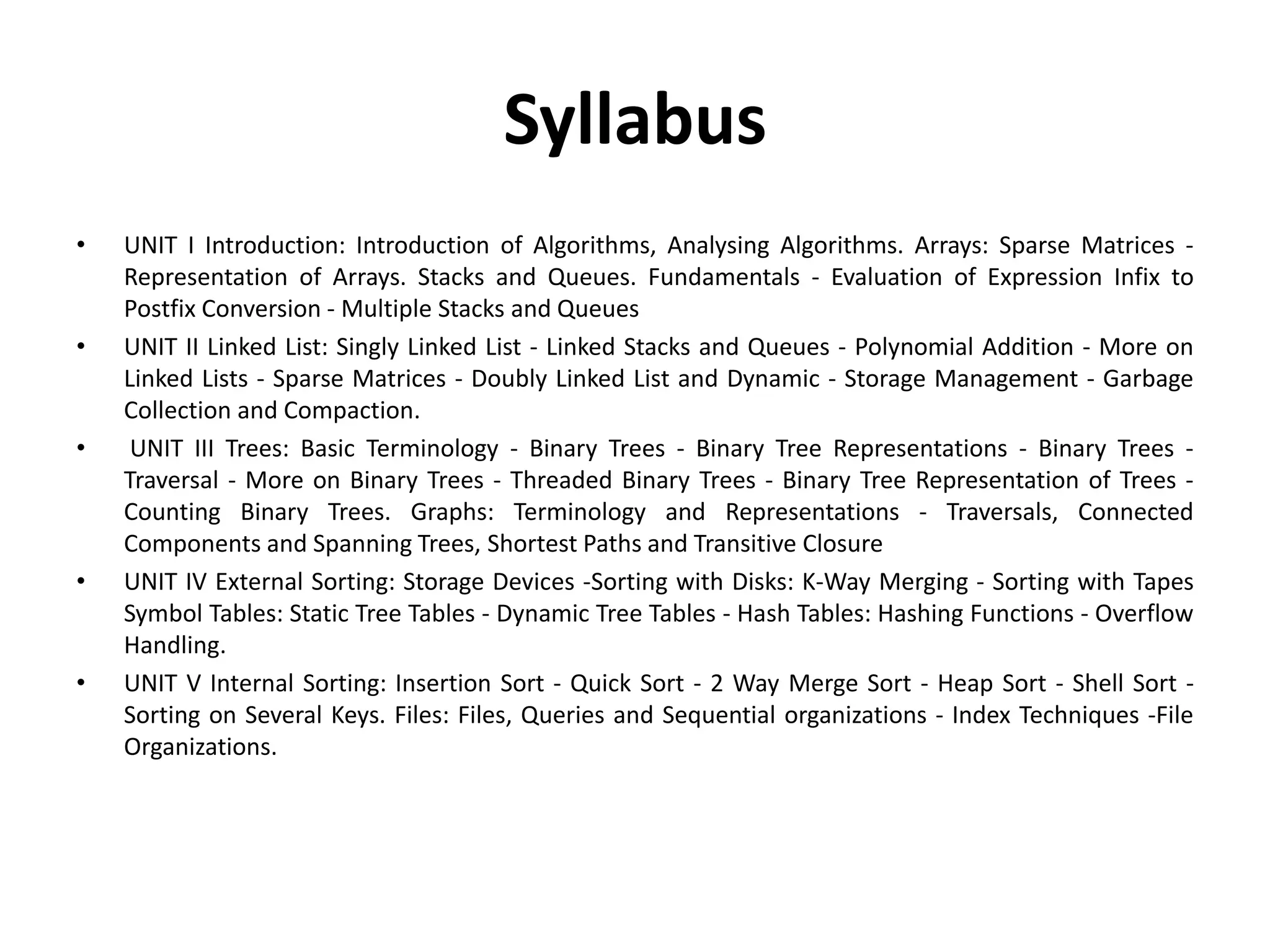
Syllabus • UNIT IIntroduction: Introduction of Algorithms, Analysing Algorithms. Arrays: Sparse Matrices - Representation of Arrays. Stacks and Queues. Fundamentals - Evaluation of Expression Infix to Postfix Conversion - Multiple Stacks and Queues • UNIT II Linked List: Singly Linked List - Linked Stacks and Queues - Polynomial Addition - More on Linked Lists - Sparse Matrices - Doubly Linked List and Dynamic - Storage Management - Garbage Collection and Compaction. • UNIT III Trees: Basic Terminology - Binary Trees - Binary Tree Representations - Binary Trees - Traversal - More on Binary Trees - Threaded Binary Trees - Binary Tree Representation of Trees - Counting Binary Trees. Graphs: Terminology and Representations - Traversals, Connected Components and Spanning Trees, Shortest Paths and Transitive Closure • UNIT IV External Sorting: Storage Devices -Sorting with Disks: K-Way Merging - Sorting with Tapes Symbol Tables: Static Tree Tables - Dynamic Tree Tables - Hash Tables: Hashing Functions - Overflow Handling. • UNIT V Internal Sorting: Insertion Sort - Quick Sort - 2 Way Merge Sort - Heap Sort - Shell Sort - Sorting on Several Keys. Files: Files, Queries and Sequential organizations - Index Techniques -File Organizations.
3.
Text Books TEXT BOOKS •1. Ellis Horowitz, Sartaj Shani, Data Structures, Galgotia Publication. • 2. Ellis Horowitz, Sartaj Shani, Sanguthevar Rajasekaran, Computer Algorithms, Galgotia Publication. • E-book - http://icodeguru.com/vc/10book/books/book 1/chap01.htm
4.
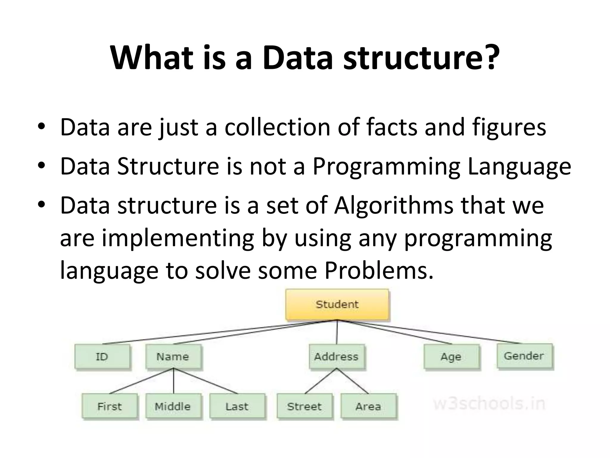
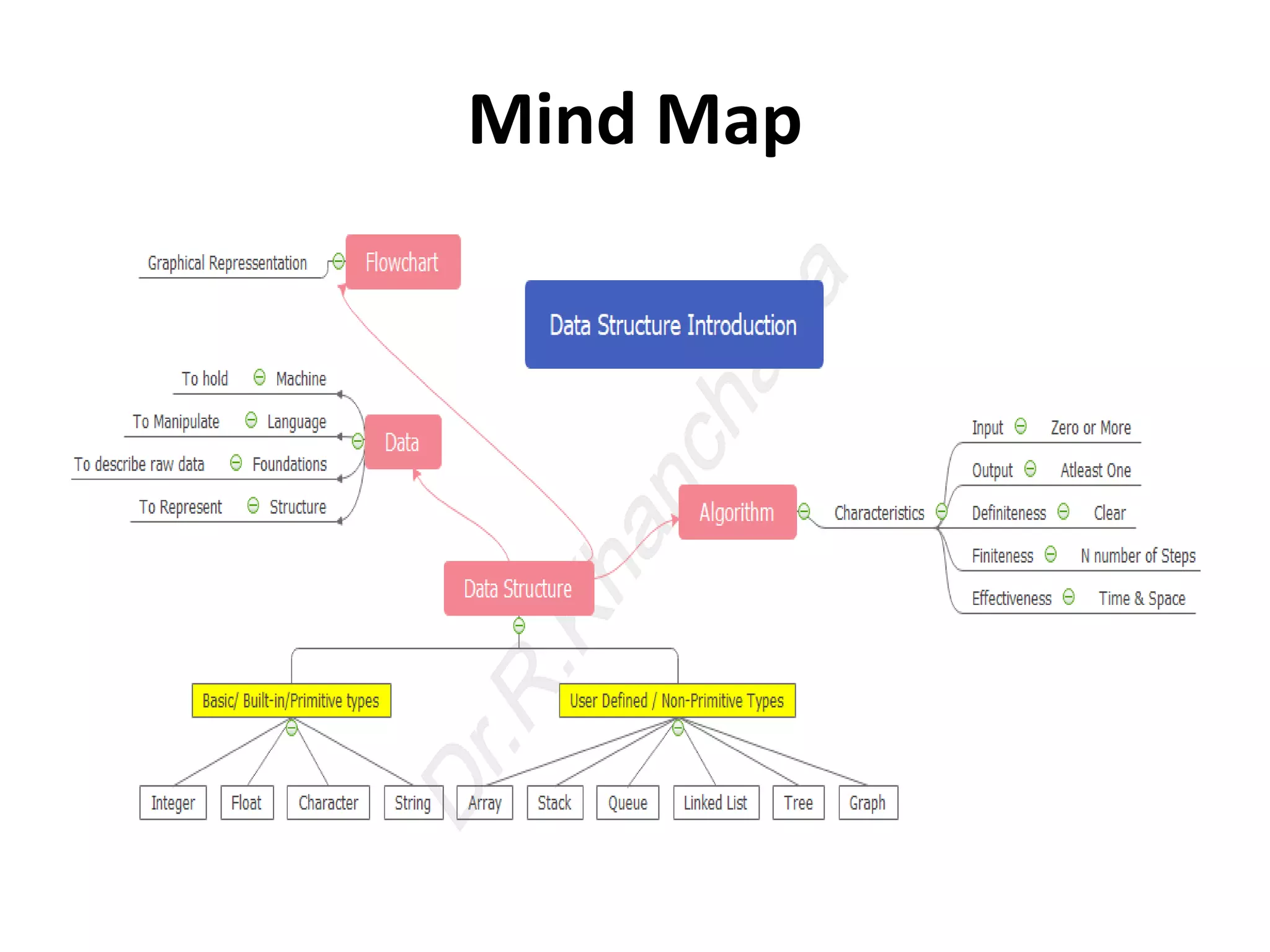
What is aData structure? • Data are just a collection of facts and figures • Data Structure is not a Programming Language • Data structure is a set of Algorithms that we are implementing by using any programming language to solve some Problems.
5.
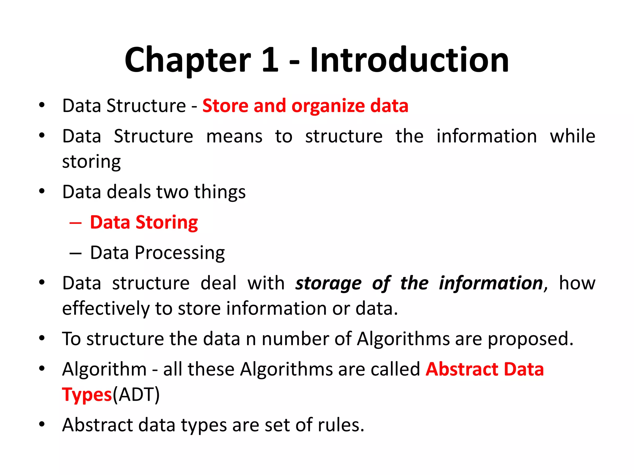
Chapter 1 -Introduction • Data Structure - Store and organize data • Data Structure means to structure the information while storing • Data deals two things – Data Storing – Data Processing • Data structure deal with storage of the information, how effectively to store information or data. • To structure the data n number of Algorithms are proposed. • Algorithm - all these Algorithms are called Abstract Data Types(ADT) • Abstract data types are set of rules.
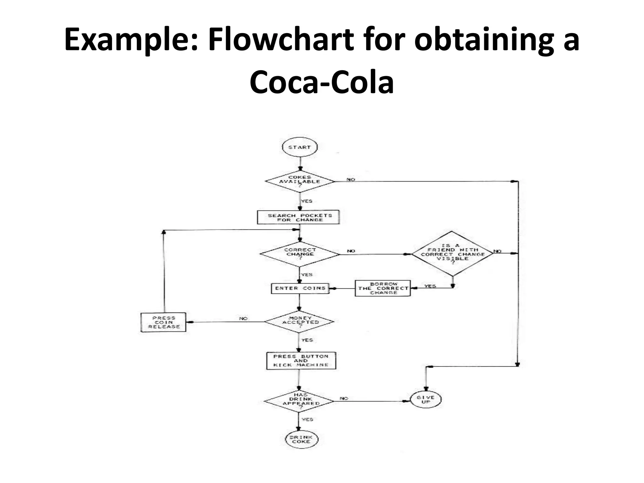
Algorithms - Overview •An algorithm is a procedure having well defined steps for solving a particular problem. • Definition: Algorithm is finite set of logic or instructions, written in order for accomplish the certain predefined task. • It is not the complete program or code, it is just a solution (logic) of a problem – Can be represented either as a Flowchart or Pseudo code.
10.
Study of Algorithms (i)machines for executing algorithms – From the smallest pocket calculator to the largest general purpose digital computer. (ii) languages for describing algorithms – language design and translation. (iii) foundations of algorithms – Particular task accomplishable by a computing device – What is the minimum number of operations necessary for any algorithm which performs a certain function? (iv) analysis of algorithms Performance is measured in terms of the computing time and space that are consumed while the algorithm is processing
11.
Characteristics of anAlgorithm • Input – There are zero or more quantities which are externally supplied • Output – At least one quantity is produced • Definiteness – Each instruction must be clear and unambiguous • Finiteness – If trace out the instructions of an algorithm, then for all cases the algorithm will terminate after a finite number of steps • Effectiveness – Time & Space – Every instruction must be sufficiently basic and also be feasible.
12.
Flowchart • Raw datais input and algorithms are used to transform it into refined data. So, instead of saying that computer science is the study of algorithms, alternatively, it is the study of data: • (i) machines that hold data; • (ii) languages for describing data manipulation; • (iii) foundations which describe what kinds of refined data can be produced from raw data; • (iv) structures for representing data.
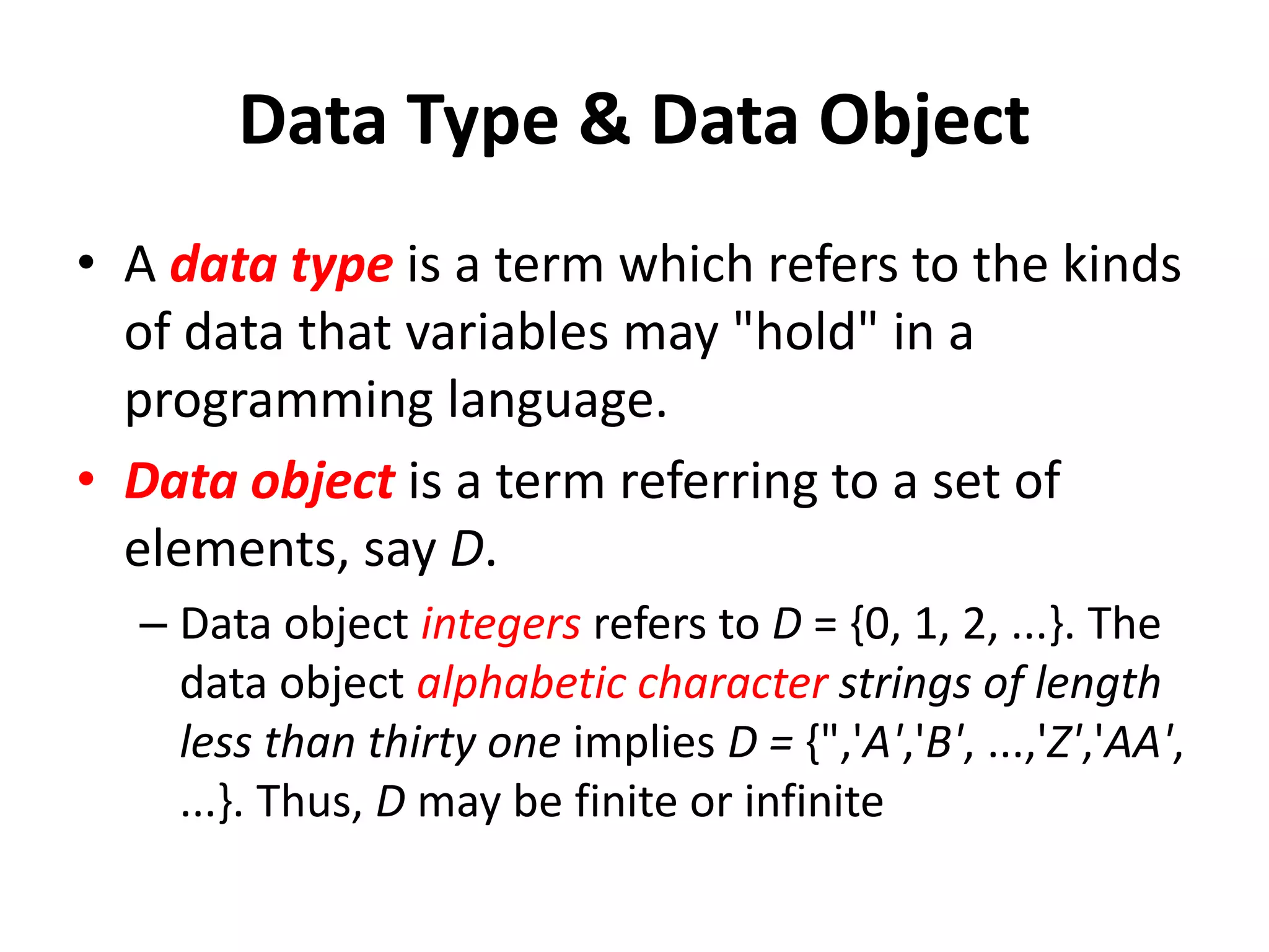
Data Type &Data Object • A data type is a term which refers to the kinds of data that variables may "hold" in a programming language. • Data object is a term referring to a set of elements, say D. – Data object integers refers to D = {0, 1, 2, ...}. The data object alphabetic character strings of length less than thirty one implies D = {",'A','B', ...,'Z','AA', ...}. Thus, D may be finite or infinite
How to Analyze Programs/Algorithms? Thereare many criteria upon which judge a program, for instance: • (i) Does it do what we want it to do? • (ii) Does it work correctly according to the original specifications of the task? • (iii) Is there documentation which describes how to use it and how it works? • (iv) Are subroutines created in such a way that they perform logical sub-functions? • (v) Is the code readable?
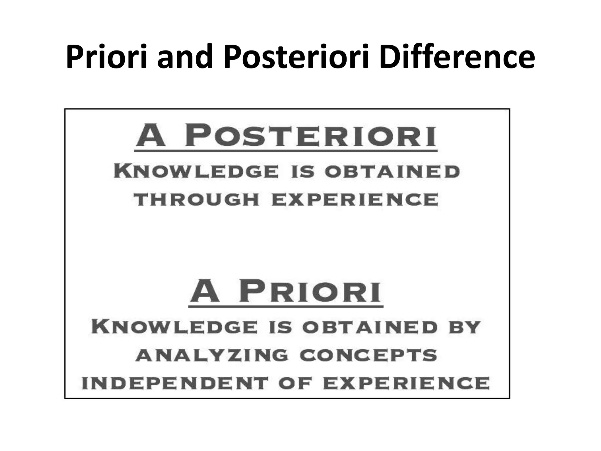
Performance evaluation • Performanceevaluation can be divided into 2 major phases: – (a) a priori estimates and – (b) a posteriori testing. Both of these are equally important. • First consider a priori estimation. Suppose that somewhere in one of your programs is the statement • x = x + 1
24.
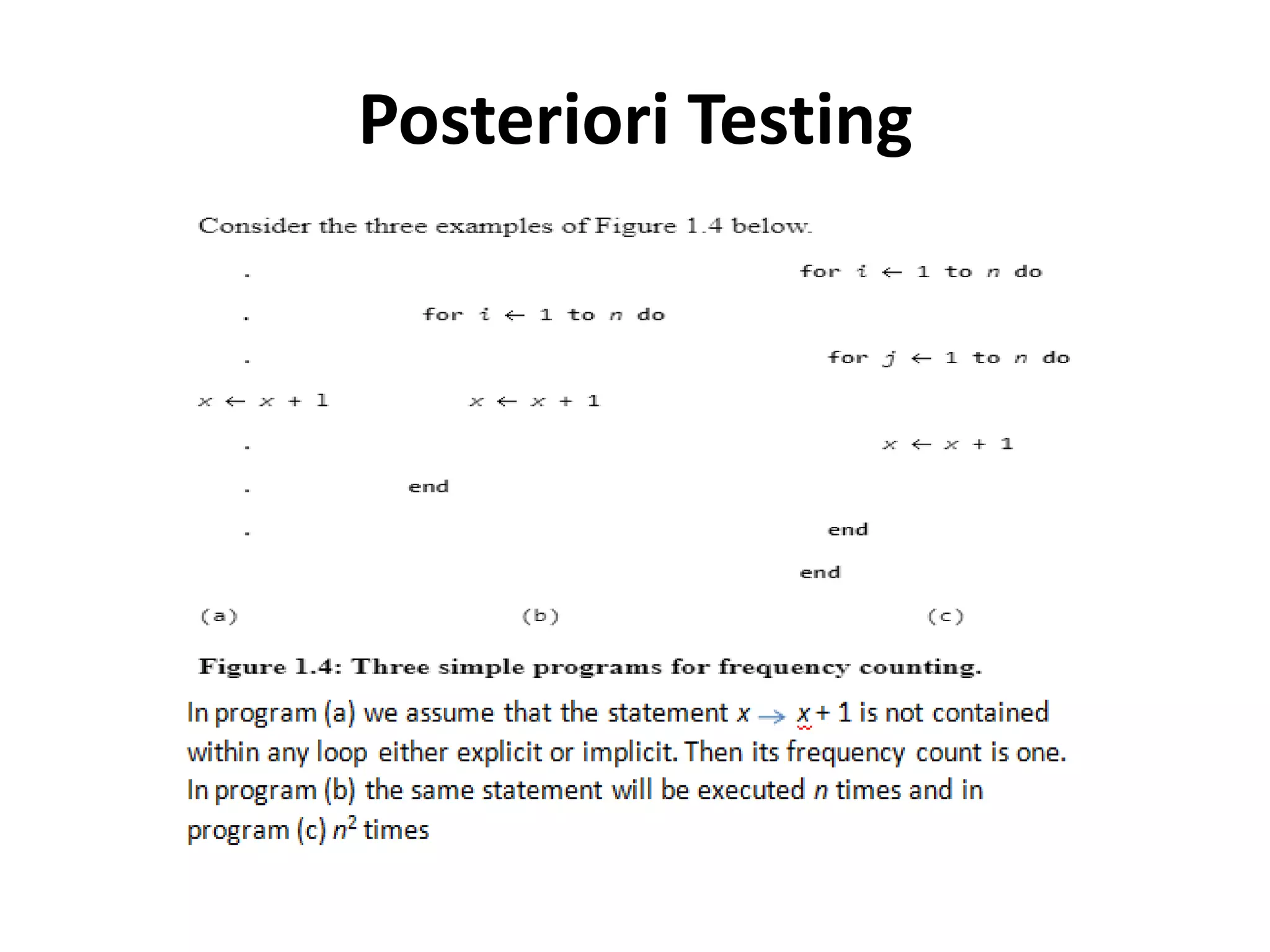
Performance evaluation Time Complexity –first is the amount of time a single execution will take – second is the number of times it is executed. • The product of these numbers will be the total time taken by this statement. • The second statistic is called the frequency count, and this may vary from data set to data set.
25.
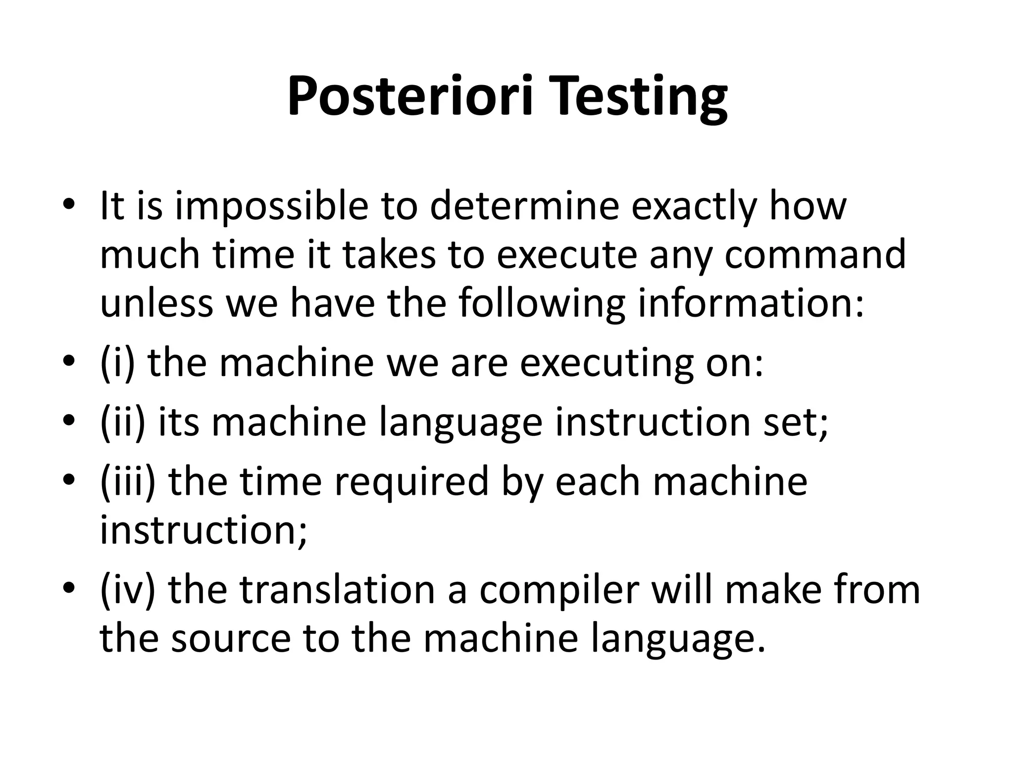
Posteriori Testing • Itis impossible to determine exactly how much time it takes to execute any command unless we have the following information: • (i) the machine we are executing on: • (ii) its machine language instruction set; • (iii) the time required by each machine instruction; • (iv) the translation a compiler will make from the source to the machine language.
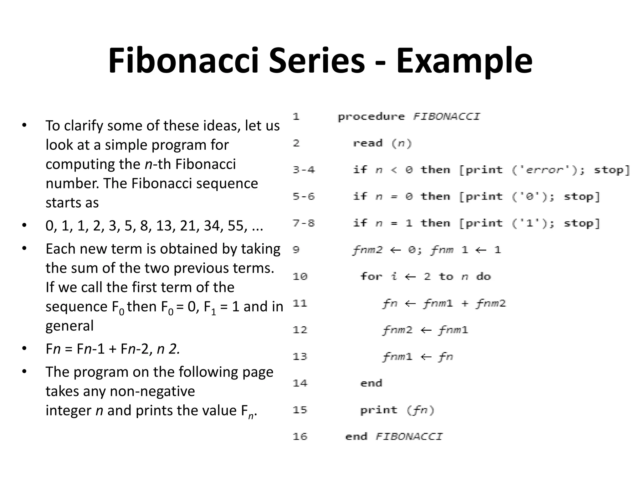
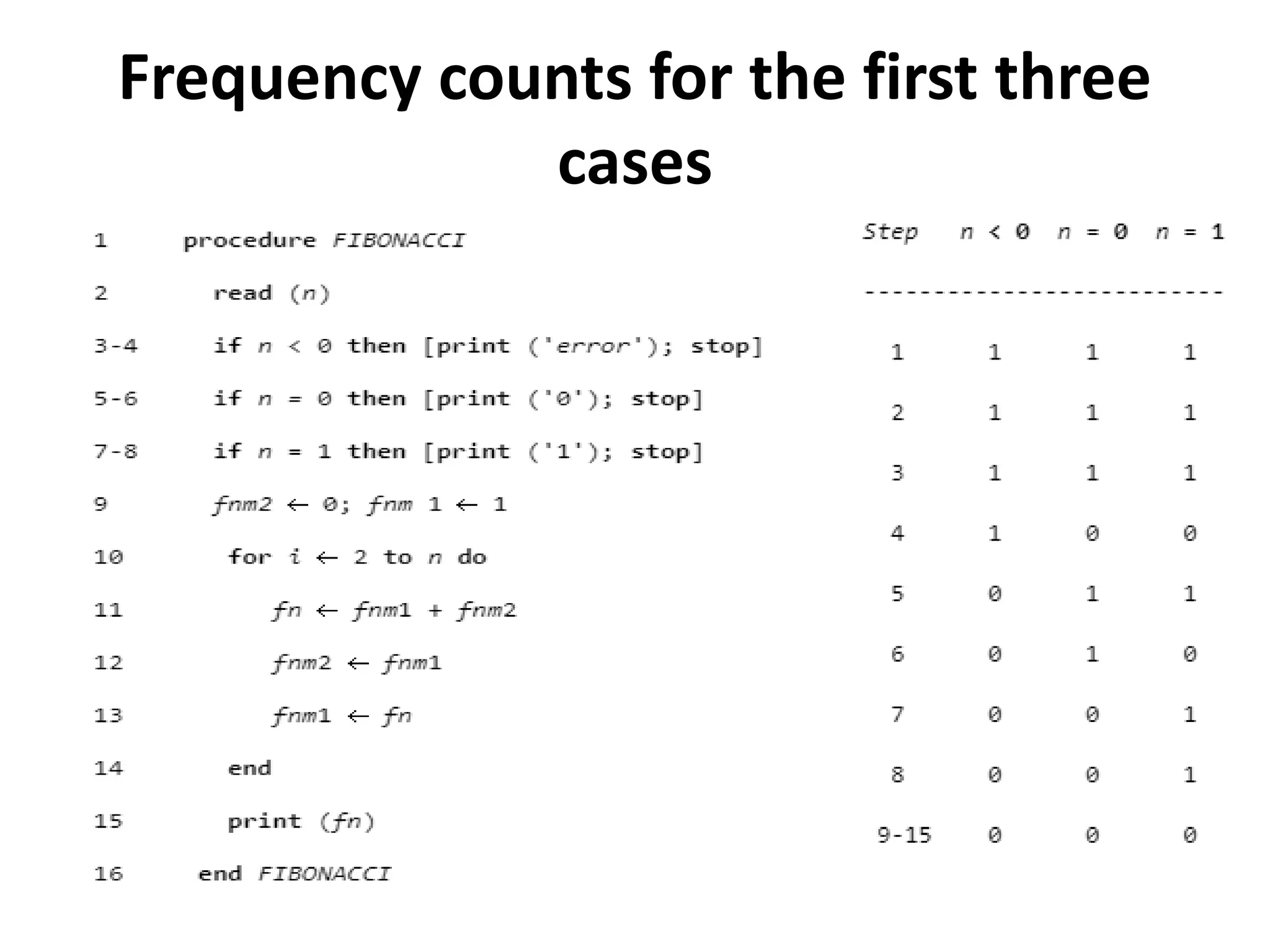
Fibonacci Series -Example • To clarify some of these ideas, let us look at a simple program for computing the n-th Fibonacci number. The Fibonacci sequence starts as • 0, 1, 1, 2, 3, 5, 8, 13, 21, 34, 55, ... • Each new term is obtained by taking the sum of the two previous terms. If we call the first term of the sequence F0 then F0 = 0, F1 = 1 and in general • Fn = Fn-1 + Fn-2, n 2. • The program on the following page takes any non-negative integer n and prints the value Fn.
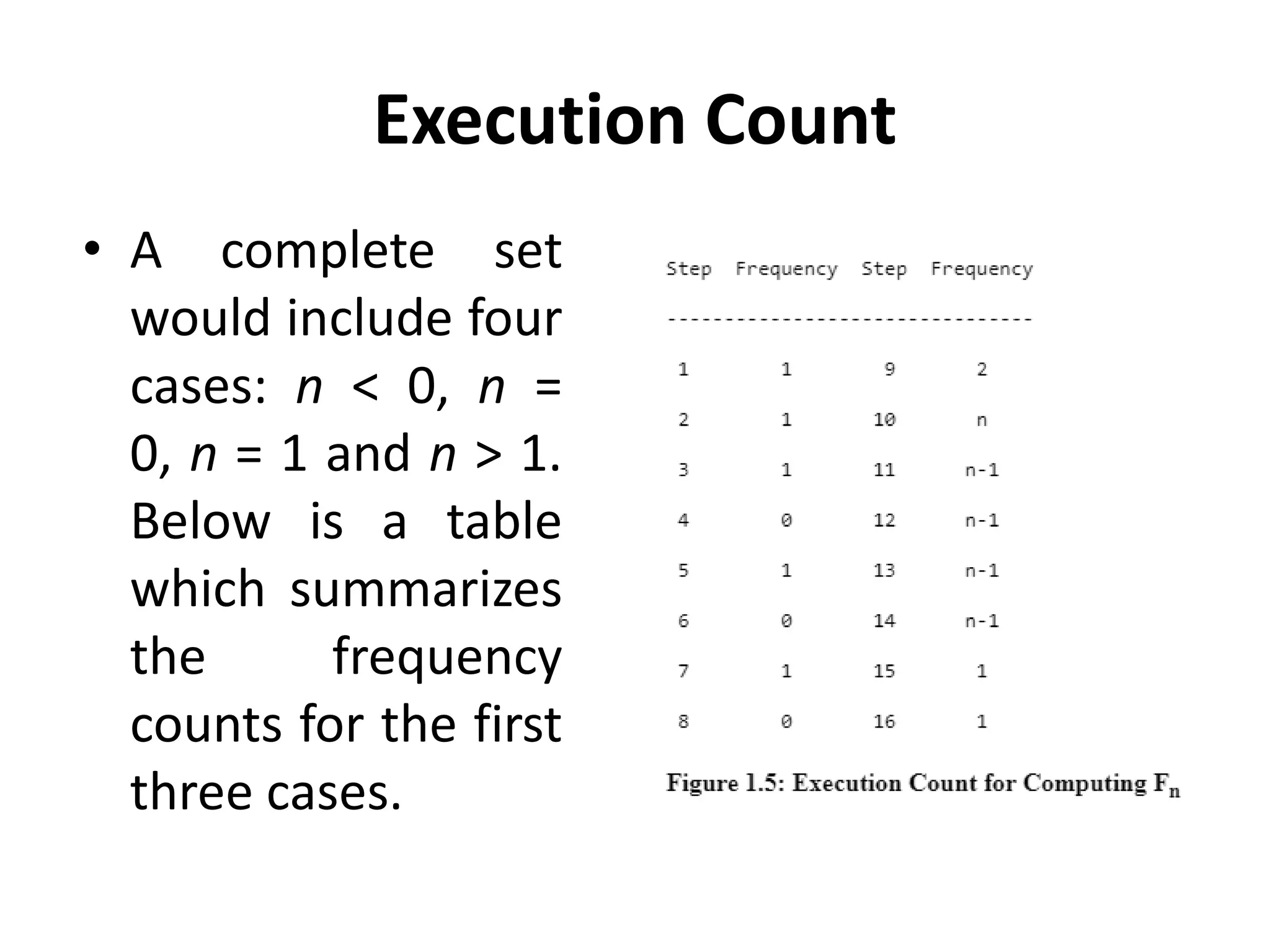
Execution Count • Acomplete set would include four cases: n < 0, n = 0, n = 1 and n > 1. Below is a table which summarizes the frequency counts for the first three cases.
31.
Time Computation • Forexample n might be the number of inputs or the number of outputs or their sum or the magnitude of one of them. For the Fibonacci program n represents the magnitude of the input and the time for this program is written as T(FIBONACCI) = O(n).
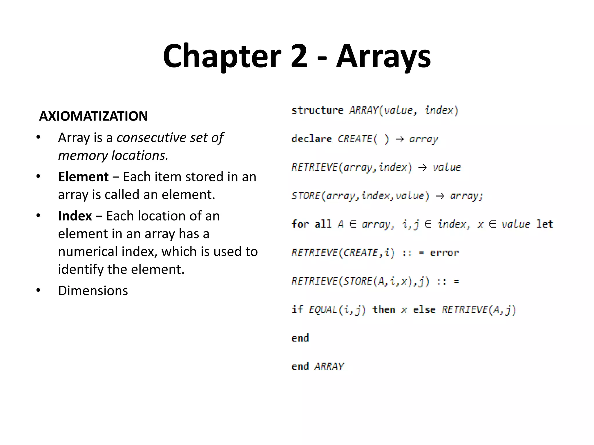
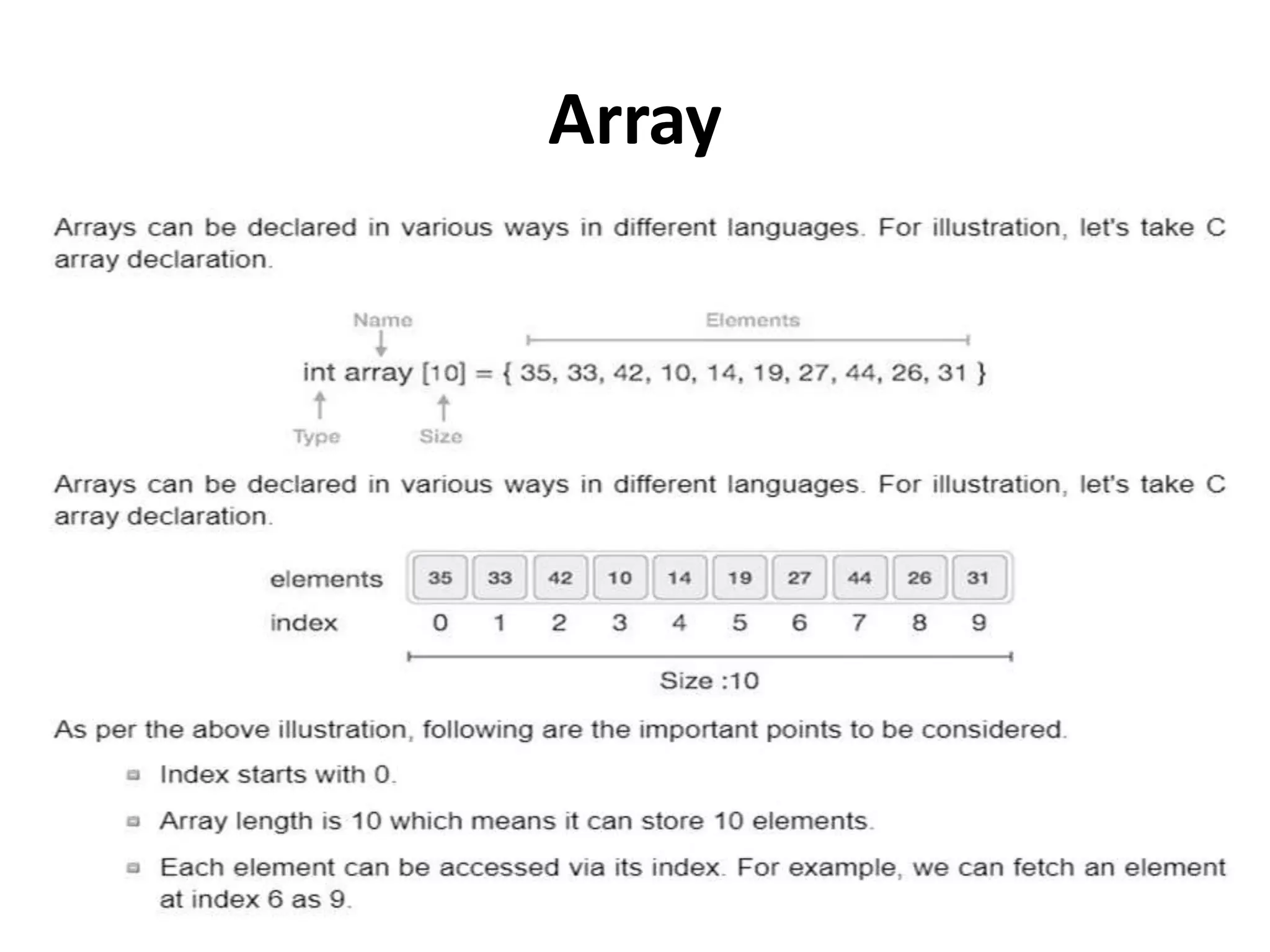
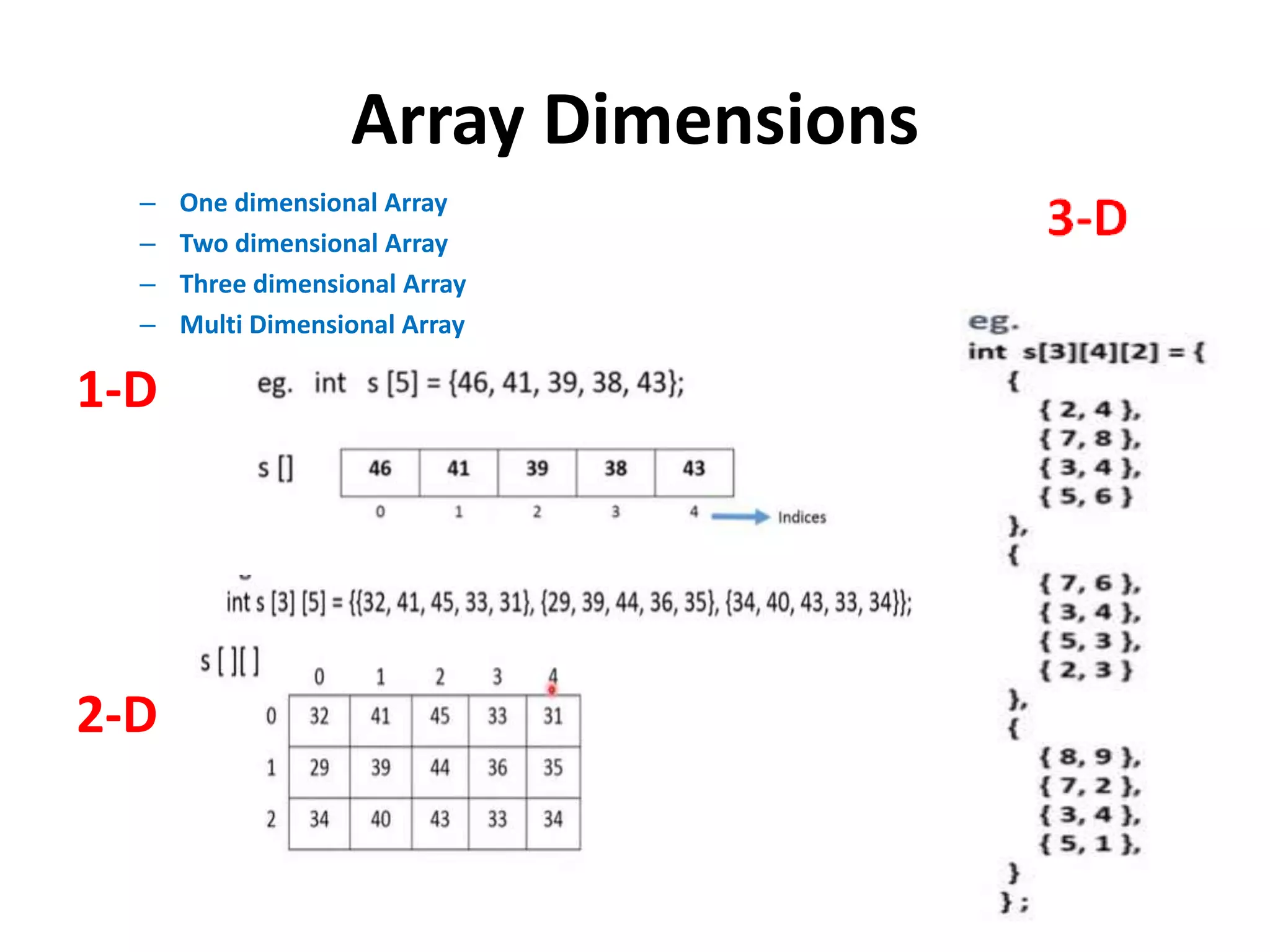
Chapter 2 -Arrays AXIOMATIZATION • Array is a consecutive set of memory locations. • Element − Each item stored in an array is called an element. • Index − Each location of an element in an array has a numerical index, which is used to identify the element. • Dimensions
Array Dimensions – Onedimensional Array – Two dimensional Array – Three dimensional Array – Multi Dimensional Array 1-D 2-D
38.
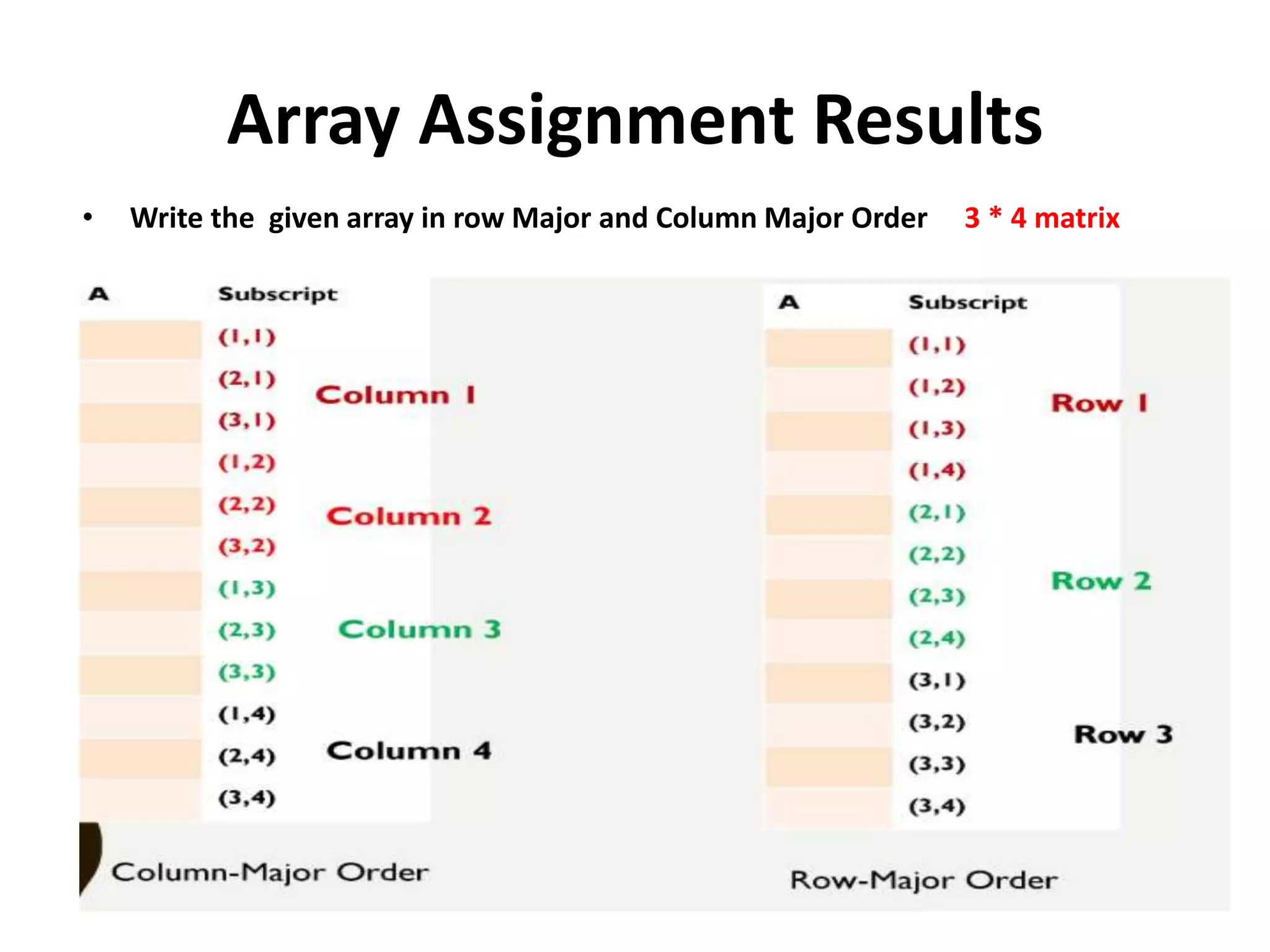
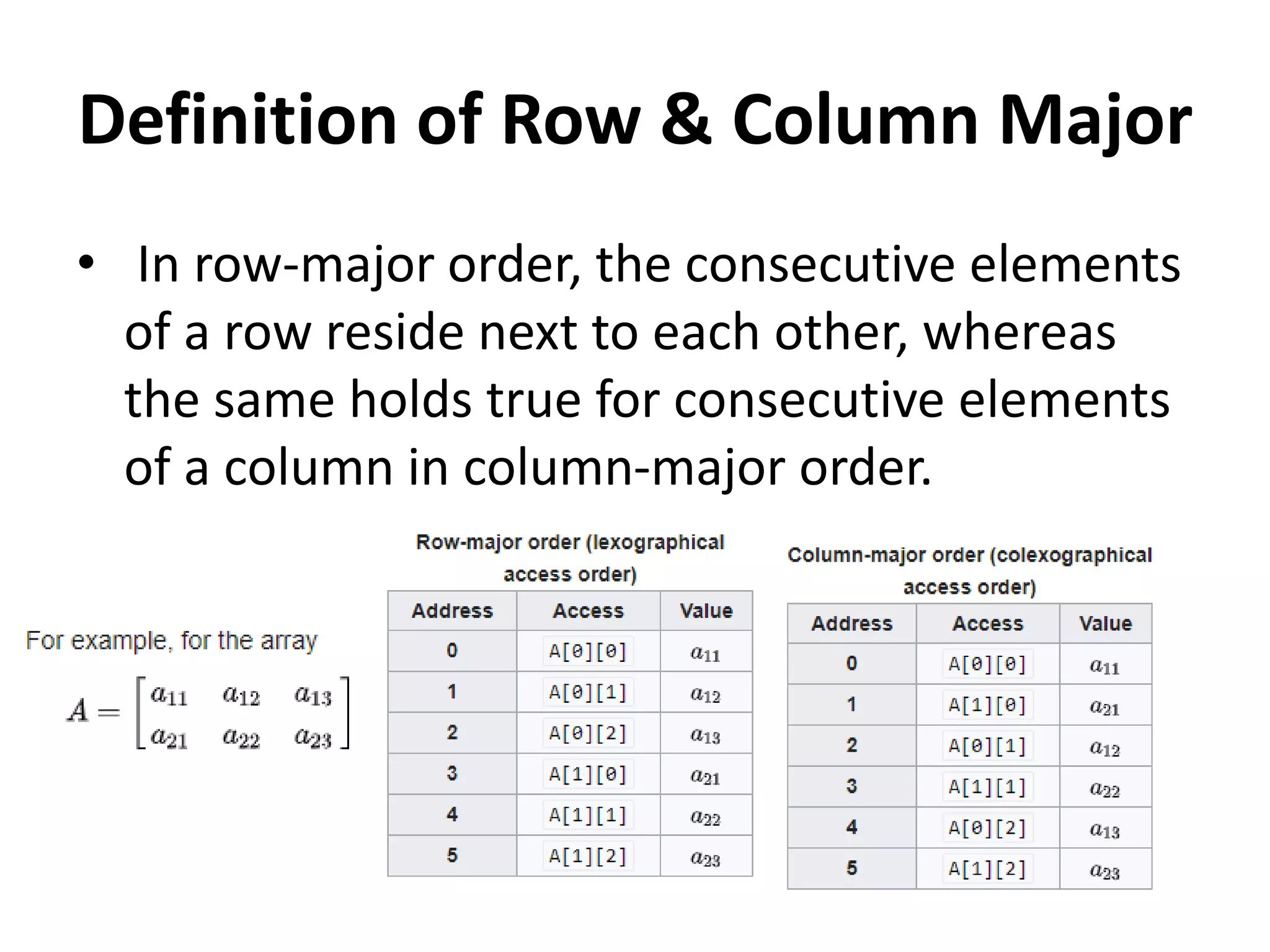
Definition of Row& Column Major • In row-major order, the consecutive elements of a row reside next to each other, whereas the same holds true for consecutive elements of a column in column-major order.
39.
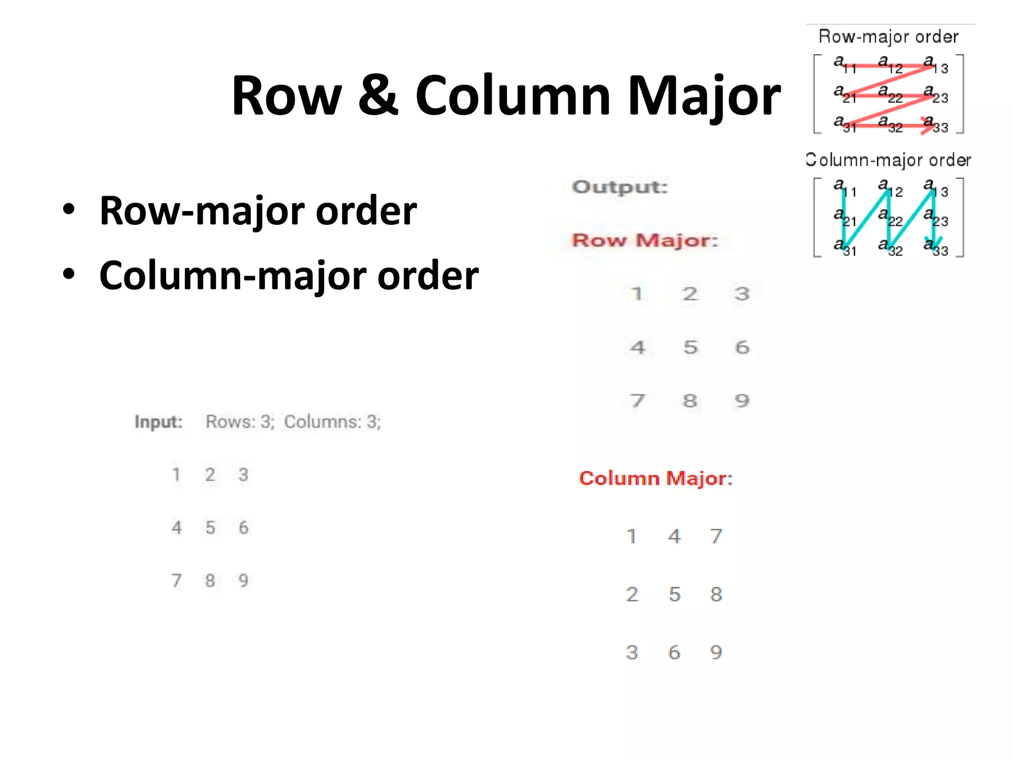
Row & ColumnMajor • Row-major order • Column-major order
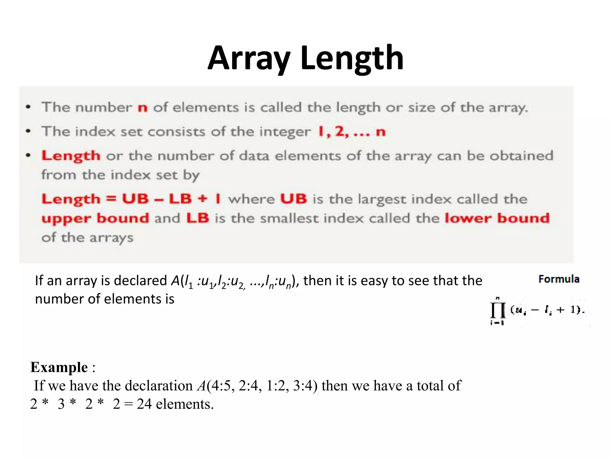
Array Length If anarray is declared A(l1 :u1,l2:u2, ...,ln:un), then it is easy to see that the number of elements is Example : If we have the declaration A(4:5, 2:4, 1:2, 3:4) then we have a total of 2 * 3 * 2 * 2 = 24 elements.
42.
Array Length -Example •1-D A[5..12] • Formula - Ui-li+1 • Elements are • U,B,F,D,A,E,C • 7-0+1 • 6 • 2-D A[0..2]B[0..3] • Formula - (U1-l1+1) * (U2-l2+1) • Array Size • =(2-0+1)*(3-0+1) = 3 *4 = 12 SIZE
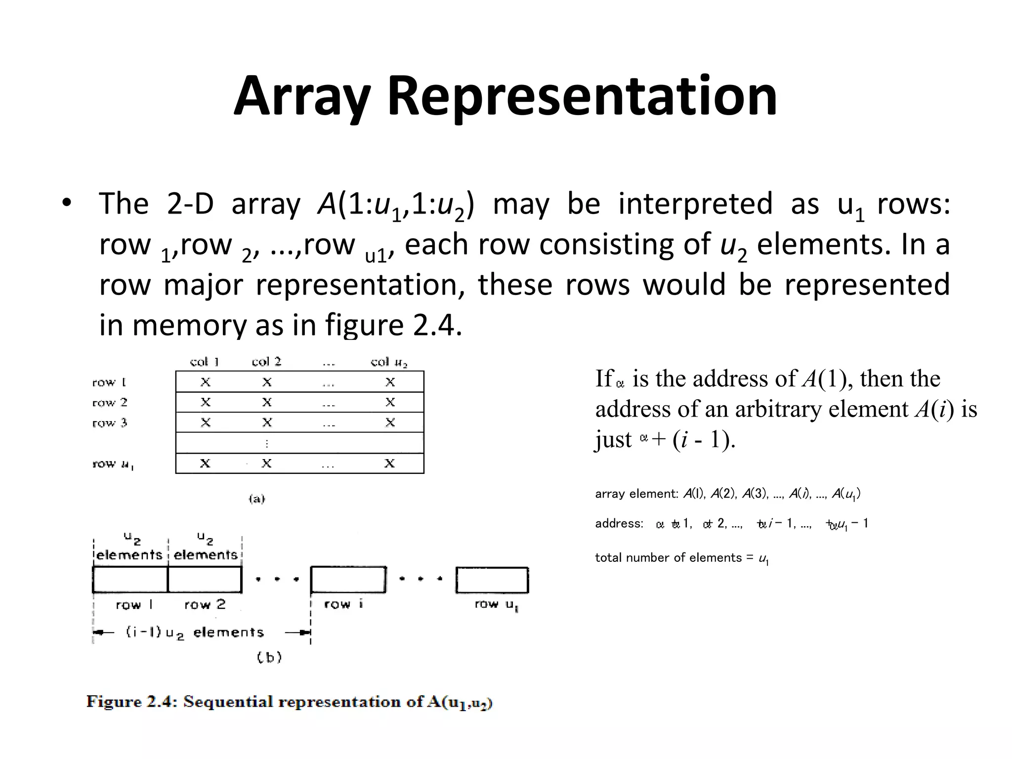
Array Representation • The2-D array A(1:u1,1:u2) may be interpreted as u1 rows: row 1,row 2, ...,row u1, each row consisting of u2 elements. In a row major representation, these rows would be represented in memory as in figure 2.4. If is the address of A(1), then the address of an arbitrary element A(i) is just + (i - 1). array element: A(l), A(2), A(3), ..., A(i), ..., A(u1) address: , + 1, + 2, ..., + i - 1, ..., + u1 - 1 total number of elements = u1
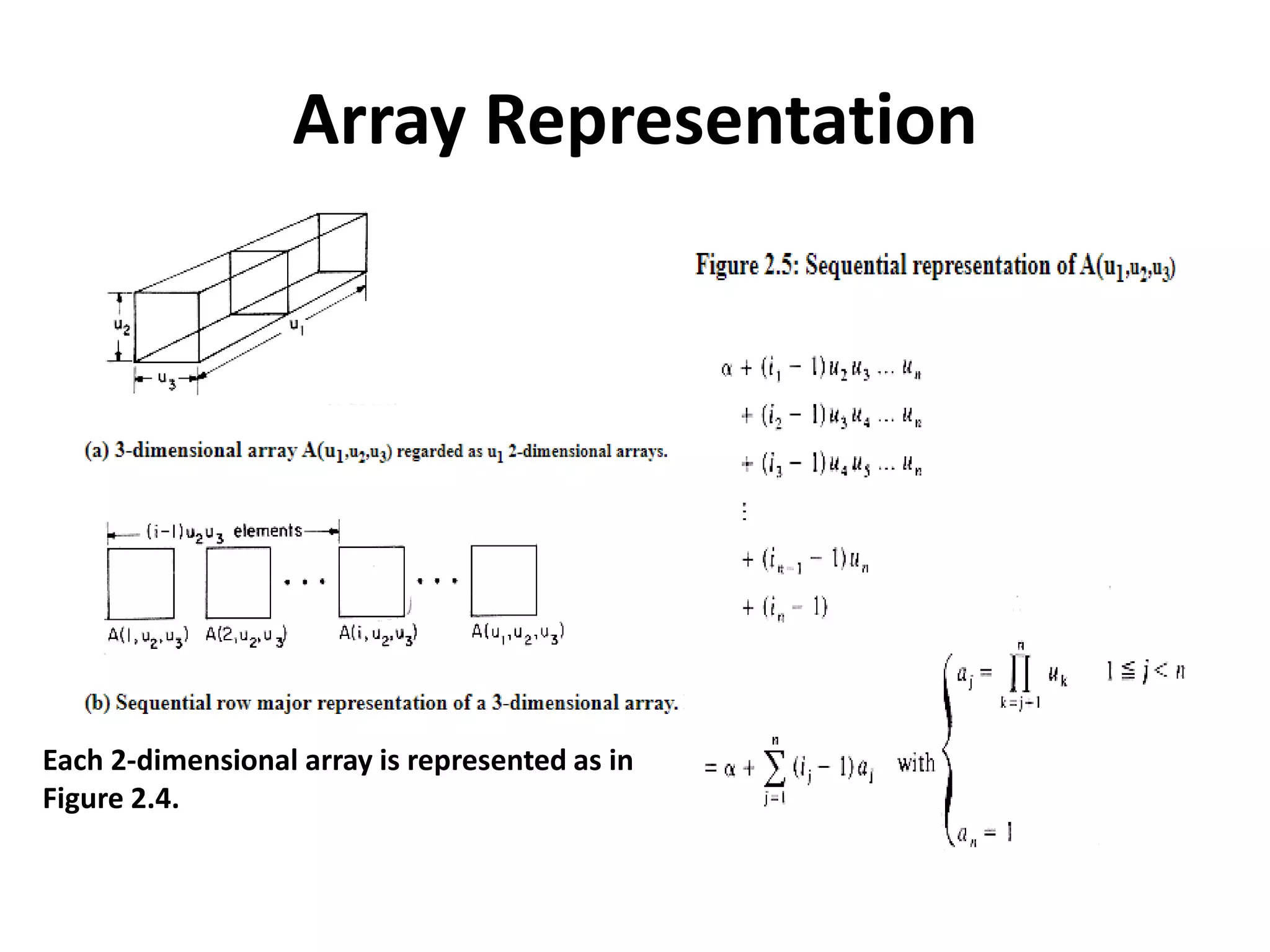
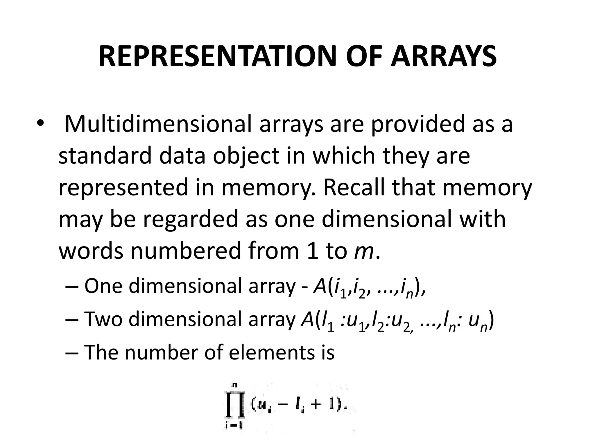
REPRESENTATION OF ARRAYS •Multidimensional arrays are provided as a standard data object in which they are represented in memory. Recall that memory may be regarded as one dimensional with words numbered from 1 to m. – One dimensional array - A(i1,i2, ...,in), – Two dimensional array A(l1 :u1,l2:u2, ...,ln: un) – The number of elements is
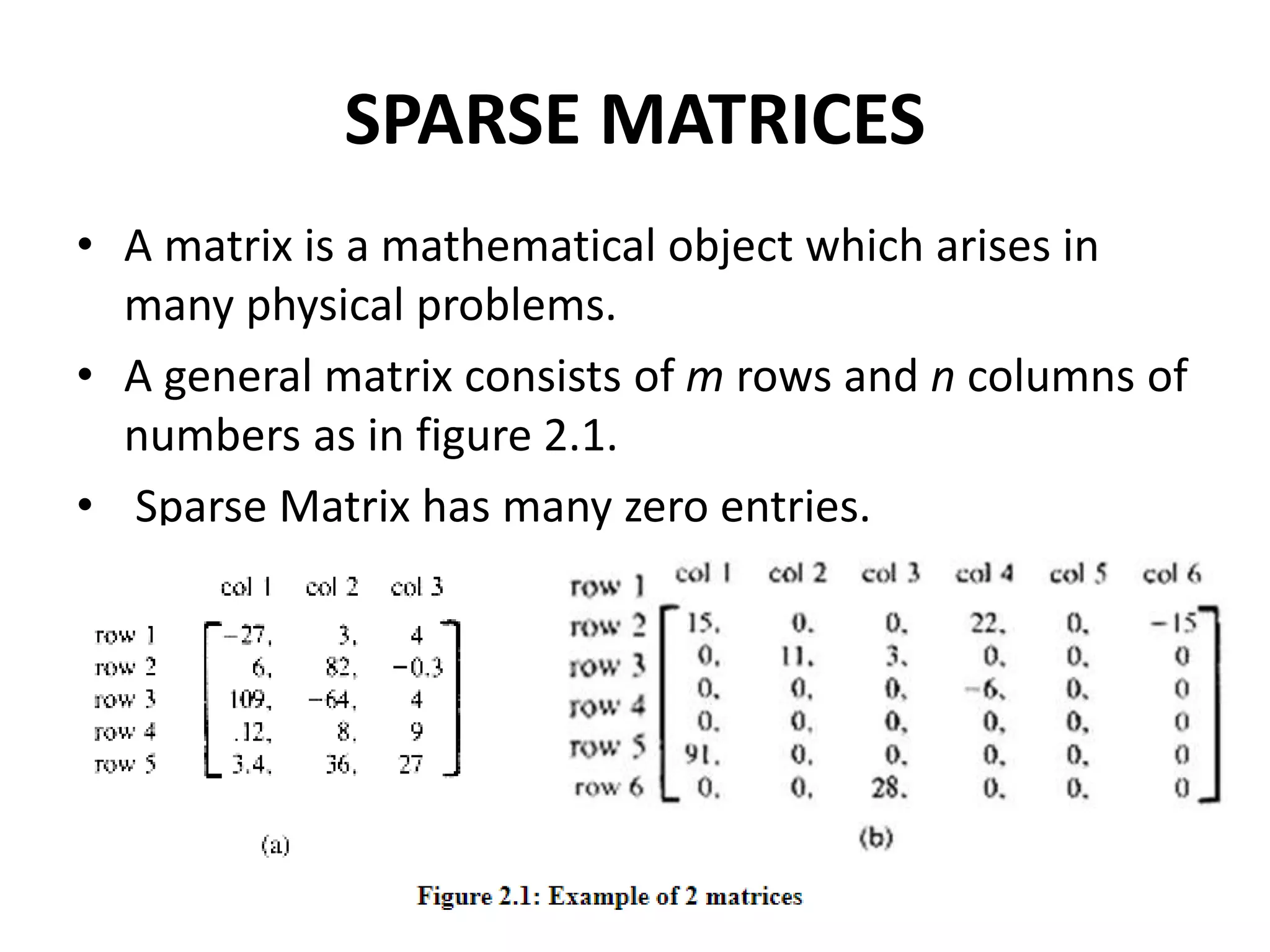
SPARSE MATRICES • Amatrix is a mathematical object which arises in many physical problems. • A general matrix consists of m rows and n columns of numbers as in figure 2.1. • Sparse Matrix has many zero entries.
52.
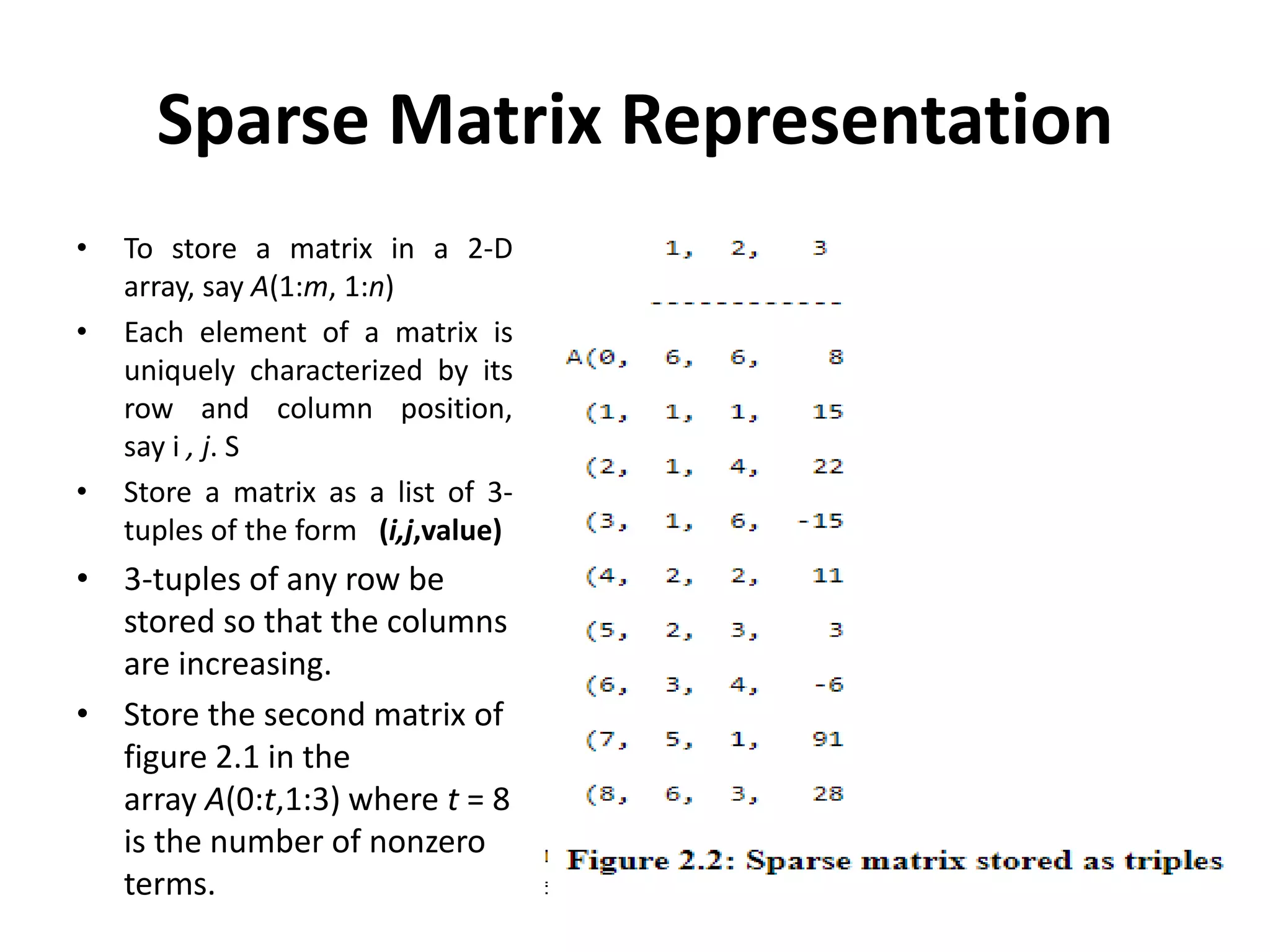
Sparse Matrix Representation •To store a matrix in a 2-D array, say A(1:m, 1:n) • Each element of a matrix is uniquely characterized by its row and column position, say i , j. S • Store a matrix as a list of 3- tuples of the form (i,j,value) • 3-tuples of any row be stored so that the columns are increasing. • Store the second matrix of figure 2.1 in the array A(0:t,1:3) where t = 8 is the number of nonzero terms.
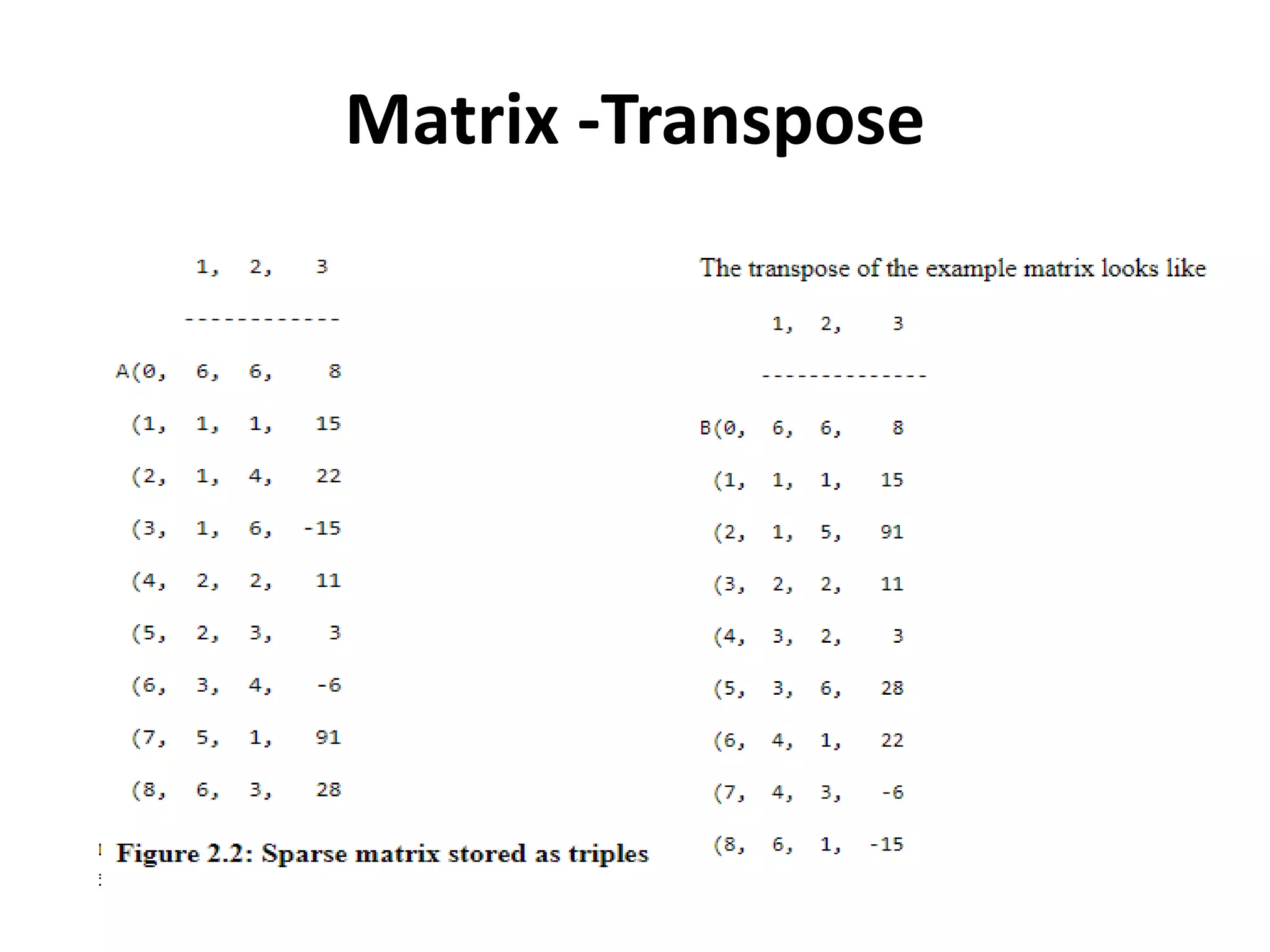
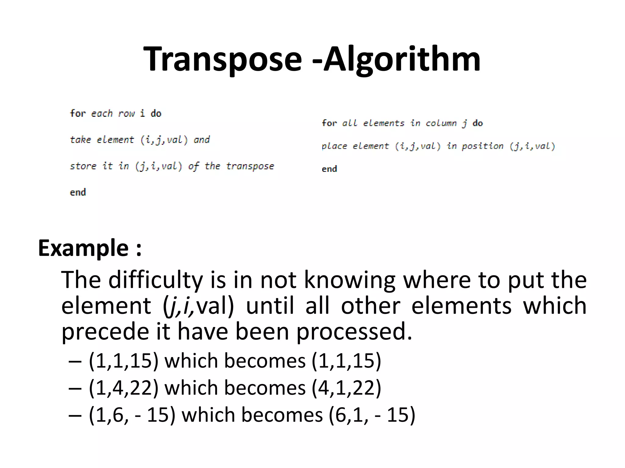
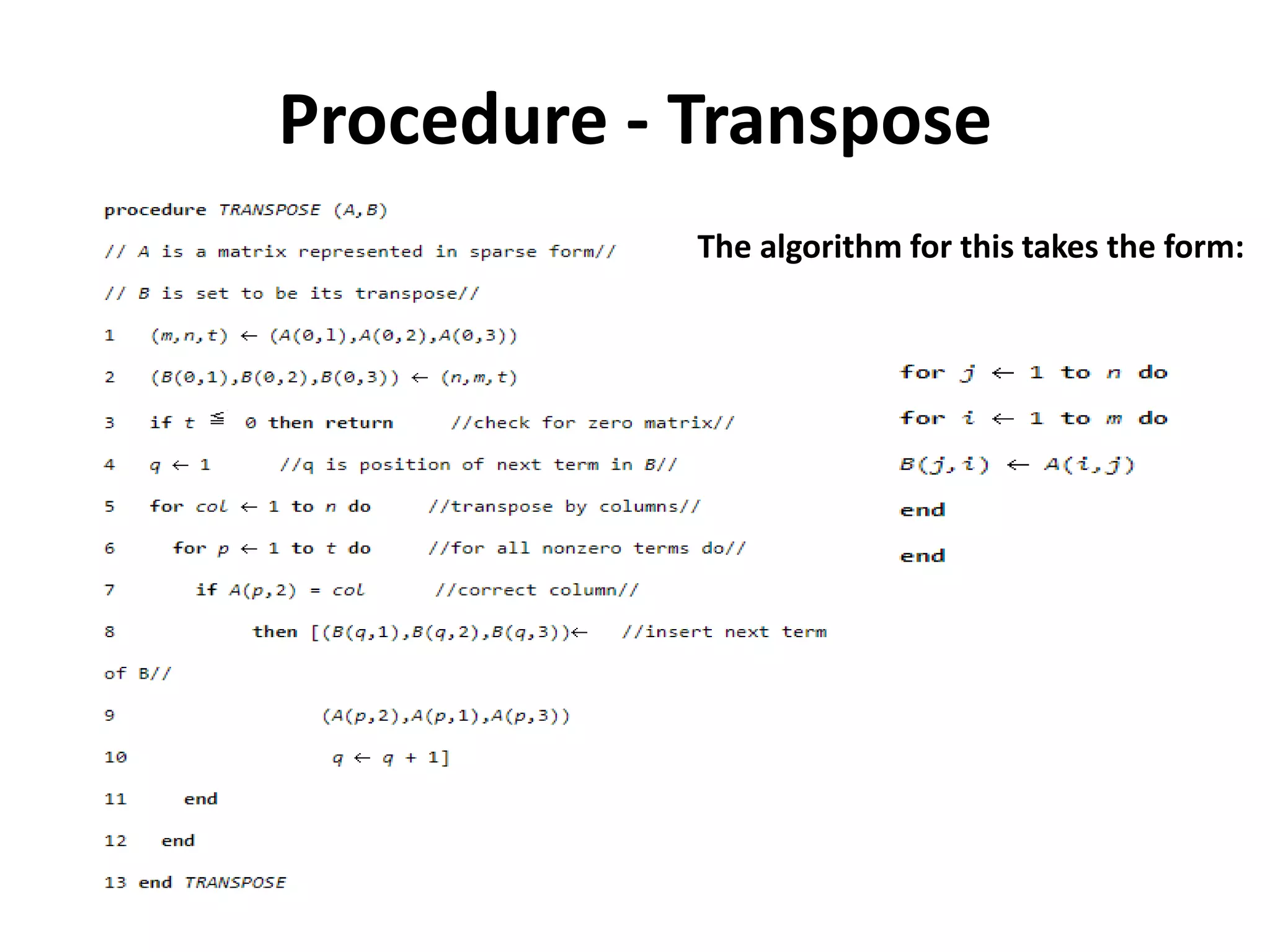
Transpose -Algorithm Example : Thedifficulty is in not knowing where to put the element (j,i,val) until all other elements which precede it have been processed. – (1,1,15) which becomes (1,1,15) – (1,4,22) which becomes (4,1,22) – (1,6, - 15) which becomes (6,1, - 15)
![Array Length -Example • 1-D A[5..12] • Formula - Ui-li+1 • Elements are • U,B,F,D,A,E,C • 7-0+1 • 6 • 2-D A[0..2]B[0..3] • Formula - (U1-l1+1) * (U2-l2+1) • Array Size • =(2-0+1)*(3-0+1) = 3 *4 = 12 SIZE](https://image.slidesharecdn.com/uniti-datastructuresintoduction-200713093528/75/Unit-I-Data-structures-Introduction-Evaluation-of-Algorithms-Arrays-Sparse-Matrix-42-2048.jpg)
![Array Memory Allocation 2-D array b[i][j] 1-D array a[10]](https://image.slidesharecdn.com/uniti-datastructuresintoduction-200713093528/75/Unit-I-Data-structures-Introduction-Evaluation-of-Algorithms-Arrays-Sparse-Matrix-43-2048.jpg)