Download to read offline

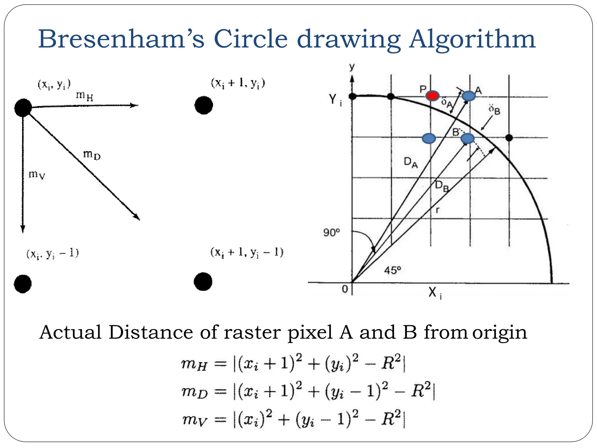
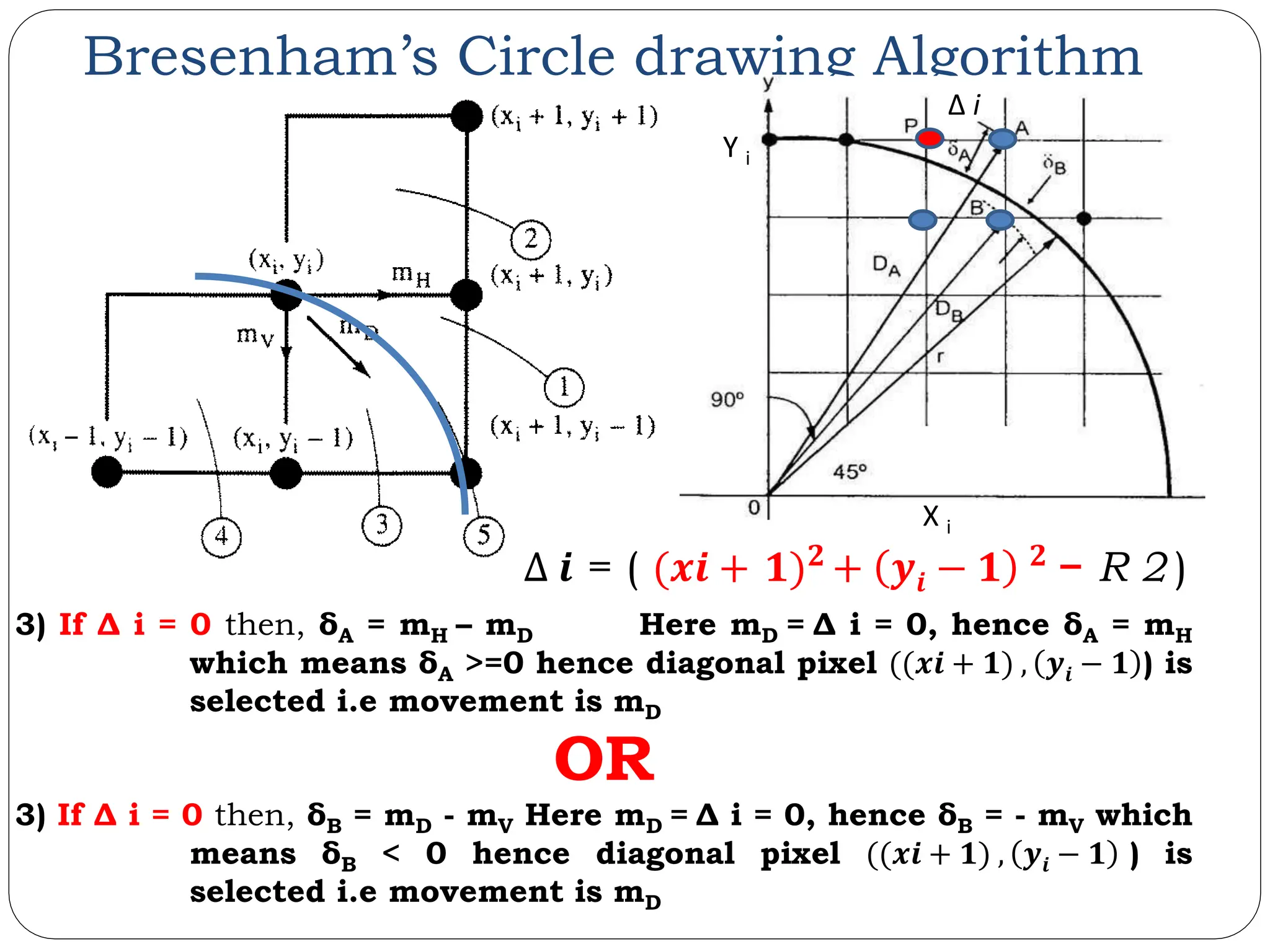
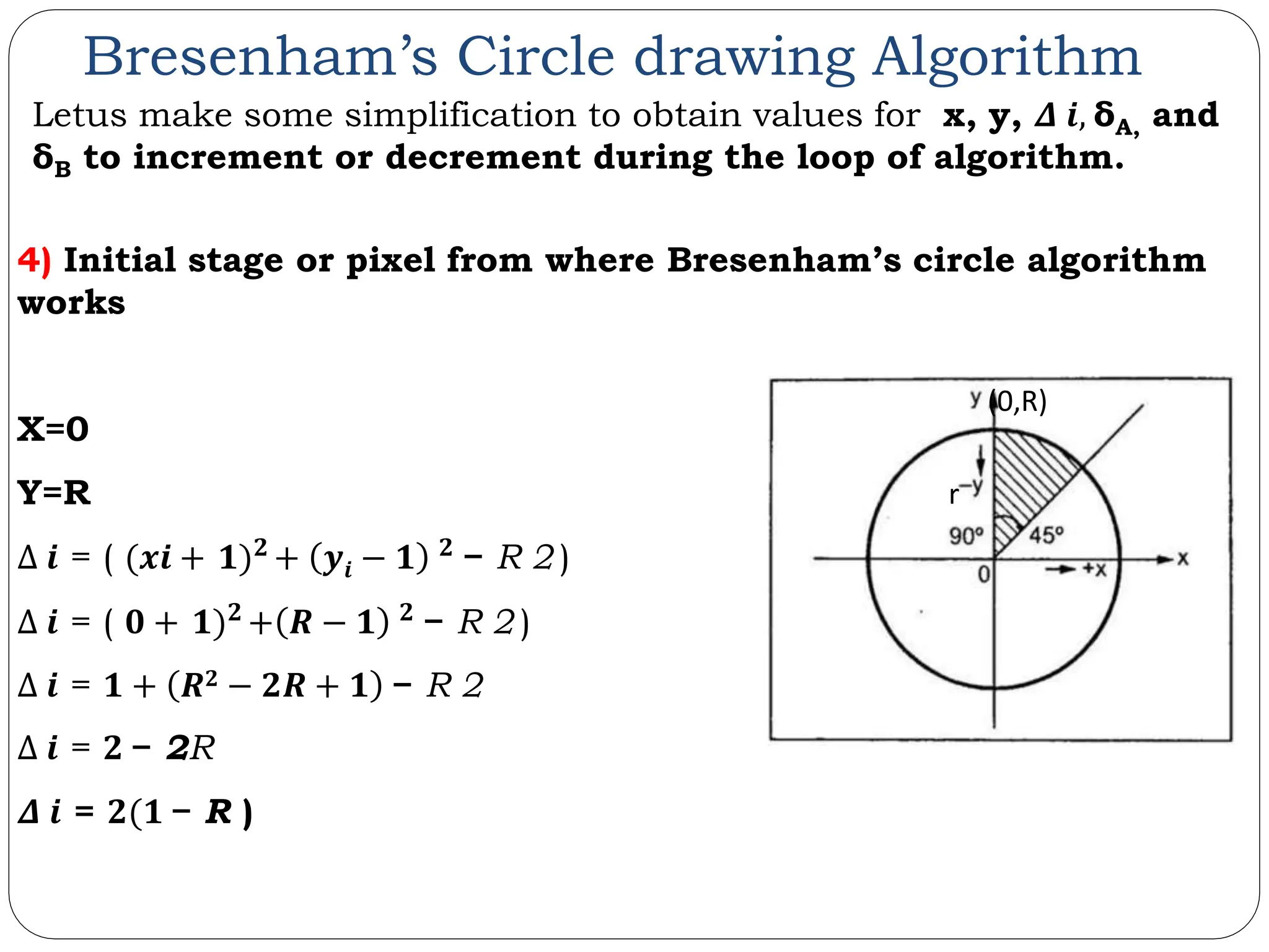
![Bresenham’s Circle drawing Algorithm Let us simplify, δA = mH - mD 𝝏𝑨 = | (𝒙𝒊 + 𝟏)𝟐 + 𝒚𝒊 𝟐 - R 2 | - | ( (𝒙𝒊 + 𝟏)𝟐 + 𝒚𝒊 − 𝟏 𝟐 - R 2 ) | 𝜕𝐴 = | ( (𝑥𝑖 + 1)2 + 𝒚𝒊 − 𝟏 𝟐 − R 2 ) | - | ( (𝑥𝑖 + 1)2 + 𝒚𝒊 − 𝟏 𝟐 - R 2) |+ (2𝒚𝒊 + 1) 𝜕𝐴 = 2| ( (𝑥𝑖 + 1)2 + 𝒚𝒊 − 𝟏 𝟐 − R 2 ) | + 2𝒚𝒊 + 1 𝜕𝐴 = 𝟐Δ 𝒊 + 2𝒚𝒊 + 1 𝜕𝐴 = | (𝑥𝑖 + 1)2 + 𝒚𝒊 2 − 2𝒚𝒊 - 1 - R 2 | - | ( (𝑥𝑖 + 1)2 + 𝑦𝑖 − 1 2 - R 2) |+ (2𝒚𝒊 + 1) 𝜕𝐴 = 𝟐 ( 𝜟 𝒊 + 𝒚𝒊 ) + 1 ---------[ III ] 𝜕𝐴 = | (𝑥𝑖 + 1)2 + 𝒚𝒊 2 − (2𝒚𝒊 + 1) - R 2 | - | ( (𝑥𝑖 + 1)2 + 𝑦𝑖 − 1 2 - R 2) |+ (2𝒚𝒊+1) Δ 𝒊 = ( (𝒙𝒊 + 𝟏)𝟐 + 𝒚𝒊 − 𝟏 𝟐 − R 2 )](https://image.slidesharecdn.com/unit-2rasterscangraphics-240510102813-03304cf8/75/Study-on-Fundamentals-of-Raster-Scan-Graphics-33-2048.jpg)
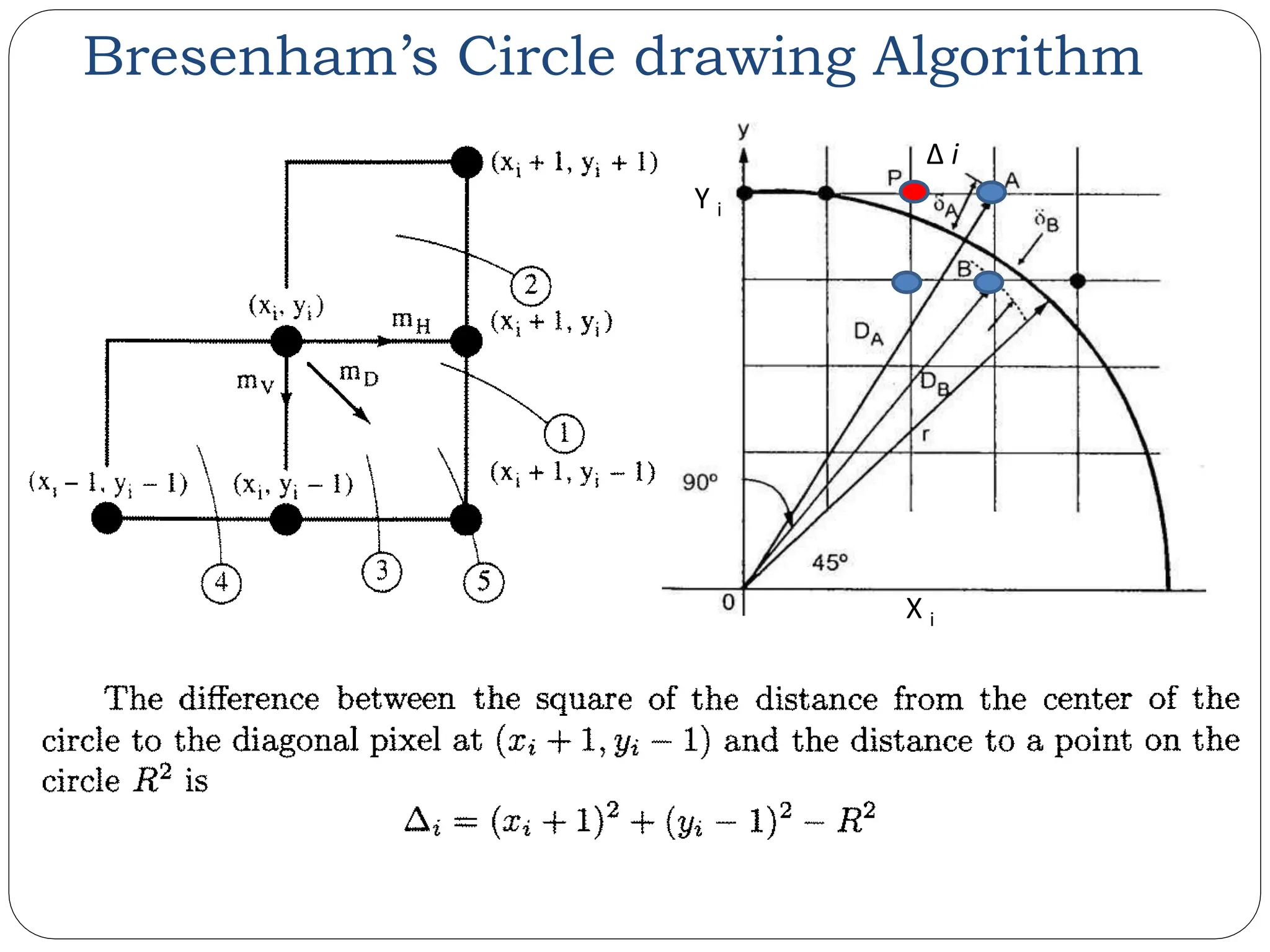
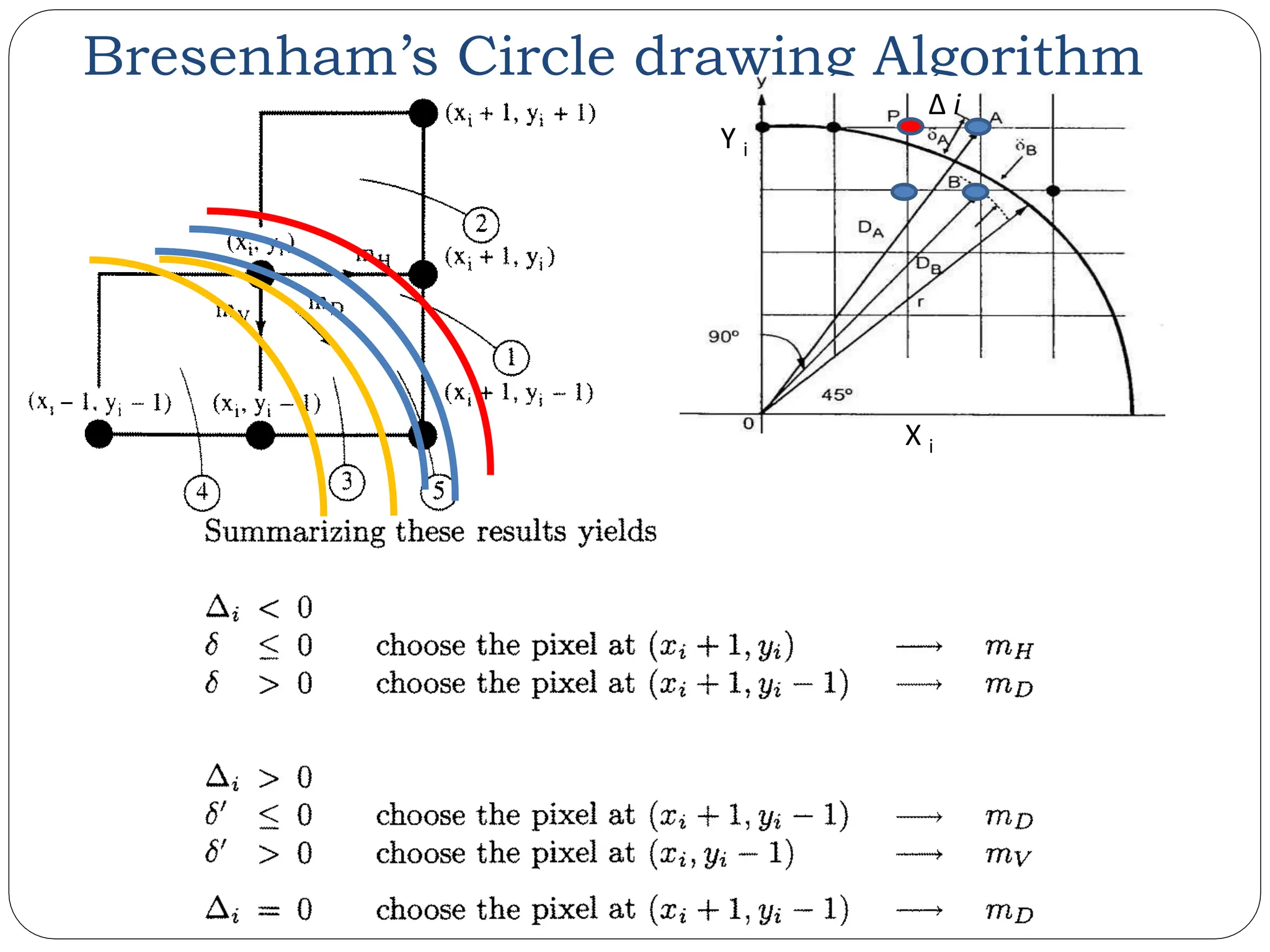
![Bresenham’s Circle drawing Algorithm Let us simplify, δA = mD - mV 𝝏𝑩 = | (𝒙𝒊 + 𝟏)𝟐 + 𝒚𝒊 − 𝟏 𝟐 - R 2 | - | ( x𝒊 2 + 𝒚𝒊 − 𝟏 𝟐 - R 2 ) | 𝜕𝐵 = | (𝒙𝒊 + 𝟏)𝟐 + 𝒚𝒊 − 𝟏 𝟐 − R 2 | - | ( (𝒙𝒊 + 𝟏)𝟐 + 𝒚𝒊 − 𝟏 𝟐 - R 2) | − 2𝒙𝒊 − 1 𝜕𝐵 = 2| ( (𝑥𝑖 + 1)2 + 𝒚𝒊 − 𝟏 𝟐 − R 2 ) | - 2𝒙𝒊 - 1 𝜕𝐵 = 𝟐Δ 𝒊 − 2𝒚𝒊 − 1 𝜕𝐵 = | (𝒙𝒊 + 𝟏)𝟐 + 𝒚𝒊 − 𝟏 𝟐 − R 2 | - | ( (𝑥𝑖 2 + 𝟐 𝒙 + 𝟏 + 𝑦𝑖 − 1 2 - R 2) | − 2x𝒊 − 1 𝜕𝐵 = 𝟐 ( 𝜟 𝒊 − 𝒙𝒊 ) - 1 ---------[ IV ] 𝜕𝐵 = | (𝒙𝒊 + 𝟏)𝟐 + 𝒚𝒊 − 𝟏 𝟐 − R 2 | - | ( (𝑥𝑖 2 + (𝟐 𝒙 + 𝟏) + 𝑦𝑖 − 1 2 - R 2) | − (2x𝒊+1 Δ 𝒊 = ( (𝒙𝒊 + 𝟏)𝟐 + 𝒚𝒊 − 𝟏 𝟐 − R 2 )](https://image.slidesharecdn.com/unit-2rasterscangraphics-240510102813-03304cf8/75/Study-on-Fundamentals-of-Raster-Scan-Graphics-35-2048.jpg)
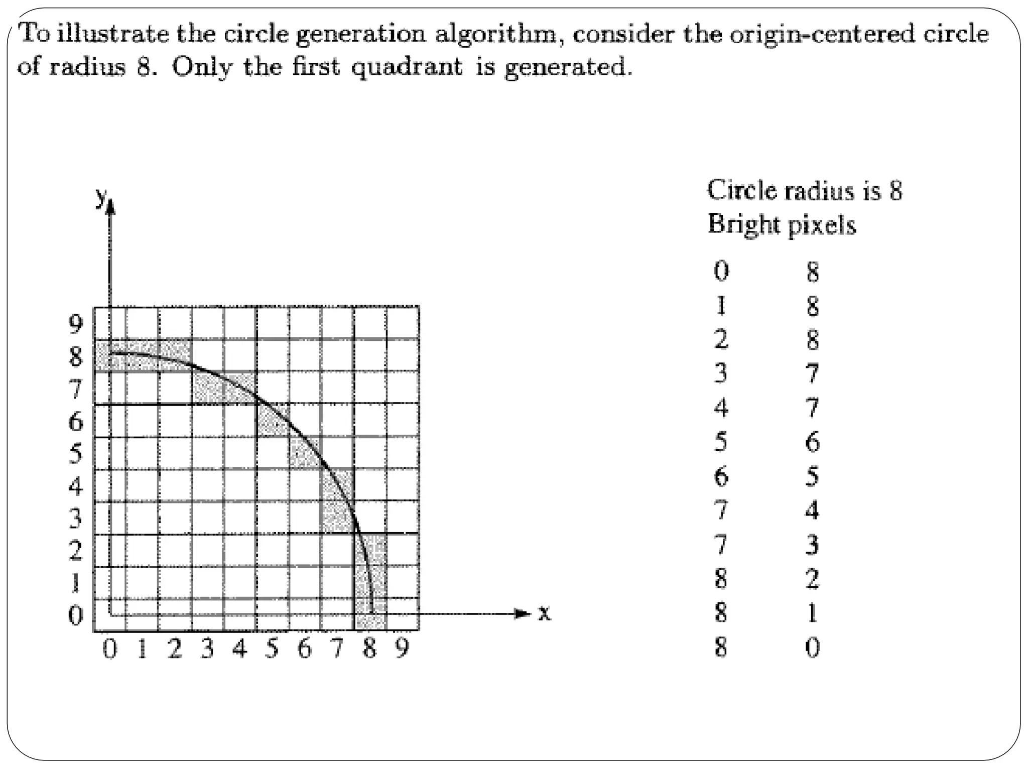
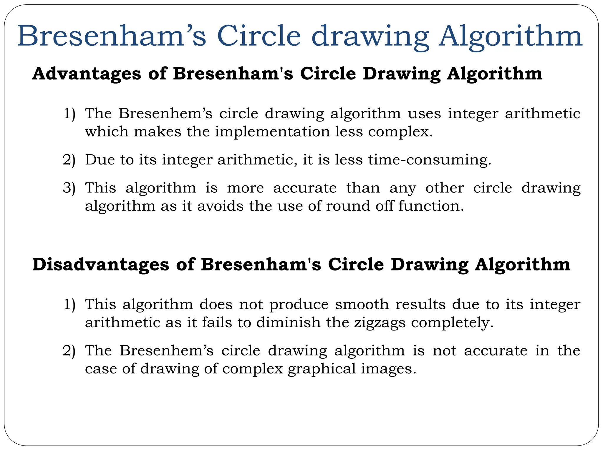


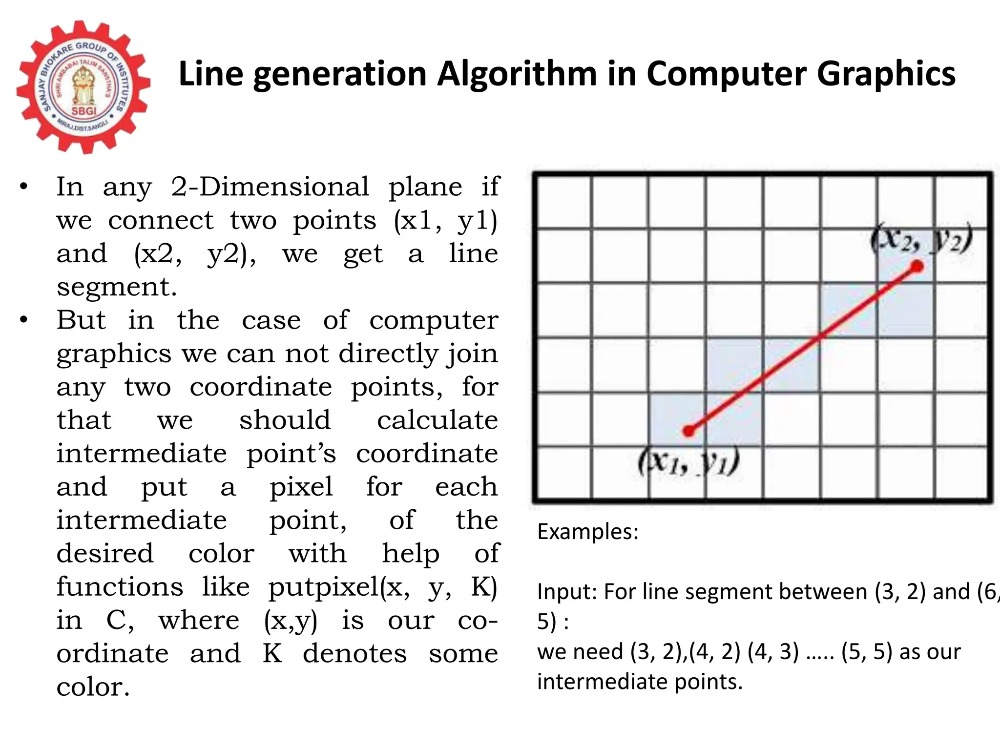
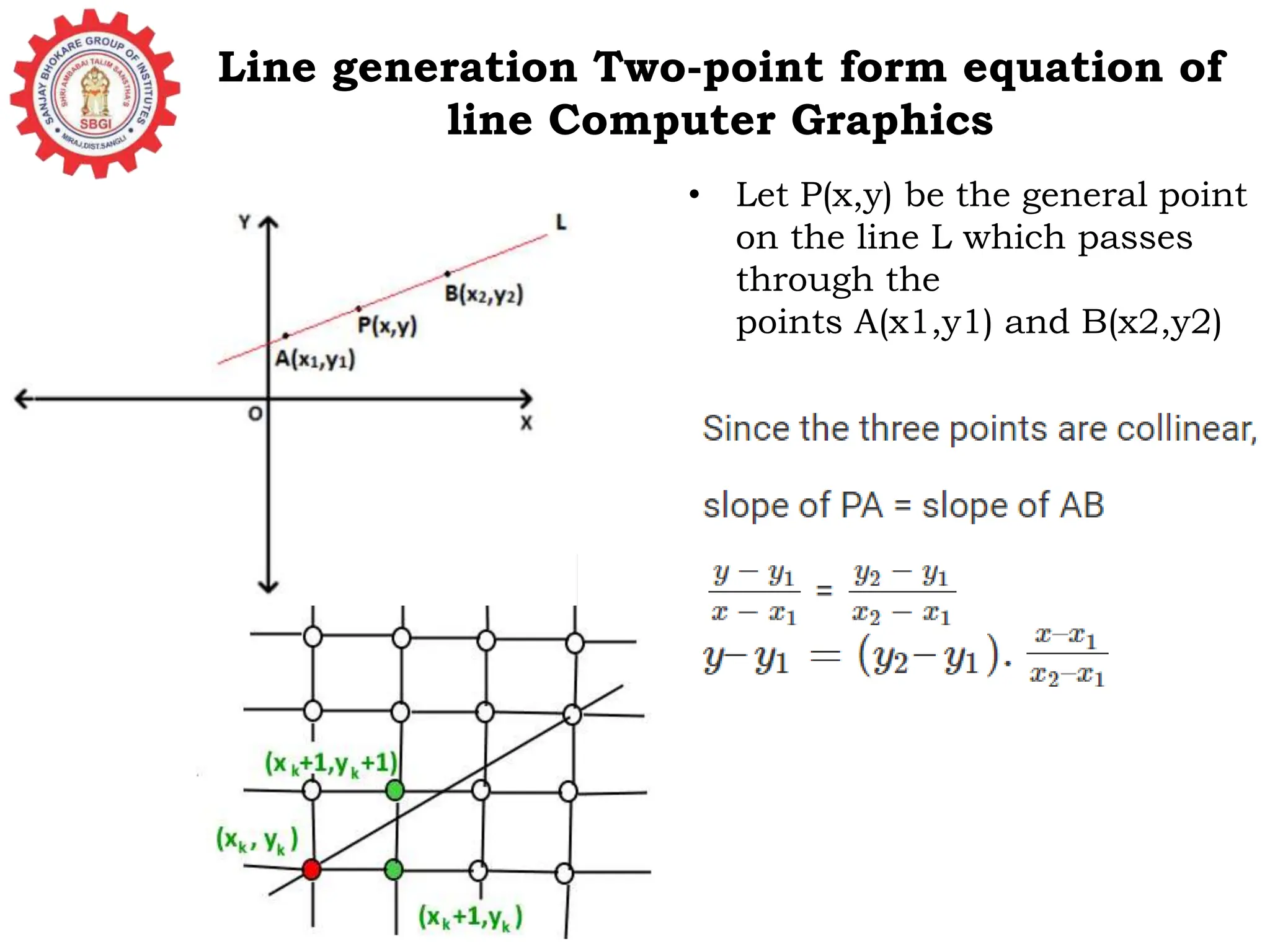
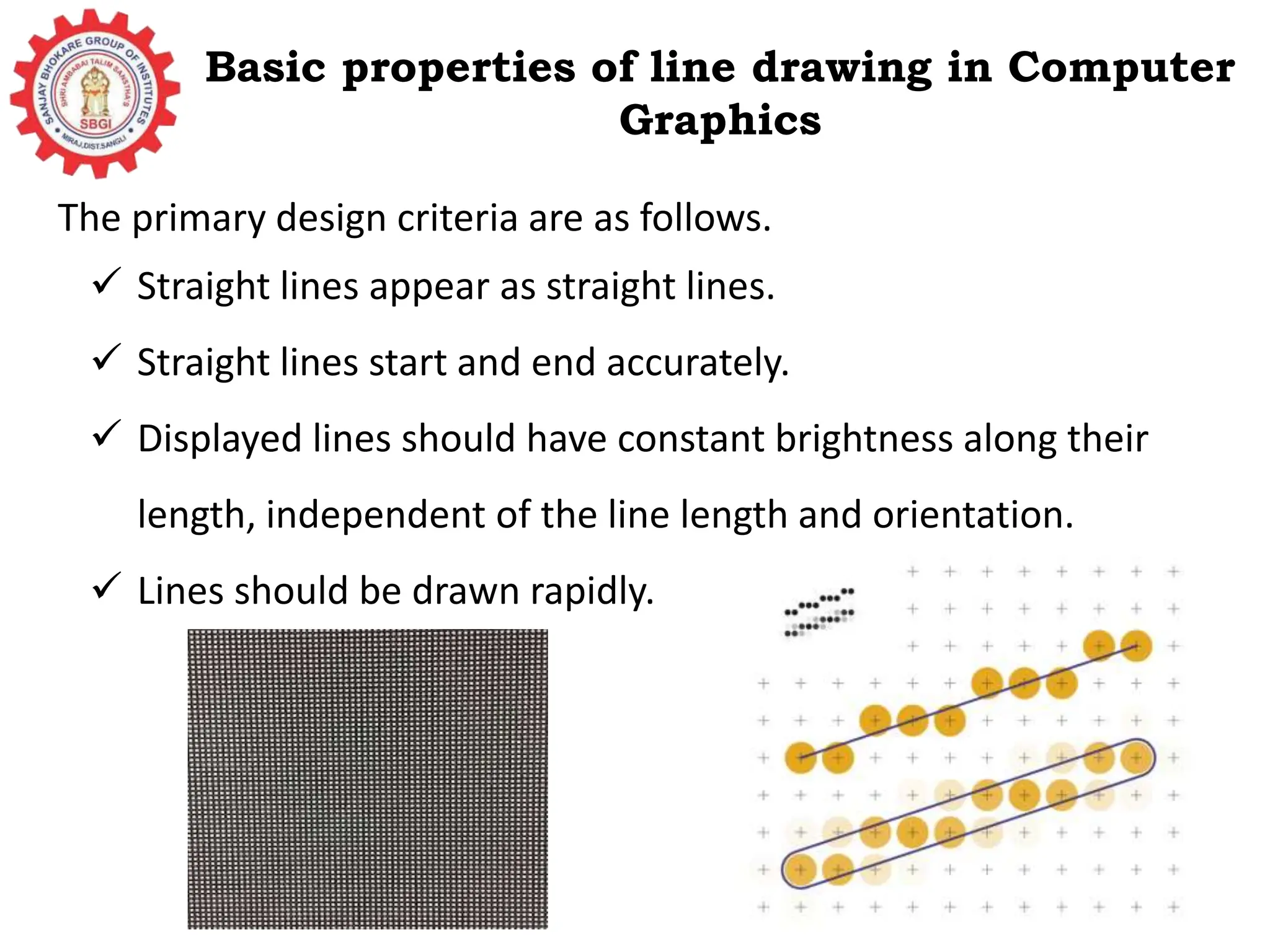
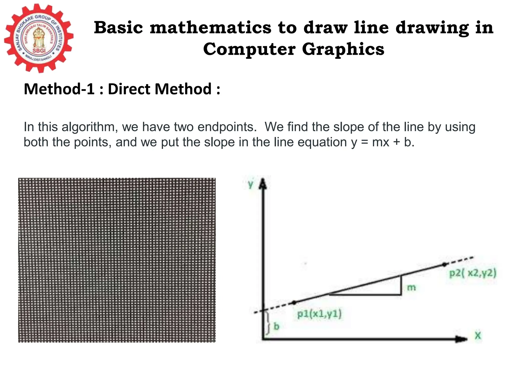
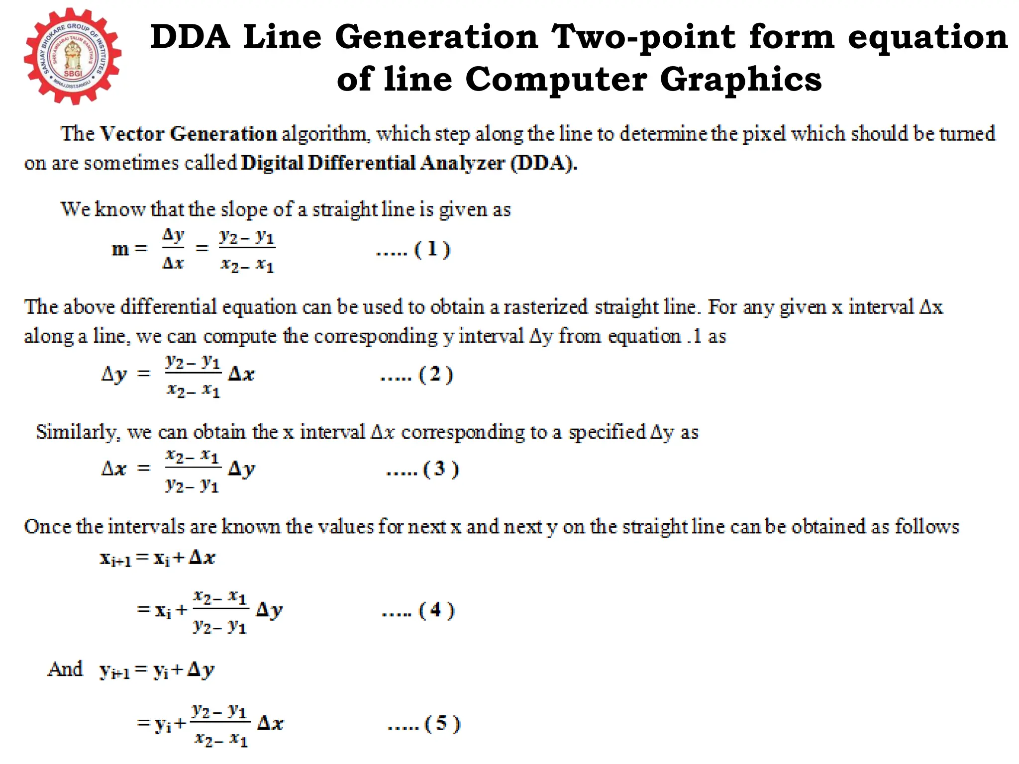
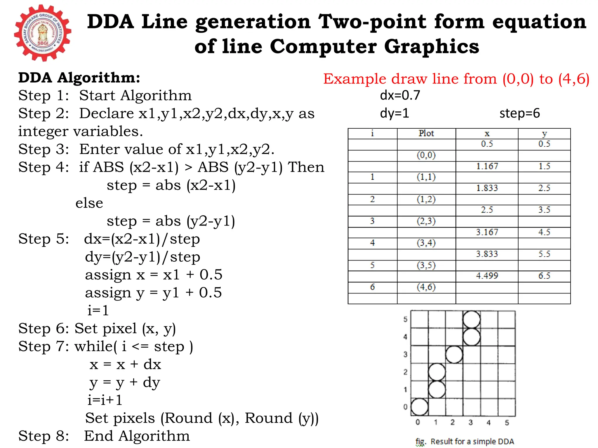
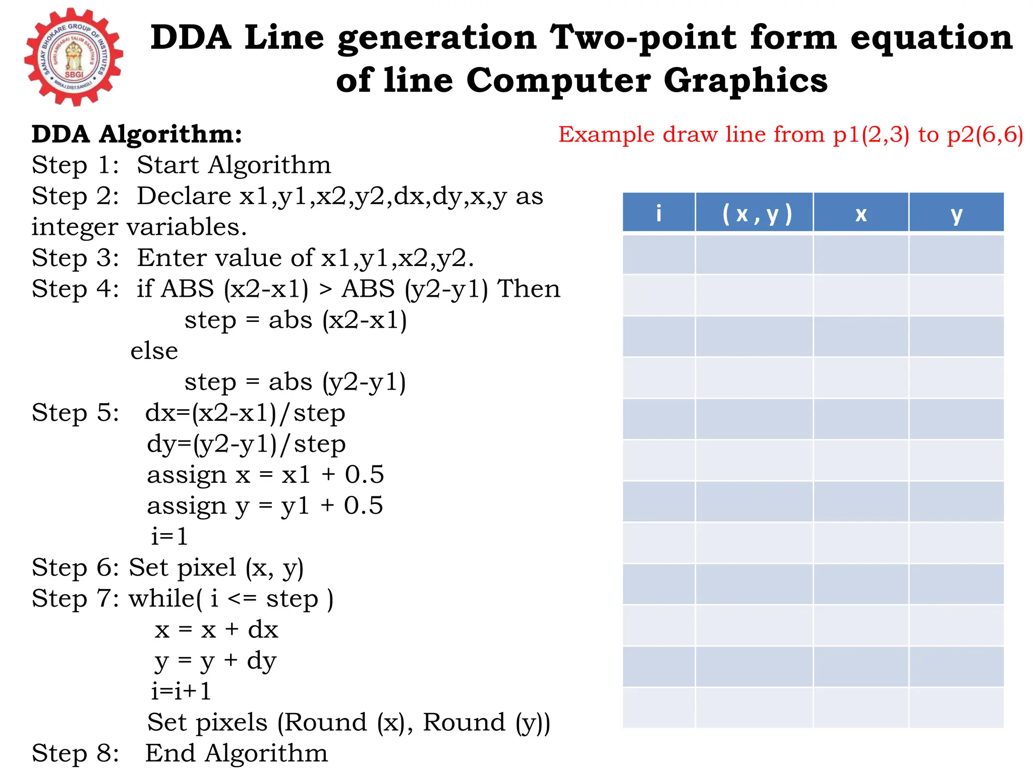
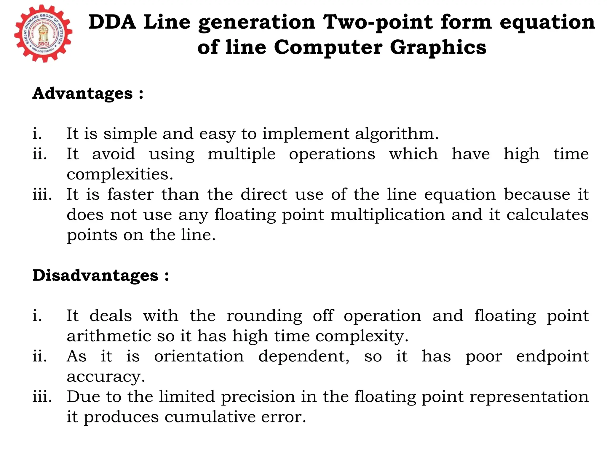
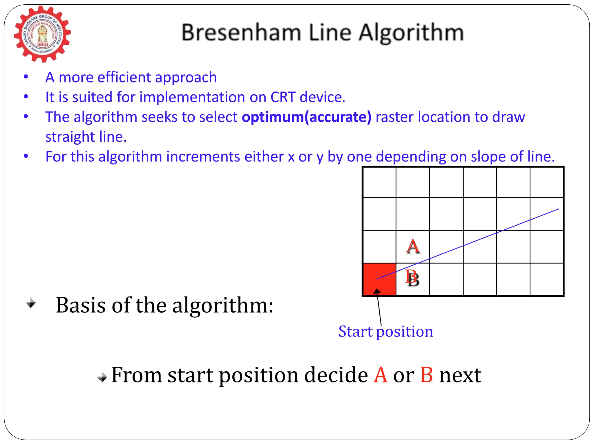
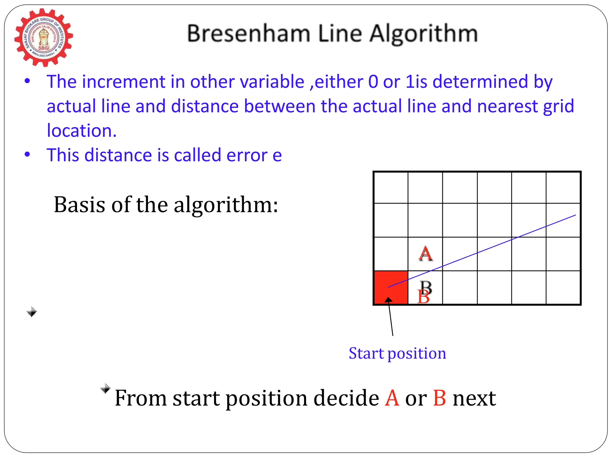
The document provides a detailed overview of line generation algorithms in computer graphics, focusing on methods like DDA and Bresenham's algorithms. It explains the mathematical principles for calculating pixel coordinates for rendering lines and circles, detailing the steps involved in these algorithms along with their advantages and disadvantages. Additionally, it discusses properties required for effective line drawing in terms of accuracy, precision, and performance.