Downloaded 86 times


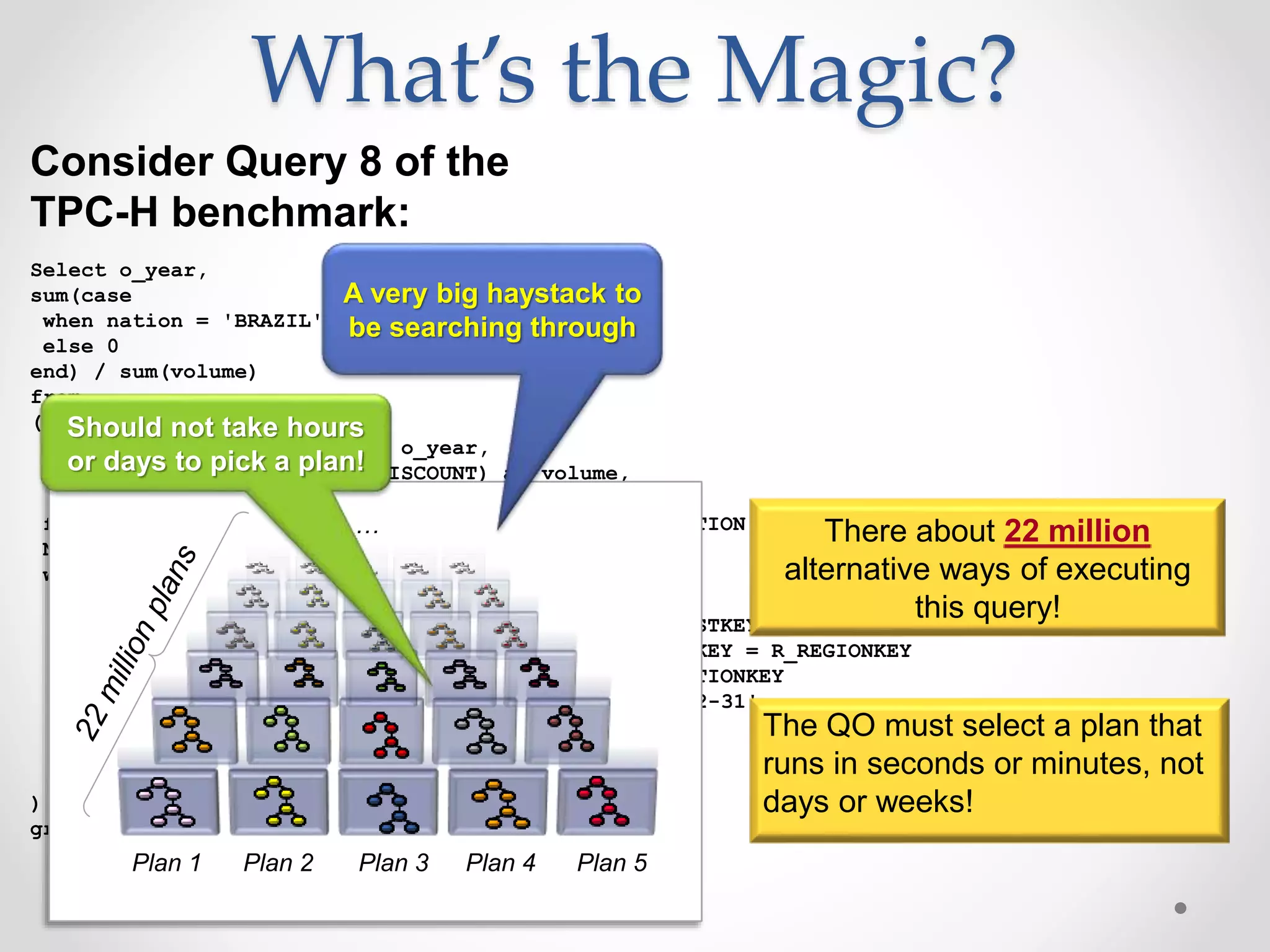
![A First Example 9 Query Execution Engine Query Optimizer Parser SELECT Average(Rating) FROM Reviews WHERE MID = 932 Reviews Date CID MID Rating … … … … Logical operator tree Avg (Rating) Select MID = 932 Reviews Query Plan #1 Avg_agg [Cnt, Sum] Scan Reviews Filter MID = 932 Avg_agg [Cnt, Sum] Index Lookup MID = 932 MID Index Reviews Query Plan #2 or](https://image.slidesharecdn.com/sqlqo-180628124507/75/SQL-Query-Optimization-Why-Is-It-So-Hard-to-Get-Right-9-2048.jpg)
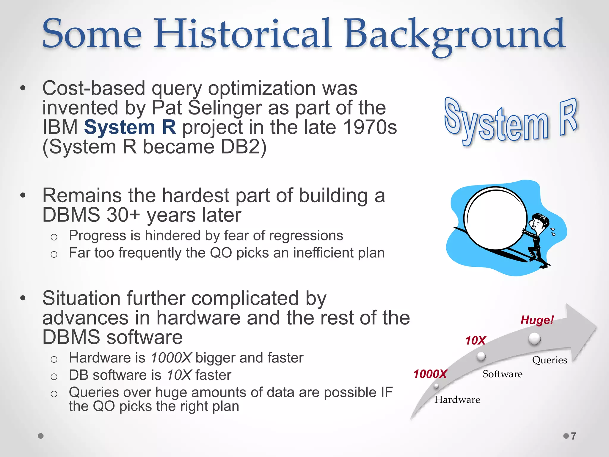
![Query Plan #1 • Plan starts by scanning the entire Reviews table o # of disk I/Os will be equal to the # of pages in the Reviews table o I/Os will be sequential. Each I/O will require about 0.1 milliseconds (0.0001 seconds) • Filter predicate “MID = 932” is applied to all rows • Only rows that satisfy the predicate are passed on to the average computation 10 Avg_agg [Cnt, Sum] Scan Reviews Filter MID = 932](https://image.slidesharecdn.com/sqlqo-180628124507/75/SQL-Query-Optimization-Why-Is-It-So-Hard-to-Get-Right-10-2048.jpg)
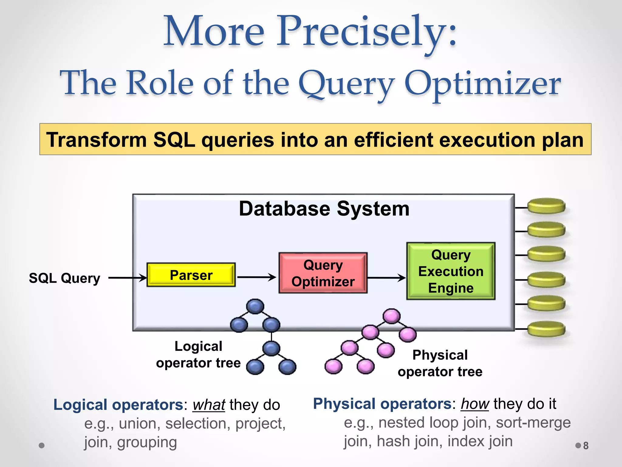
![Query Plan #2 • MID index is used to retrieve only those rows whose MID field (attribute) is equal to 932 o Since index is not “clustered”, about one disk I/O will be performed for each row o Each disk I/O will require a random seek and will take about 3 milliseconds (ms) • Retrieved rows will be passed to the average computation 11 Avg_agg [Cnt, Sum] Index Lookup MID = 932 MID Index Reviews](https://image.slidesharecdn.com/sqlqo-180628124507/75/SQL-Query-Optimization-Why-Is-It-So-Hard-to-Get-Right-11-2048.jpg)
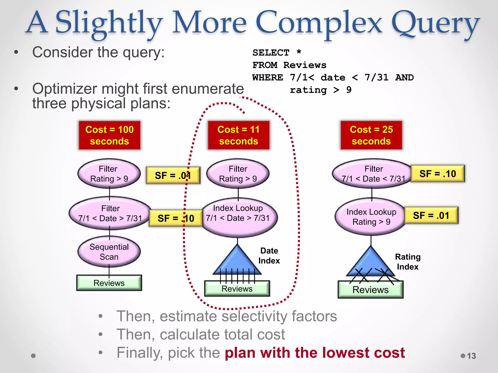
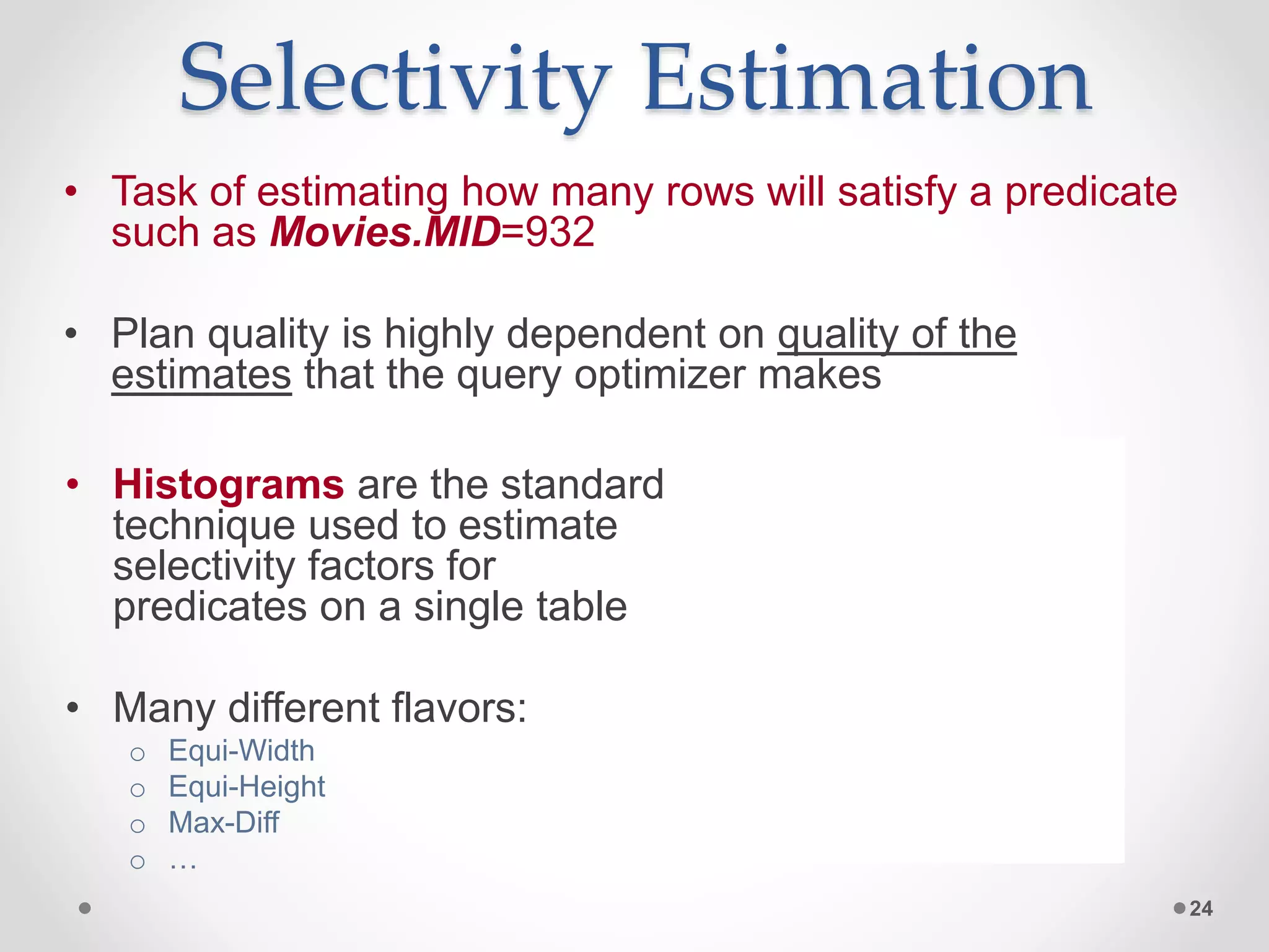
![Which Plan Will be Faster? • Query optimizer must pick between the two plans by estimating the cost of each • To estimate the cost of a plan, the QO must: o Estimate the selectivity of the predicate MID=932 o Calculate the cost of both plans in terms of CPU time and I/O time • The QO uses statistics about each table to make these estimates • The “best” plan depends on how many reviews there are for movie with MID = 932 12 Query Plan #1 Avg_agg [Cnt, Sum] Scan Reviews Filter MID = 932 Avg_agg [Cnt, Sum] Index Lookup MID = 932 MID Index Reviews Query Plan #2 Vs. How many reviews for the movie with MID = 932 will there be? Best Query Plan or? ??](https://image.slidesharecdn.com/sqlqo-180628124507/75/SQL-Query-Optimization-Why-Is-It-So-Hard-to-Get-Right-12-2048.jpg)
![Equivalence Rules (cont.) 16 Project [CID, Name] Customers Project [Name] Project operators cascade Project [Name] Customers Select operator distributes over joins Select Join Customers Reviews Select Join Customers Reviews](https://image.slidesharecdn.com/sqlqo-180628124507/75/SQL-Query-Optimization-Why-Is-It-So-Hard-to-Get-Right-16-2048.jpg)

![An Example • Query: o SELECT Avg(Rating) FROM Reviews WHERE MID = 932 • Two physical query plans: 32 Reviews Date CID MID Rating Plan #1 Avg_agg [Cnt, Sum] Sequential Scan Reviews Filter MID = 932 Avg_agg [Cnt, Sum] Index Lookup MID = 932 MID Index Reviews Plan #2 Which plan is cheaper ???](https://image.slidesharecdn.com/sqlqo-180628124507/75/SQL-Query-Optimization-Why-Is-It-So-Hard-to-Get-Right-32-2048.jpg)
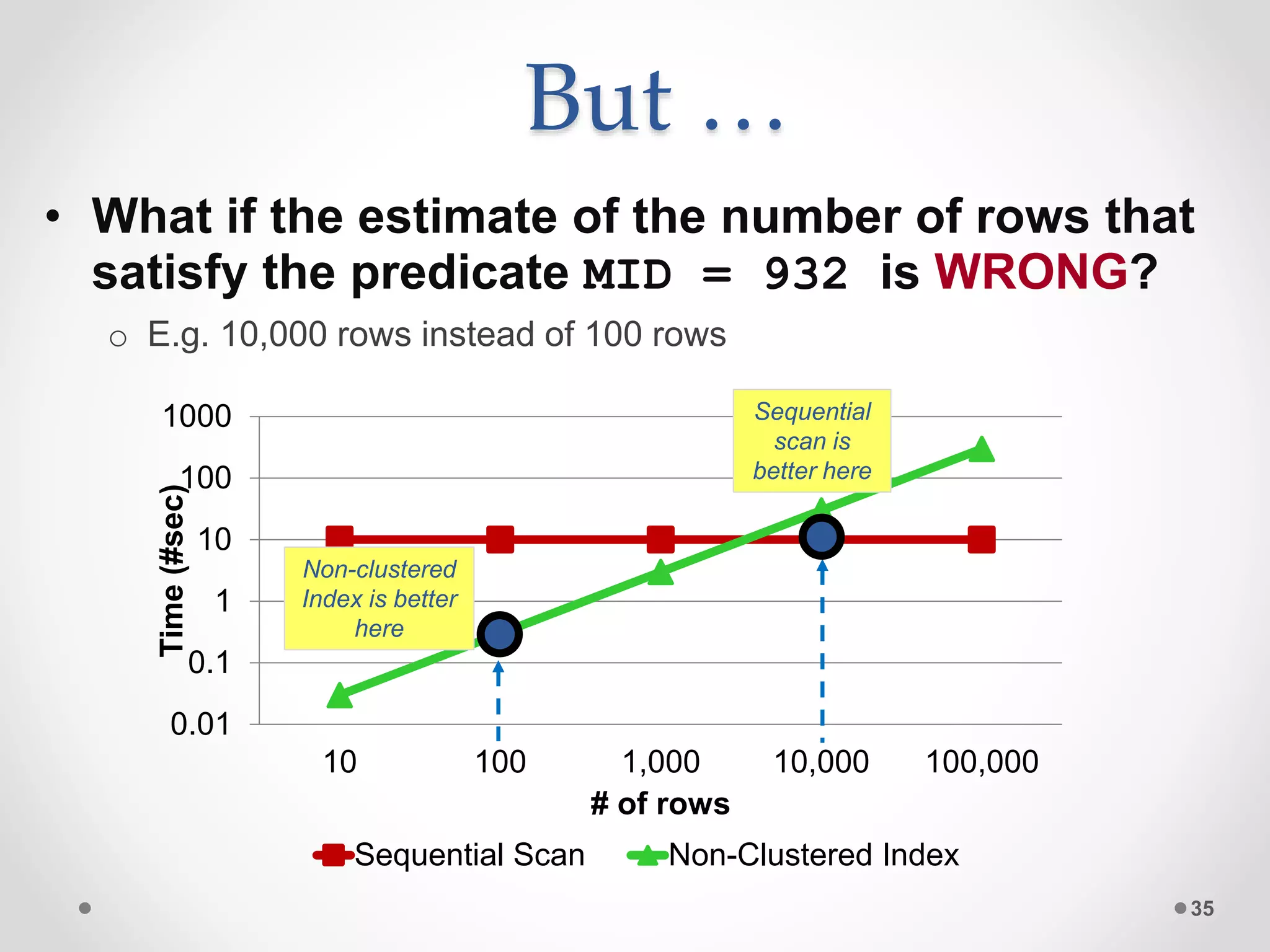
![Plan #1 33 Avg_agg [Cnt, Sum] Scan Reviews Filter MID = 932 • Filter is applied to 10M rows • The optimizer estimates that 100 rows will satisfy the predicate • Table is 100K pages with 100 rows/page • Sorted on date • Average computation is applied to 100 rows • Reviews is scanned sequentially at 100 MB/second • I/O time of scan is 8 seconds • At 0.1 microseconds/row, filter consumes 1 second of CPU time • At 0.1 microseconds/row, avg consumes .00001 seconds of CPU time Optimizer estimates total execution time of 9 seconds](https://image.slidesharecdn.com/sqlqo-180628124507/75/SQL-Query-Optimization-Why-Is-It-So-Hard-to-Get-Right-33-2048.jpg)
![Plan #2 34 Avg_agg [Cnt, Sum] Index Lookup MID = 932 MID Index Reviews • 100 rows are estimated to satisfy the predicate • Average computation is applied to 100 rows • At 0.1 microseconds/row, average consumes .00001 seconds of CPU time • 100 rows are retrieved using the MID index • Since table is sorted on date field (and not MID field), each I/O requires a random disk I/O – about .003 seconds per disk I/O • I/O time will be .3 seconds Optimizer estimates total execution time of 0.3 seconds The estimate for Plan #1 was 9 seconds, so Plan #2 is clearly the better choice](https://image.slidesharecdn.com/sqlqo-180628124507/75/SQL-Query-Optimization-Why-Is-It-So-Hard-to-Get-Right-34-2048.jpg)


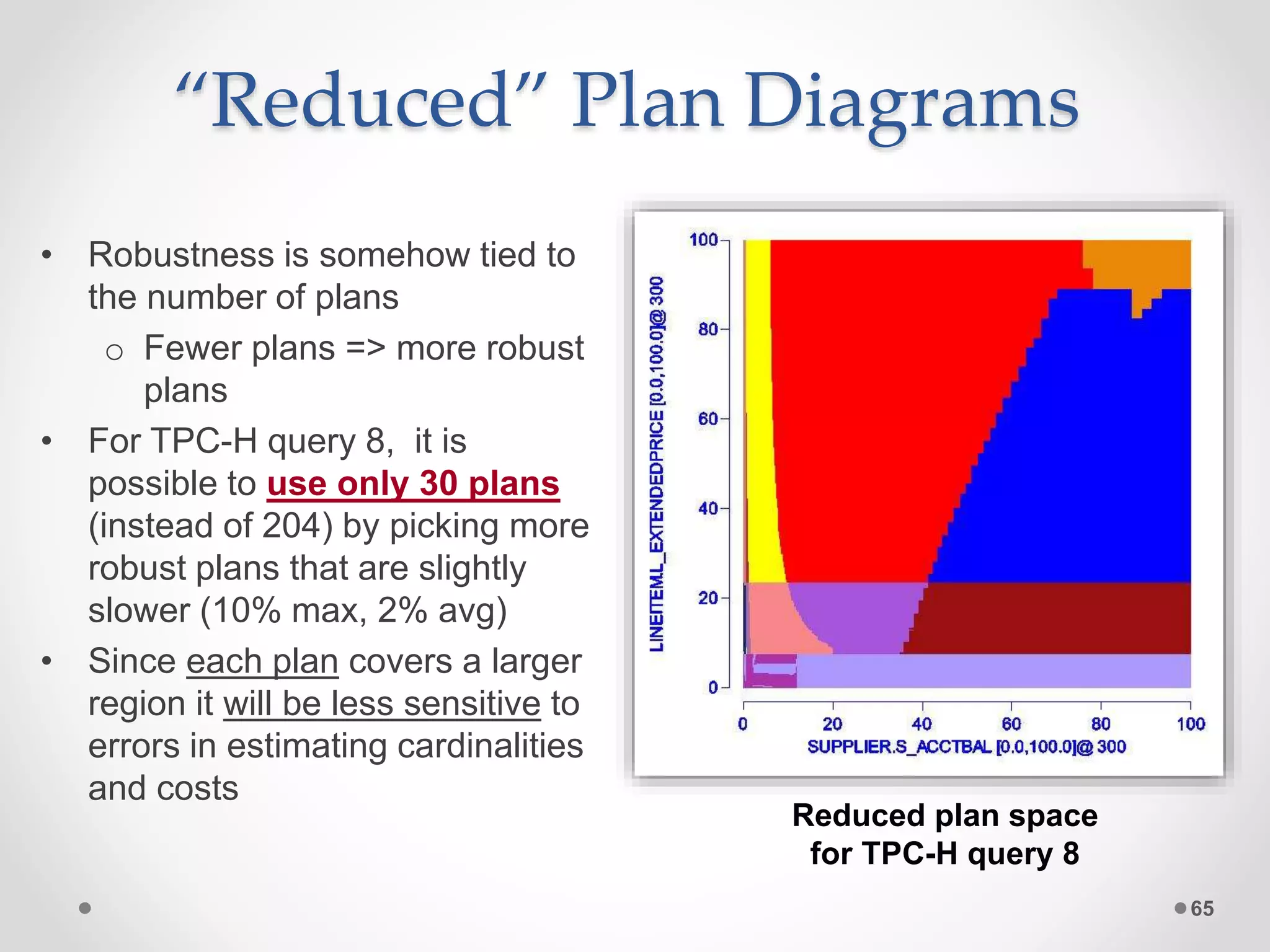
![Resulting Plan Space • SQL Server 2008 R2 • A total of 90,000 queries o 300 different values for both L_ExtendedPrice and S_AcctBal • 204 different plans!! o Each distinct plan is assigned a unique color • Zooming in to the [0,20:0,40] region: 63 Key takeaway: If plan choice is so sensitive to the constants used, it will undoubtedly be sensitive to errors in statistics and cardinality estimates Intuitively, this seems very bad!](https://image.slidesharecdn.com/sqlqo-180628124507/75/SQL-Query-Optimization-Why-Is-It-So-Hard-to-Get-Right-63-2048.jpg)
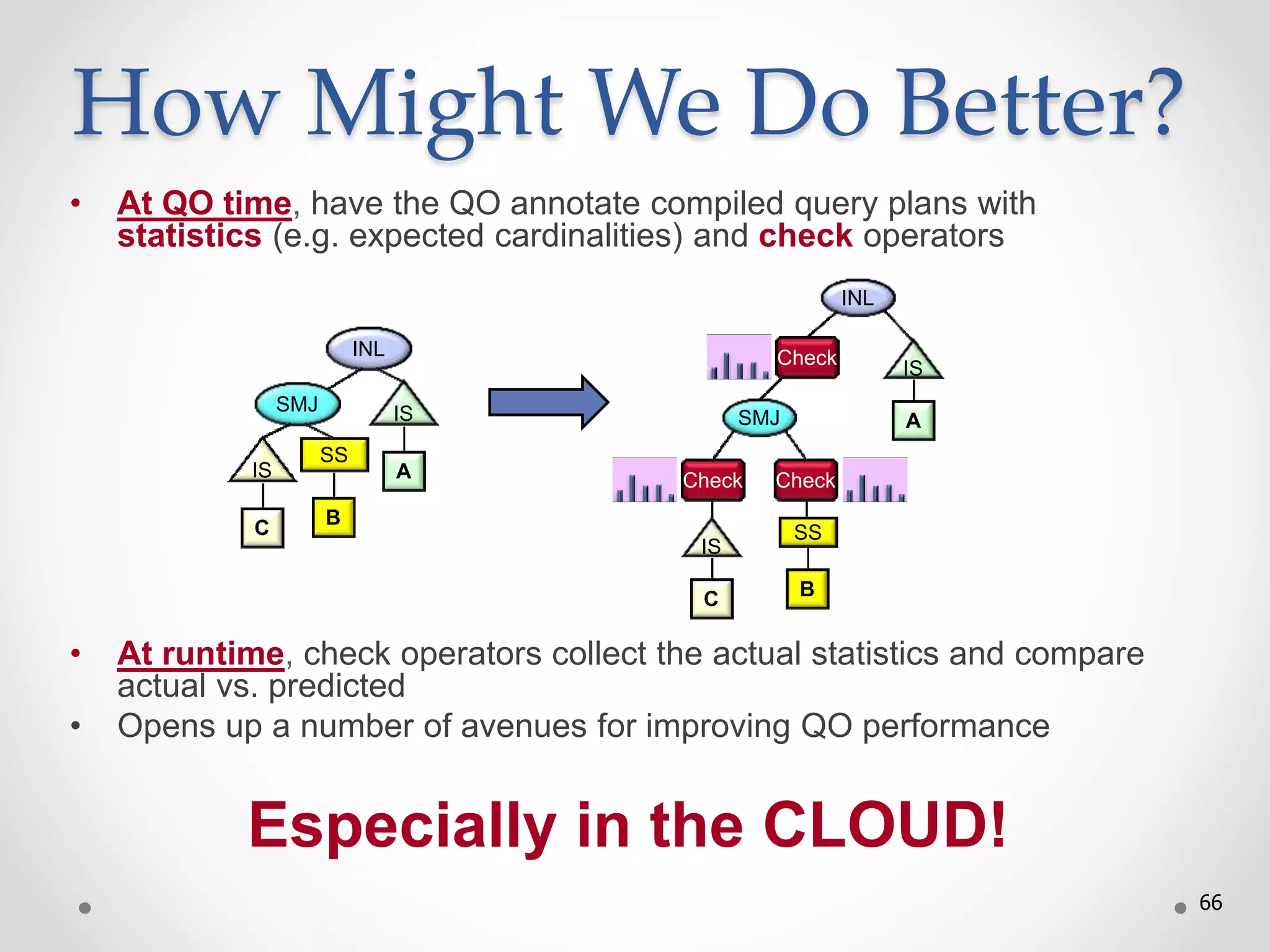


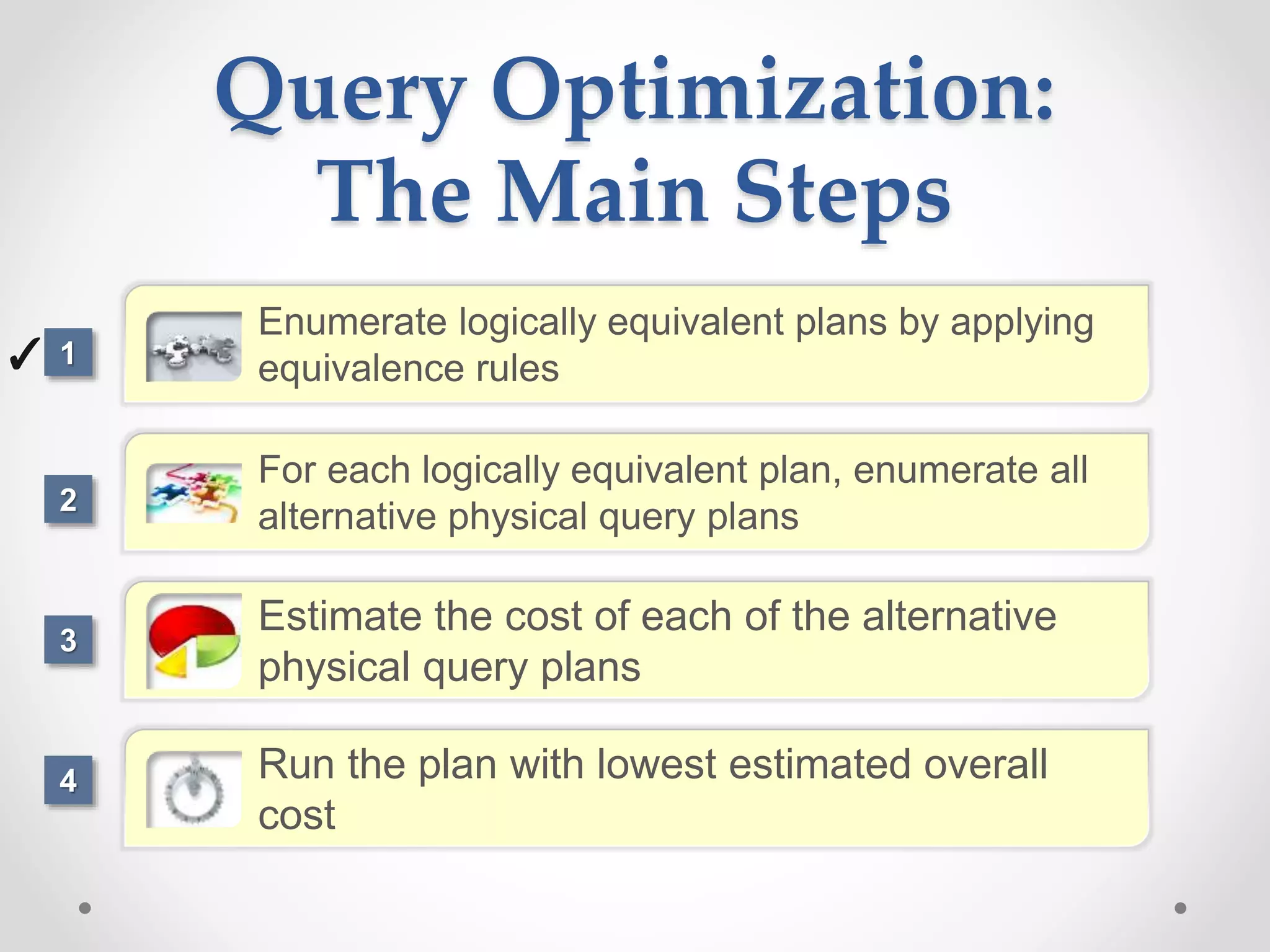
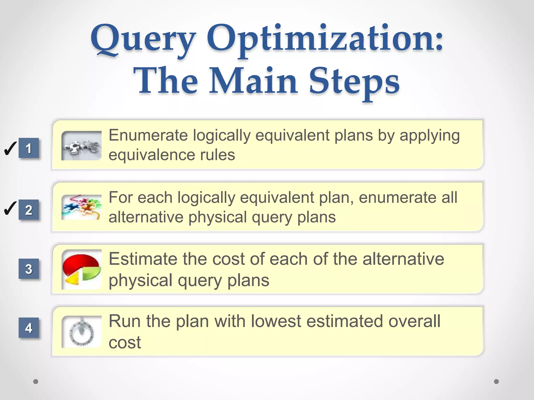
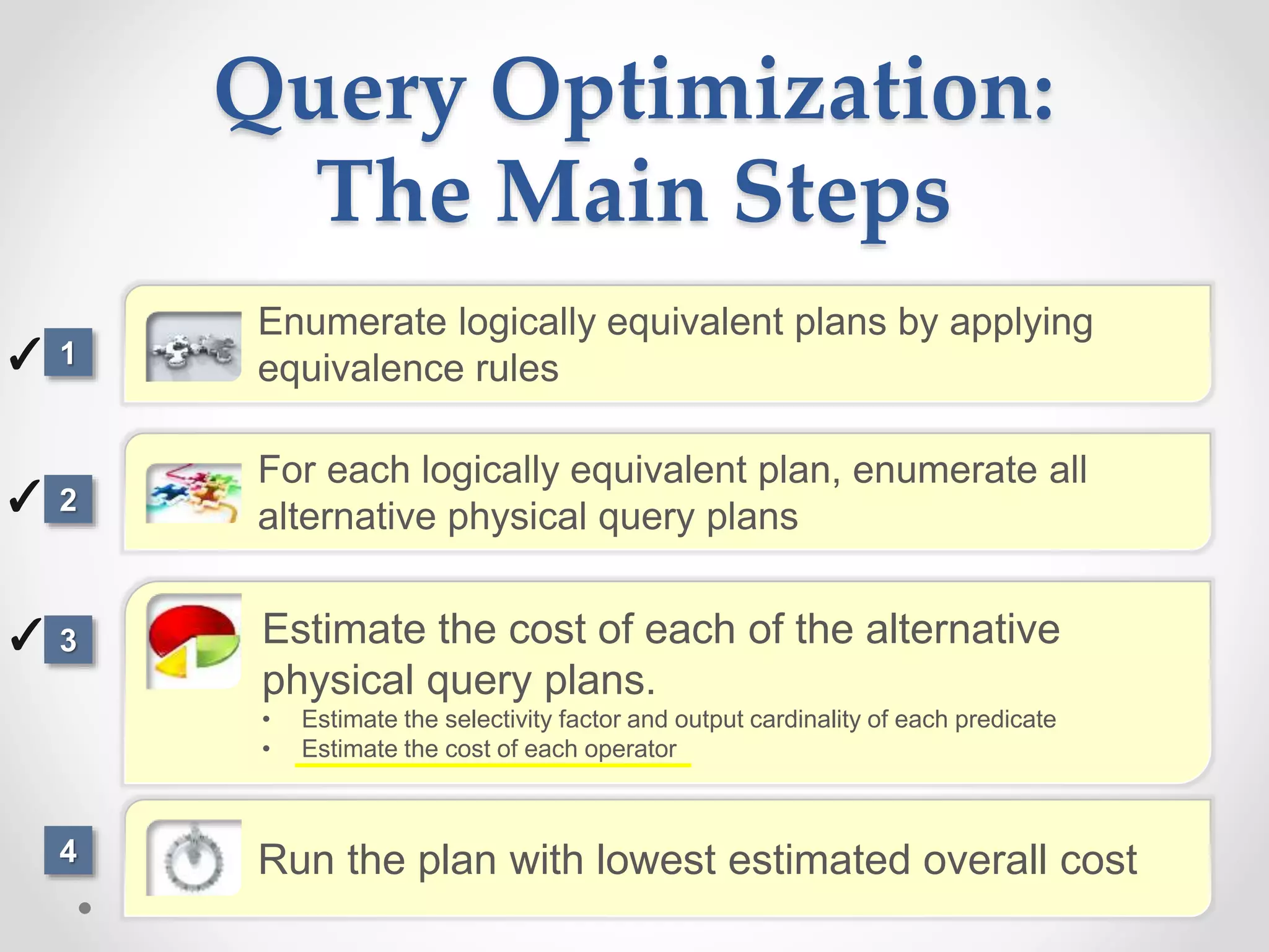
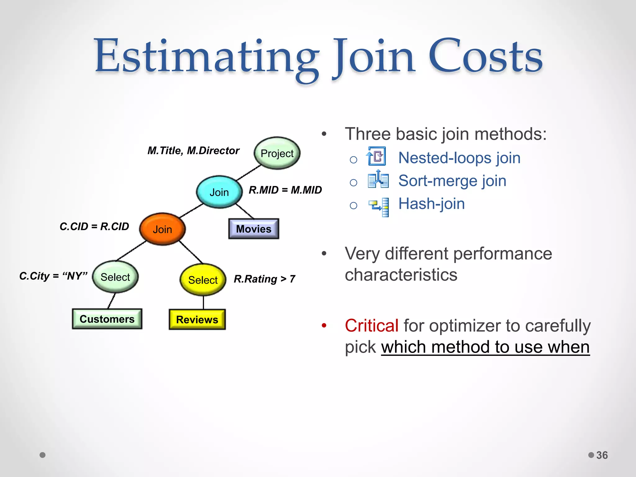
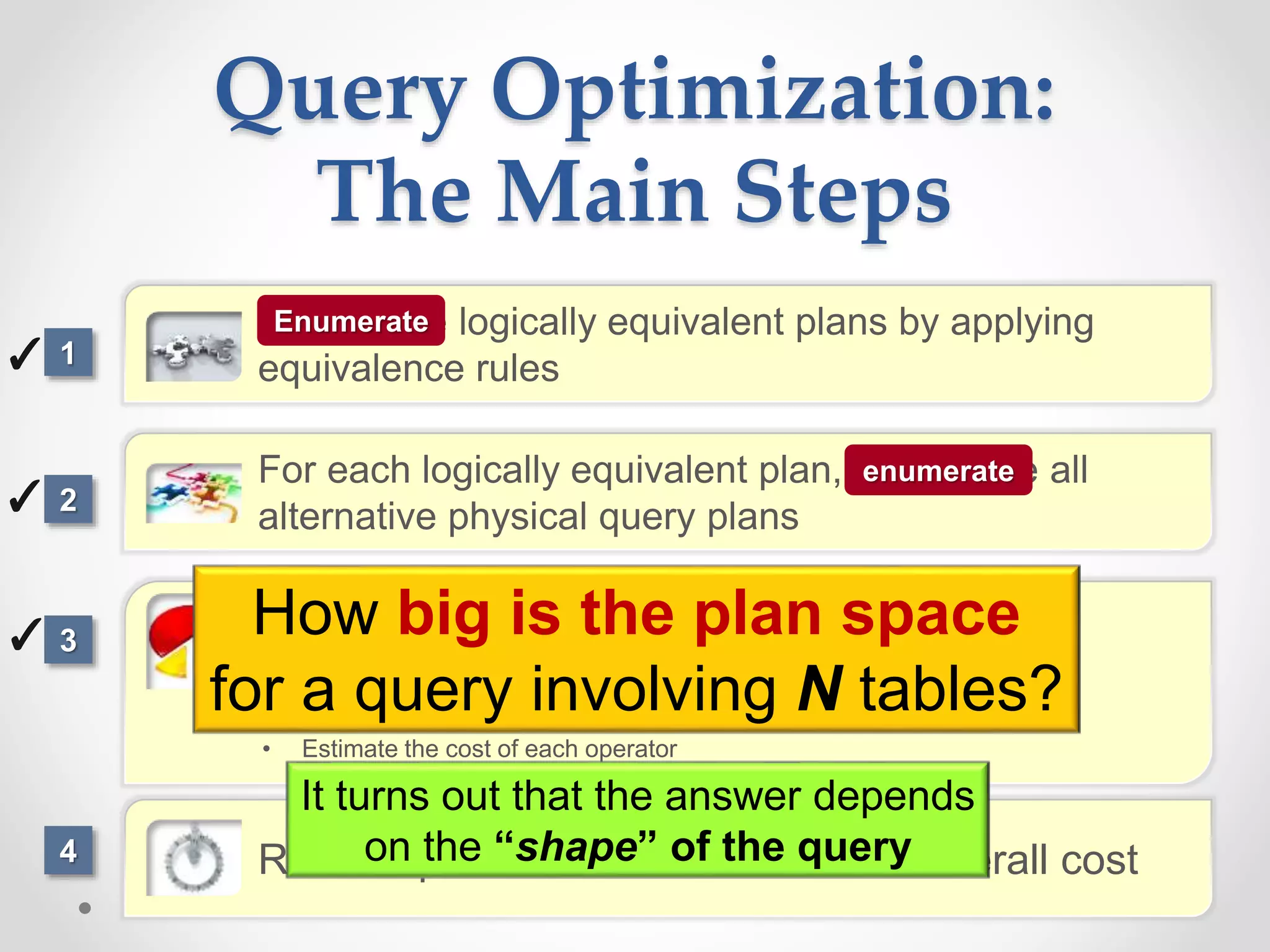
The query optimizer's role is to transform SQL queries into efficient execution plans by: 1) Enumerating logically equivalent query plans through equivalence rules. 2) Enumerating physical execution plans for each logical plan. 3) Estimating the costs of each physical plan by estimating predicate selectivities and operator costs. 4) Selecting the physical plan with the lowest estimated cost to run the query.