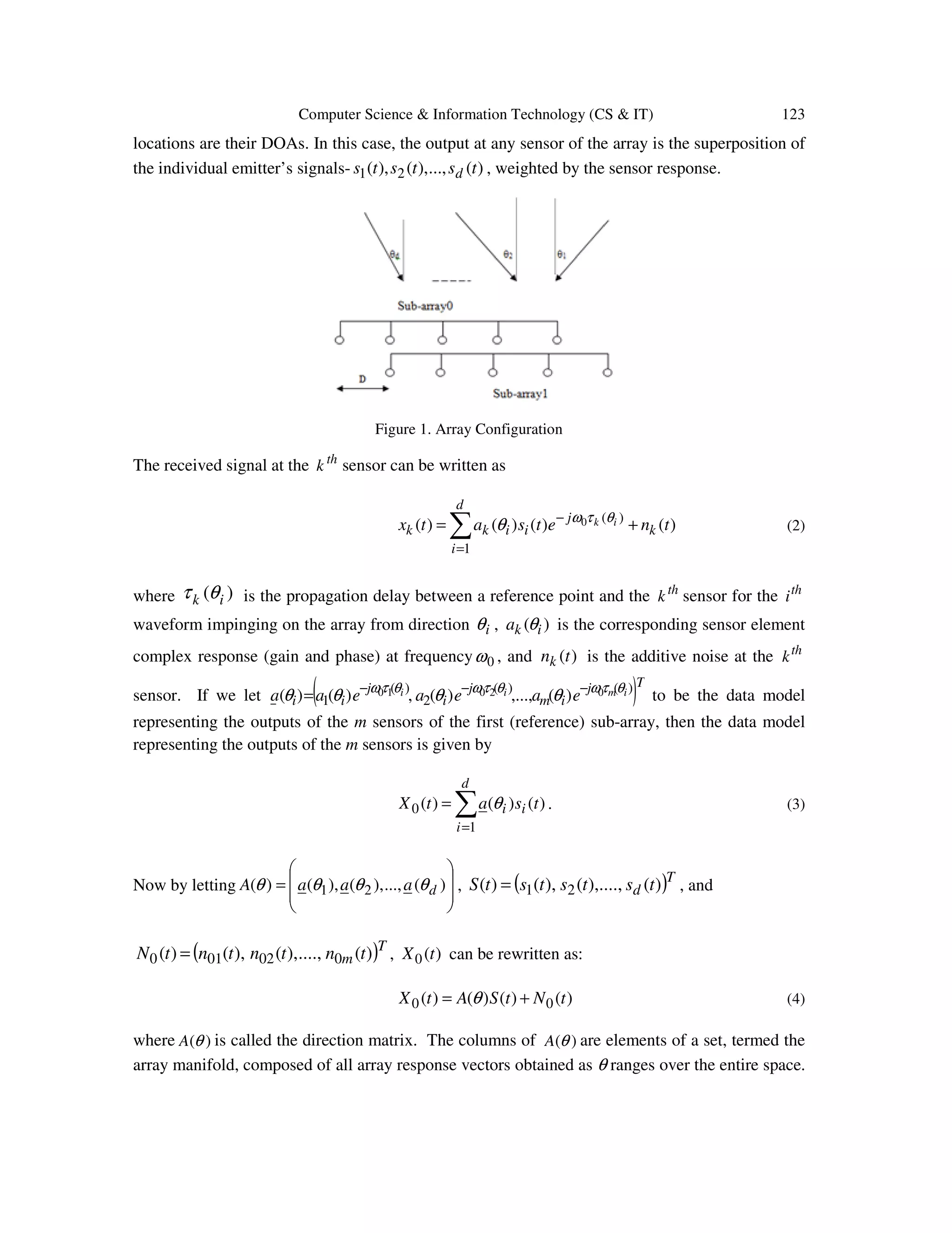
The document presents a method for resolving cyclic ambiguities and enhancing the accuracy of direction-of-arrival (DOA) estimation using a modified ESPRIT algorithm that incorporates array rotation and multiple signal sampling positions. The approach aims to tackle the performance limitations of conventional methods caused by measurement errors and angle of incidence, ultimately providing more reliable DOA estimates, verified through simulation results. It discusses the impact of parameters such as signal-to-noise ratio and the number of snapshots on the algorithm's effectiveness.
![Jae-Kwang Lee et al. (Eds) : CCSEA, AIFU, DKMP, CLOUD, EMSA, SEA, SIPRO - 2017 pp. 121– 138, 2017. © CS & IT-CSCP 2017 DOI : 10.5121/csit.2017.70212 RESOLVING CYCLIC AMBIGUITIES AND INCREASING ACCURACY AND RESOLUTION IN DOA ESTIMATION USING ARRAY ROTATION AbdelhamidDjouadi1 and NebojsaI. Jaksic2 1 Nokia, 4575 Rings Rd, Dublin, Ohio, USA 2 Colorado State University - Pueblo, 2200 Bonforte Blvd., Pueblo, Colorado, USA ABSTRACT A method to resolve cyclic ambiguities and increase the accuracy and the resolution in the direction-of-arrival (DOA) estimation using the Estimation of Signal Parameters via Rotational Invariance Technique (ESPRIT)algorithm is proposed. It is based on rotating the array and sampling the received signal at multiple positions. Using this approach, the gain in accuracy and resolution is addressed as function of the mean and variance of the DOA. Simulations results are provided as a means of verifying this analysis. KEYWORDS Direction Of Arrival (DOA) estimation, Estimation of Signal Parameters via Rotational Invariance Technique (ESPRIT), Total Least Square (TLS), Cyclic Ambiguities 1. INTRODUCTION Because of the widespread use of sensor arrays, and the continuing development of their capabilities, sensor arrays have experienced an increased range of applications. One of these applications that has been given special attention is the high resolution direction-of-arrival (DOA) estimation. This estimation is mainly based on the processing of the received signal to extract the desired parameters of DOA of plane waves upon which the sensor outputs depend. The estimation of Signal Parameters by Rotational Invariance Techniques (ESPRIT) is one of the many approaches that have been used for implementing the DOA functions[1].In essence, and for the narrowband direction-of-arrival case, ESPRIT algorithm estimates a unitary diagonal matrix Φ with diagonal elements, given by die ij i ,...1; == − µ ϕ , where d is the number of sources impinging on the array from distinct locations dθθθ ,...,, 21 , as shown in Figure 1, and where the parameters dii ,...,1; =µ , denote the phase shifts to be estimated. For a uniform linear array (ULA), it is well known that the phase shift µ is related to the angle of arrival θ by](https://image.slidesharecdn.com/csit76412-170207121240/75/RESOLVING-CYCLIC-AMBIGUITIES-AND-INCREASING-ACCURACY-AND-RESOLUTION-IN-DOA-ESTIMATION-USING-ARRAY-ROTATION-1-2048.jpg)
![122 Computer Science & Information Technology (CS & IT) λθπµ /sin2 D= (1) where λ is the wavelength of the narrow-band signal and D is the displacement vector between two sub-arrays. Various algorithms were proposed successively to improve the ESPRIT performance. However, much of the studies show that the performance of these algorithms depends only on the number of snapshots(n), the number of array sensors(m), and the signal-to-noise (SNR) of the received array signals [2 ]-[5]. Further in [6]-[8], it was shown that the performance is improved by using multi-scale method, where the short )2/( λ≤D and long baselines )2/( λ>D are, respectively, utilized to derive the coarse unambiguous and fine ambiguous estimates for each signal. The final DOA estimate in this case is determined by using the coarse estimate to disambiguate the fine estimate. This work shows that the performance of the ESPRIT algorithm is also constrained by the angle of arrivals of incidence with which the sources are impinging the array, and that the ESPRIT algorithm produces ambiguities in the estimated DOAs when the antenna element spacing on the linear array has a measurement error [9]-[10], or when the sources are impinging on the array with an angle of incidence along-side the ULA, especially for low SNR and limited number of snapshots. The purpose of this work is to show that by rotating the array and sampling the received signal at multiple positions, ambiguities in the DOA estimates are resolved and also more accurate DOA estimates are obtained. Using this approach, the gain in accuracy and resolution are addressed as function of the mean and variance of the angle of arrival errors of the sources. An analysis of simulation results is provided to verify the method described. 2. PROBLEM FORMULATION This section formulates the DOA estimation problem when using the ESPRIT algorithm and shows that its performance depends on the angle-of-arrival (incidence) with which the source is impinging the array. Also it describes the ambiguities produced in the estimated DOA results, when the antenna element spacing on a linear array is more than half a wavelength because of measurement errors, or when the sources are impinging on the array at an angle of incidence along-side the ULA. 2.1. Data Model Consider an array consisting of two sub-arrays as shown inFigure1. Each sub-array consists of m elements. The two sub-arrays are assumed to be overlapping, and separated by a displacement vector D(where Dis a fixed distance equal or smaller than half a wavelength). Assume that md < narrow-band sources impinge on the array from distinct locations dθθθ ,...,, 21 .For simplicity, it is assumed that the sources are narrow-band, no-coherent, coplanar, and that they are in the far field of the array. This assumption allows modeling the propagation delays between sensor elements as simple phase shifts, and thus the only parameters that characterize the sources](https://image.slidesharecdn.com/csit76412-170207121240/75/RESOLVING-CYCLIC-AMBIGUITIES-AND-INCREASING-ACCURACY-AND-RESOLUTION-IN-DOA-ESTIMATION-USING-ARRAY-ROTATION-2-2048.jpg)
![Computer Science & Information Technology (CS & IT) 125 where sΛ is a diagonal matrix with mdd 2121 ...... λλλλλ ==>≥≥≥ + [ ]ds eeeE ...,,, 21= is the matrix composed of the eigenvectors corresponding to the d largest eigen values that define the signal subspace, and [ ]mddn eeeE 221 ...,,, ++= is the matrix of the eigenvectors that span the complement orthogonal noisesubspace. Since the matrices = 1 0 E E Es and Φ = A A A have the same range space, then the intent of the ESPRIT algorithm is to find a nonsingular matrix T of rank d such that 1 0 E E T A A Φ = (10) By eliminating A in (10), the following expression is obtained: Ψ=Φ= − 0 1 01 ETTEE (11) where TT Φ=Ψ −1 . In general, there is no matrix Ψ that satisfies (11) exactly because 0E and 1E are equally noisy and their estimates do not span the same column subspace. The conventional ESPRIT estimates Ψ using the Least Square (LS) criterion, and thus mayyield in overall inferior results as the LS solution is known to be biased [11]. To circumvent the conventional ESPRIT algorithm drawback to some extent, the Total Least Square (TLS)-ESPRIT [11] is used instead to provide asymptotically unbiased and efficient estimates of the DOAs. The TLS estimates have been shown to be strongly consistent (convergeswith probability one to the true values). Following [11], a total least square (TLS) estimates of Ψ, given 0E and 1E ,is provided by 1 2212 − −=Ψ EETLS (12) respectively, where 12E and 22E are implicitly defined by the eigen decomposition of [ ] = = * 22 * 21 * 12 * 11 2221 1211 10* 1 * 0* | EE EE L EE EE EE E E EE def xyxy (13) where ( ) dd lllllldiagL >>>= ...,...,.,, 2121 .](https://image.slidesharecdn.com/csit76412-170207121240/75/RESOLVING-CYCLIC-AMBIGUITIES-AND-INCREASING-ACCURACY-AND-RESOLUTION-IN-DOA-ESTIMATION-USING-ARRAY-ROTATION-5-2048.jpg)
![126 Computer Science & Information Technology (CS & IT) In practical situations where only a finite number of noisy measurements are available, we have only an estimates of TLSΨ of Ψ. In this case, the eigenvalues of TLSΨ , denoted by dii ,...,1, =φ ) , give estimates of the DOAs as: )2/(sin 1 Dii πµλθ )) − = , i=1,…,d. (14) where )arg( ii φµ )) = . 2.2. ESPRIT Performance As mentioned earlier, the TLS-ESPRIT algorithm[11] leads to unbiased estimates phase shifts under the assumption that a very large number of data snapshots are available, a condition difficult to satisfy in practical situations. When the collected data snapshots are limited, the estimates do not always approach the asymptotic ones, and the realizable results vary as function of the estimation error variance of the phase shifts. In general, if we consider that the estimated phase shifts µ ) of µ are determined with an estimation error µ∆ , and with the assumption that µ∆ is a Gaussian independent process with zero mean and with variance 22 )( µσµ =∆E , then from (1), the estimates of the DOAs θ ) of θ are estimated with an error of θπ µλ θ cos2 )( D ∆ =∆ (15) Thus, θ∆ is also Gaussian with zero mean and variance θπ σλ θ µ 222 22 2 cos4 )( D E =∆ (16) One can clearly see that, as the absolute value of incidence angleθ increases, the variance of the error θ∆ will also increase. For instance, consider the case of only one source impinging on the array with 1θ corresponding to a phase shift 1µ . If this same source is impinging on the array with 2θ , it will correspond to a phase shift 2µ . With the assumption that 12 θθ > , and since uu σσσ µ == 21 , the forms of the Gaussian probability density functions of the estimated phase shifts with means 1µ and 2µ are shown in Figure 2. Likewise the Gaussian probability density functions of the corresponding estimated DOAs with mean 1θ , and 2θ , are shown in Figure 3. If we choose the intervals µβ σµ 2/1 z± and µβ σµ 2/2 z± ,where 2/βz is the z value that locates an area of )2/1( β− in the upper tail of a normal distribution, then we are certain that these intervals will contain estimates of 1µ and 2µ with a probability equal to )1( β− or a confidence level %100)1( β−=ℑ . However, we point out that while maintaining a constant confidence interval](https://image.slidesharecdn.com/csit76412-170207121240/75/RESOLVING-CYCLIC-AMBIGUITIES-AND-INCREASING-ACCURACY-AND-RESOLUTION-IN-DOA-ESTIMATION-USING-ARRAY-ROTATION-6-2048.jpg)
![Computer Science & Information Technology (CS & IT) 127 for the estimates of the phase shifts, the confidence interval of the estimates of the DOAs will increase with the angle of incidence. This is depicted in Figure 3, where the confidence interval for the estimates of 2θ is clearly wider than the confidence of the estimates of 1θ since the error of the estimates of 2θ has larger sample variance than the error of the estimates of 1θ . Figure2. Probability Density Functions of the Phase Shifts Figure 3. Probability Density Functions for the DOAs It is obvious that (16) cannot be made arbitrary small, especially for angles of incidence along- side the ULA, without putting a constraint on µσ . Maintaining a good accuracy of the estimated DOA simplies having a very small µσ . This means a higher SNR and/or an increase of the number of snapshots n. For instance, this is clearly shown for the one source case [3], where the phase shift estimation error, the SNR, and the number nof snapshots are related by = nmSNR 2 2 11 µσ . (17)](https://image.slidesharecdn.com/csit76412-170207121240/75/RESOLVING-CYCLIC-AMBIGUITIES-AND-INCREASING-ACCURACY-AND-RESOLUTION-IN-DOA-ESTIMATION-USING-ARRAY-ROTATION-7-2048.jpg)
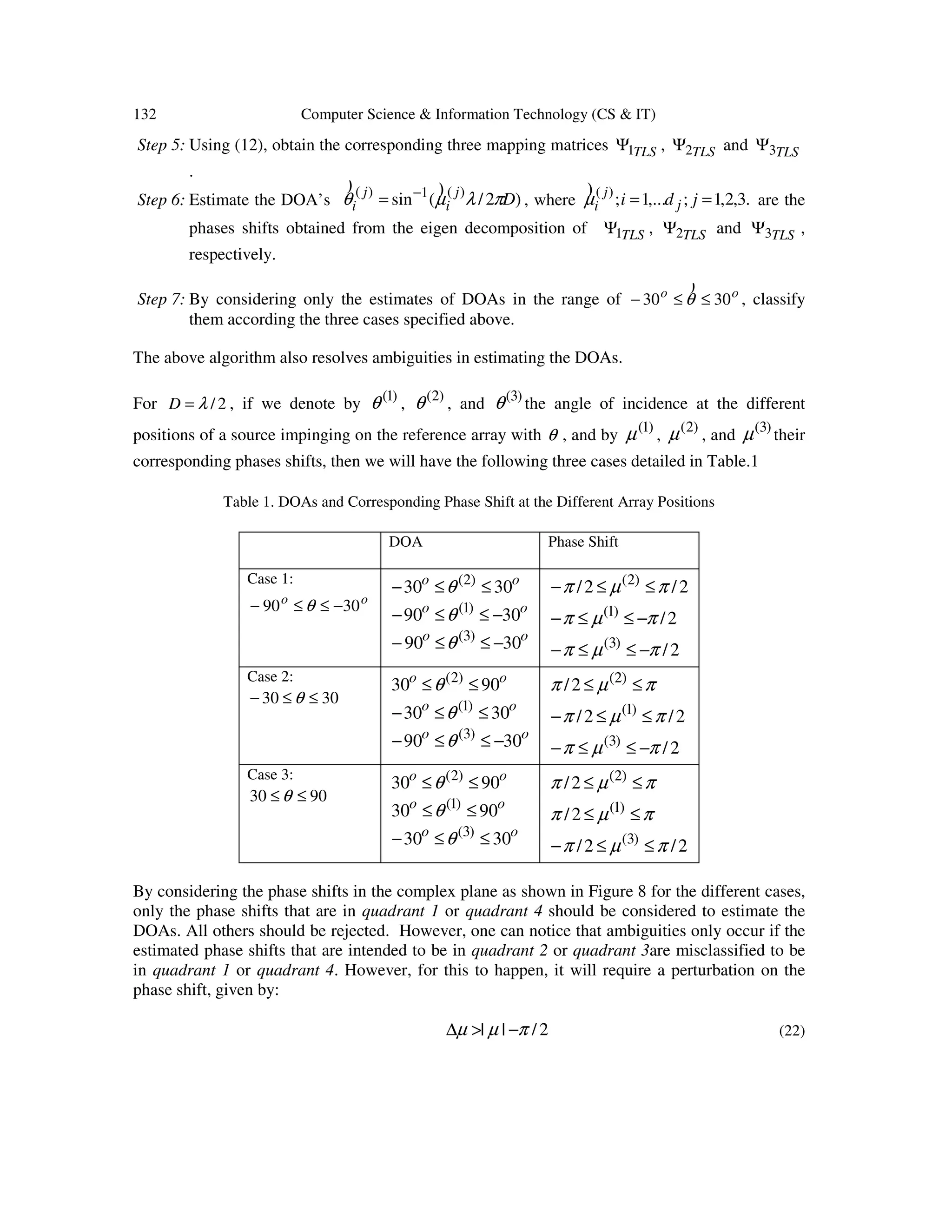
![128 Computer Science & Information Technology (CS & IT) For more than one source, the relationship between µσ and the SNR and number of snapshots n is more complicated [7]. Nevertheless due to the non-linear relationship between the phase shift and the DOA given by (1), the basic trend is that higher SNR and/or larger n are required to obtain more accurate DOA estimates or to distinguish between two or more close sources as the absolute of their angles of incidence increases. That is, ESPRIT is limited by its ability to resolve two closely spaced sources when their angles of incidence are along-side the ULA. In fact, for low SNR and limited number of snapshots, ESPRIT algorithm will fail in this case to determine that there are actually two sources present. It will indicate that there is only one source present. 2.3. Cyclic Ambiguities Consider the relation, given by (1), where we have tacitly assumed that )(λfD = holds perfectly. In practice however, due to measurement errors, this holds only approximately. Let D∆ , represent the error on D , this will introduce an error on the phase shift as λ θπ µ sin2 D∆ =∆ (18) Because the effective angular range of the ULA has a value oo 9090 ≤≤− θ , the phase shift has a value in the range πµπ <≤− . Since the inverse of the mapping ju e− →µ is aliased outside this range, then any error on the phase shift, given by (18), may introduce cyclic ambiguities in estimating the DOAs. For illustration purposes, suppose that )2/(56.0 λλ >=D and a source impinging on the array with o 85=θ , that correspond to a phase shift of 505.3=µ . This phase shift is cyclically equivalent to a phase shift of 777.2−=µ . ESPRIT will misinterpret this value and compute the estimated DOA, assuming 2/λ=D ,to be o 16.62−=θ which is very different from the true DOA at o 85 . In short, ambiguous errors due to misinterpretation of cyclically ambiguous phase shift occur in ESPRIT if || µπµ −>∆ . (19) Similarly, for low SNR and small number of snapshots, cyclic ambiguities may occur in estimating the DOAs for sources impinging on the array at an angle of incidence along-side the ULA. For 2/λ=D , consider the phase shift θπµ sin= , resulting for aθ close to o 90 , as shown in Figure 4 . It is noticeable that a small perturbation on the phase shift may lead to a phase shift πµ >1ˆ . This phase shift is cyclically equivalent to the phase shift µˆ . Again, ESPRIT algorithm will misinterpret the estimated phase and computes the estimated DOA at a value that is a very different from the true DOA.](https://image.slidesharecdn.com/csit76412-170207121240/75/RESOLVING-CYCLIC-AMBIGUITIES-AND-INCREASING-ACCURACY-AND-RESOLUTION-IN-DOA-ESTIMATION-USING-ARRAY-ROTATION-8-2048.jpg)
![Computer Science & Information Technology (CS & IT) 131 (b) (c) Figure 7. Computed DOAs as Function of the True DOAs at the Different Array Positions To be more specific the estimation of the DOAs is performed as follows: Step 1: Using (8), get estimates of the covariance matrices 1zzR ) , 2zzR ) , and 3zzR ) , obtained from the data collected at array positions1, 2and3, respectively. Step 2: Compute the generalized eigen decompositions of { }nZZ IR ,1 ) , { }nZZ IR ,2 ) , and { }nZZ IR ,3 ) , where nI is the identity matrix. Step 3: Using Akaike’s information criterion (AIC) or the minimum description length (MDL)[12], estimate the number of sources 1d , 2d and 3d at each array position. Note that ESPRIT may be limited by its ability to resolve two closely spaced sources when their angles of incidence are along-side the ULA, the estimation of the number of sources may vary at the different array positions. Step 4: Use(9)-(11) to obtain the signal spaces estimates, composed of the eigenvectors corresponding to the 1d , 2d , and 3d largest eigenvalues of 1ZZR ) , 2zzR ) , and 3zzR ) , respectively.](https://image.slidesharecdn.com/csit76412-170207121240/75/RESOLVING-CYCLIC-AMBIGUITIES-AND-INCREASING-ACCURACY-AND-RESOLUTION-IN-DOA-ESTIMATION-USING-ARRAY-ROTATION-11-2048.jpg)
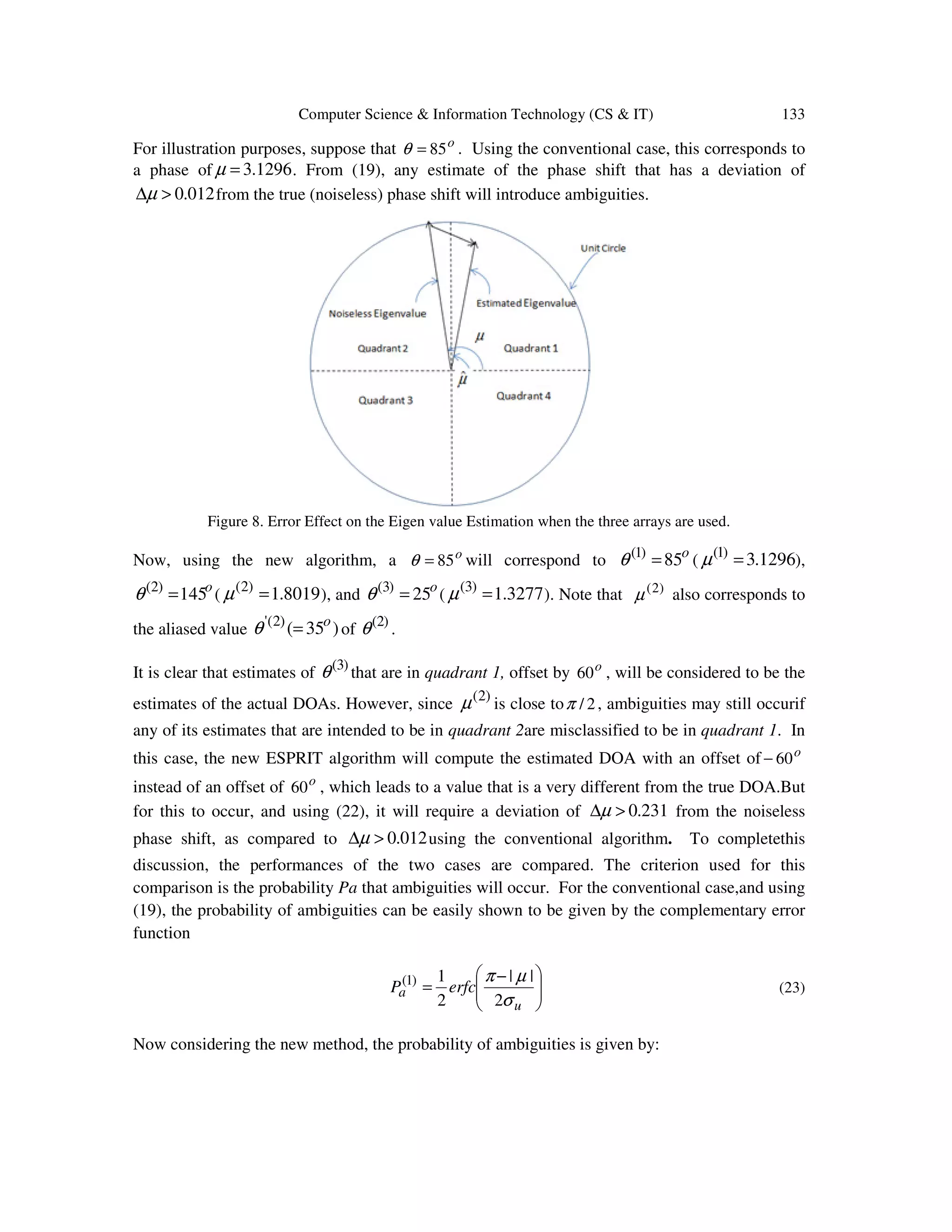
![Computer Science & Information Technology (CS & IT) 137 5. CONCLUSION The primary goal of this study has been to develop a procedure to resolve the cyclic ambiguities of the DOA estimates, and increase their resolution and accuracy. Although the new approach calls for the exploration of rotating the array and sampling the received data of signals at multiple positions, this disadvantage is overcome by the gain in accuracy and resolution in the DOA estimation, and the considerable improvement in reducing the ambiguities that are more likely to occur when the angle of incidence is along-side the ULA, especially for low SNR and small number of snapshots. Note that one can first only use the reference array (conventional method) in estimating the DOAs. If any estimates are found to be in the range oo 3090 −≤≤− θ ) or oo 9030 ≤≤ θ ) , then these estimates are considered to be coarse estimates, and the array will be rotated by o 60 and o 60− to obtain estimates at a finer scale. REFERENCES [1] E. Tuncer and B. Friedlander, (2009) Classical and Modern Direction-of-Arrival Estimation, Ed. Elsevier, USA. [2] F. F. Gao and A. B. Gershman, (2005) “A generalized ESPRIT approach to direction-of-arrival estimation,” IEEE Signal Processing Letters, vol. 12, no. 3, pp. 254-257. [3] N. P. Waweru, D. B. O. Konditi, P. K. Langat, (2014) “Performance Analysis of MUSIC, Root- MUSIC and ESPRIT DOA Estimation Algorithm,” International Journal of Electrical, Computer, Energetic, Electronic and Communication Engineering, Vol. 8, No:1, pp. 209-216. [4] M. H. Bhede, D. G. Ganage, S. A. Wagh, (2015) “Performance Analysis of MUSIC and Smooth MUSIC Algorithm for DOA Estimation,” International Journal on Recent and Innovation Trends in Computing and Communication, Vol. 3, Issue. 7, pp. 4397-4402. [5] C. L. Srinidh, S. A. Hariprasad, (2012) “Comparative Study on Performance Analysis ofHigh Resolution Direction of Arrival Estimation Algorithms,” International Journal of Advanced Research in Computer Engineering & Technology, Volume 1, Issue 4, June 2012, pp. 67-79. [6] K.T. Wong, M. D. Zoltowski,(1998) “Direction finding with sparse rectangular dual-size spatial invariance array”, IEEE Trans. Aerosp. Electron. Syst., 34, (4), pp. 1320– 1327. [7] A. N. Lemma, A. J. van der Veen, and E. F. Deprettere, (1999) “ Multiresolution ESPRIT Algorithm,” IEEE Transactions on Signal Processing, Vol. 47, No. 6, June 1999, pp. 1722-1726. [8] V. I. Vasylyshyn,(2005) “Unitary ESPRIT-based DOA estimation using sparse linear dual size spatial invariance array”. Proc. European Radar Conf., Paris, France, pp. 157– 160. [9] Tan, C. M., et al, (2002) “Ambiguity in MUSIC and ESPRIT for direction of arrival estimation,” Electronics Letters, vol.38, no. 24, pp. 1598- 1600. [10] K. Yang, Z. Zhao, X. Zhu, and Q. H. Liu, (2013) “Resolving ambiguities in DOA estimation by optimizing the element orientations,” in Proc. IEEE Antennas Propag. Soc. Int. Symp. (APSURSI), Jul. 2013, pp. 1326–1327.](https://image.slidesharecdn.com/csit76412-170207121240/75/RESOLVING-CYCLIC-AMBIGUITIES-AND-INCREASING-ACCURACY-AND-RESOLUTION-IN-DOA-ESTIMATION-USING-ARRAY-ROTATION-17-2048.jpg)
![138 Computer Science & Information Technology (CS & IT) [11] R. Roy and T. Kailath, (1989) “ESPRIT-Estimation of Signal Parameters Via Rotational Invariance Techniques,” IEEE Transactions on Acoustics, Speech and Signal Processing, Vol. 37. No. 7, July 1989, pp. 984-995. [12] D. B. Williams, (1999) “Detection: Determining the number of sources,” in Digital Signal Processing Handbook, V. K. Madisetti and D. B. Williams, Eds. Boca Raton, FL: CRC. AUTHORS Abdelhamid Djouadi received the B.S. degree in electrical engineering from the University of Sciences and Technologies, Oran, Algeria, in 1980, and the M.S. and Ph.D. degree in electrical engineering from The Ohio State University, Columbus, OH, USA, in 1983 and 1987, respectively. After a successful academic career, since 1997, he has been with Nokia (former Alcatel-Lucent Technologies) as a technical lead driving improvement in 4G and 3G products. His research interests include wireless telecommunication, pattern recognition, sensor array, and signal processing. Nebojsa I. Jaksic received the Dipl. Ing. degree in electrical engineering from Belgrade University in 1984, the M.S. in electrical engineering in 1988, the M.S. in industrial engineering in 1992, and the Ph.D. in industrial engineering in 2000 from The Ohio State University, Columbus, OH, USA. He is currently Professor at Colorado State University-Pueblo. Dr. Jaksic has published over 60 papers and holds two patents. He is a registered Professional Engineer with the State of Colorado. Dr. Jaksic is a senior member of IEEE and SME, and a member of ASEE. His research interests include robotics, automation, and nanotechnology.](https://image.slidesharecdn.com/csit76412-170207121240/75/RESOLVING-CYCLIC-AMBIGUITIES-AND-INCREASING-ACCURACY-AND-RESOLUTION-IN-DOA-ESTIMATION-USING-ARRAY-ROTATION-18-2048.jpg)