Downloaded 231 times
![Quicksort • Quicksort pros [advantage]: – Sorts in place – Sorts O(n lg n) in the average case – Very efficient in practice , it’s quick • Quicksort cons [disadvantage]: – Sorts O(n2 ) in the worst case – And the worst case doesn’t happen often … sorted](https://image.slidesharecdn.com/quicksortdiscussionandanalysis-150830134127-lva1-app6891/75/Quick-sort-Algorithm-Discussion-And-Analysis-6-2048.jpg)
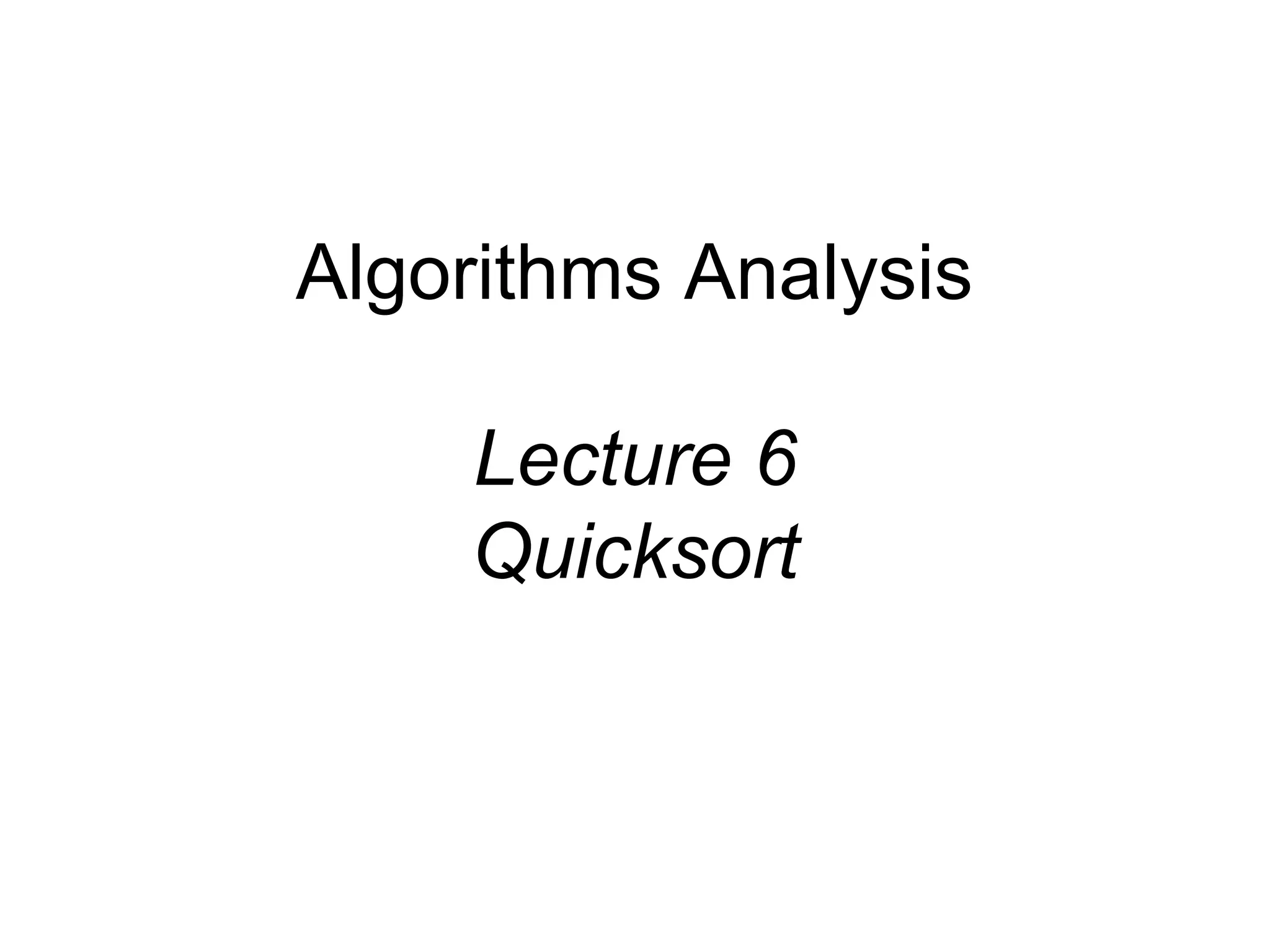
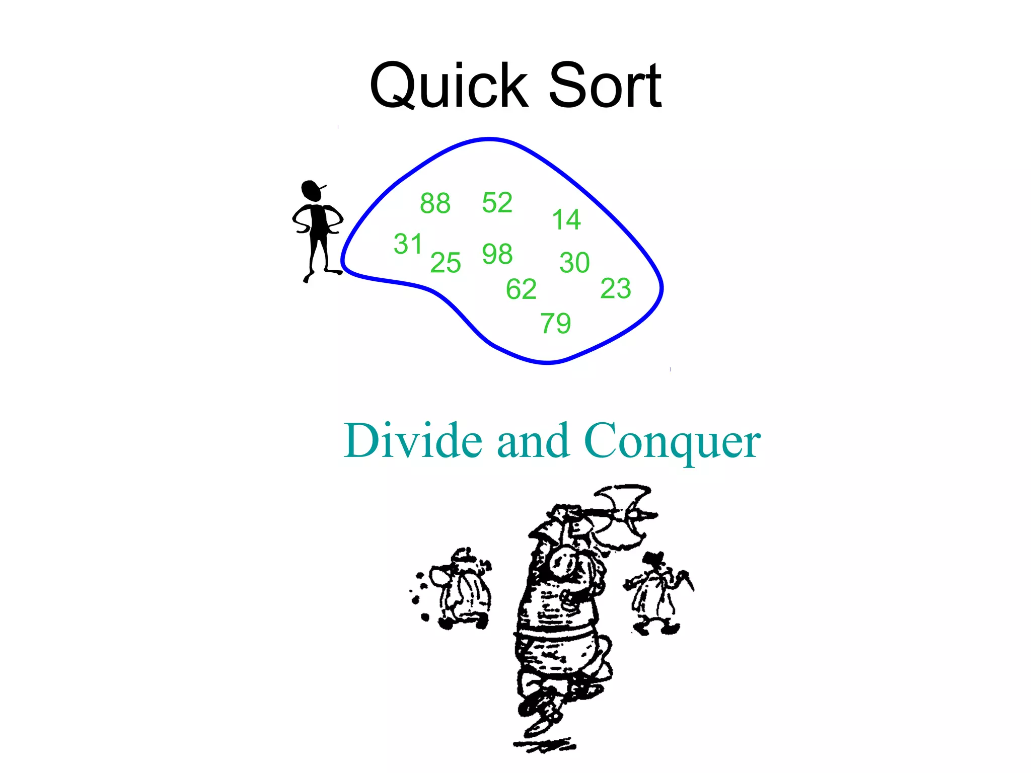
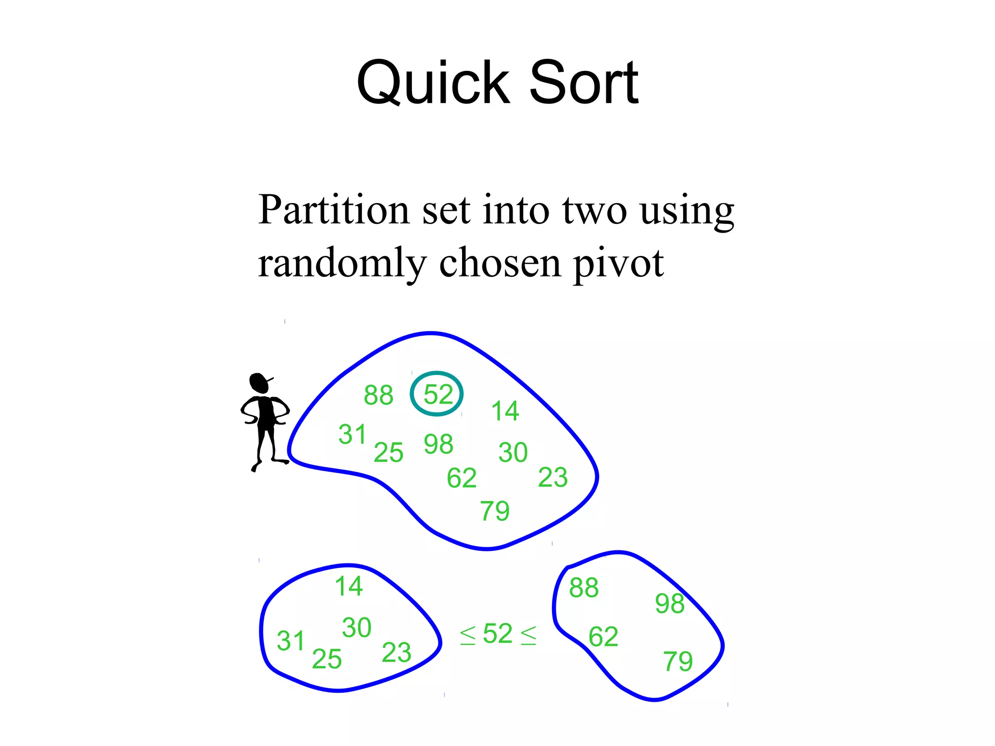
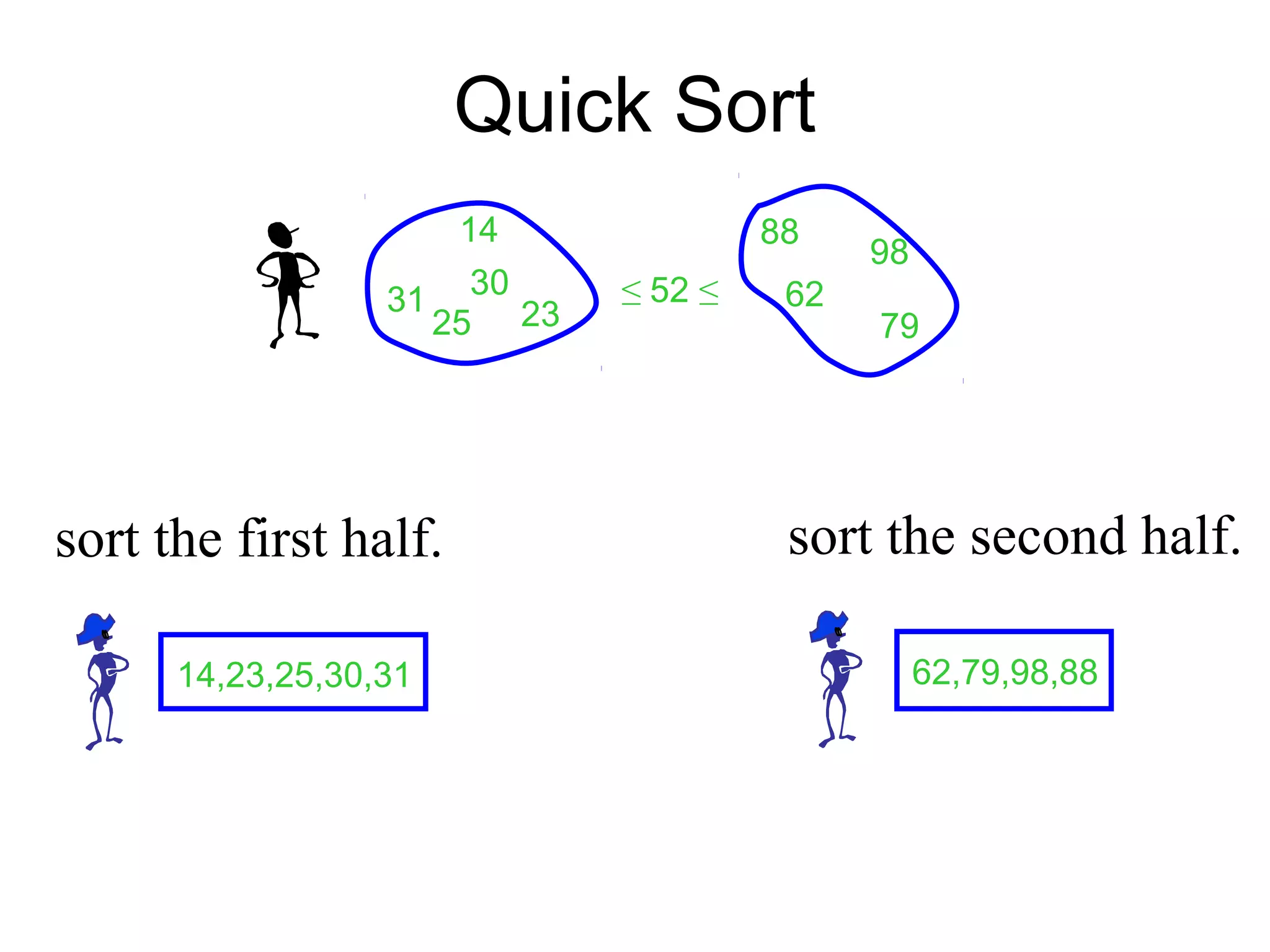
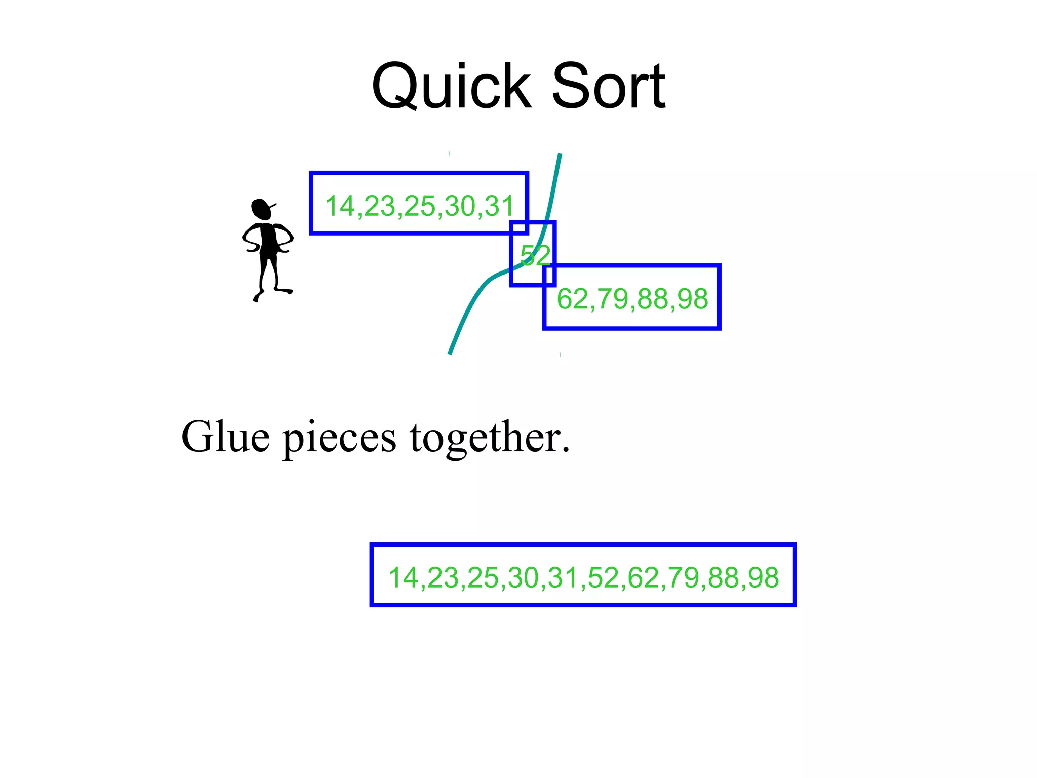
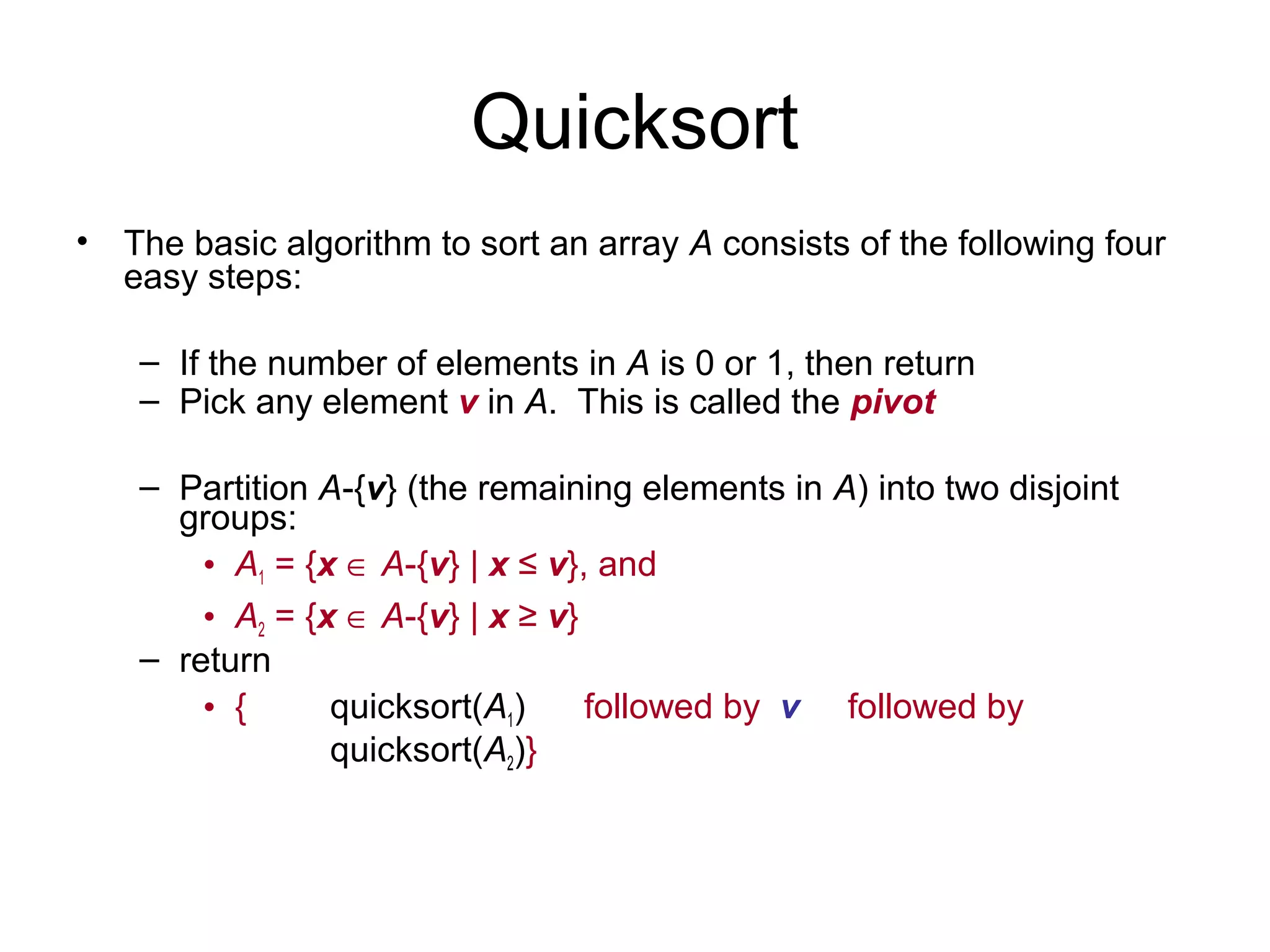
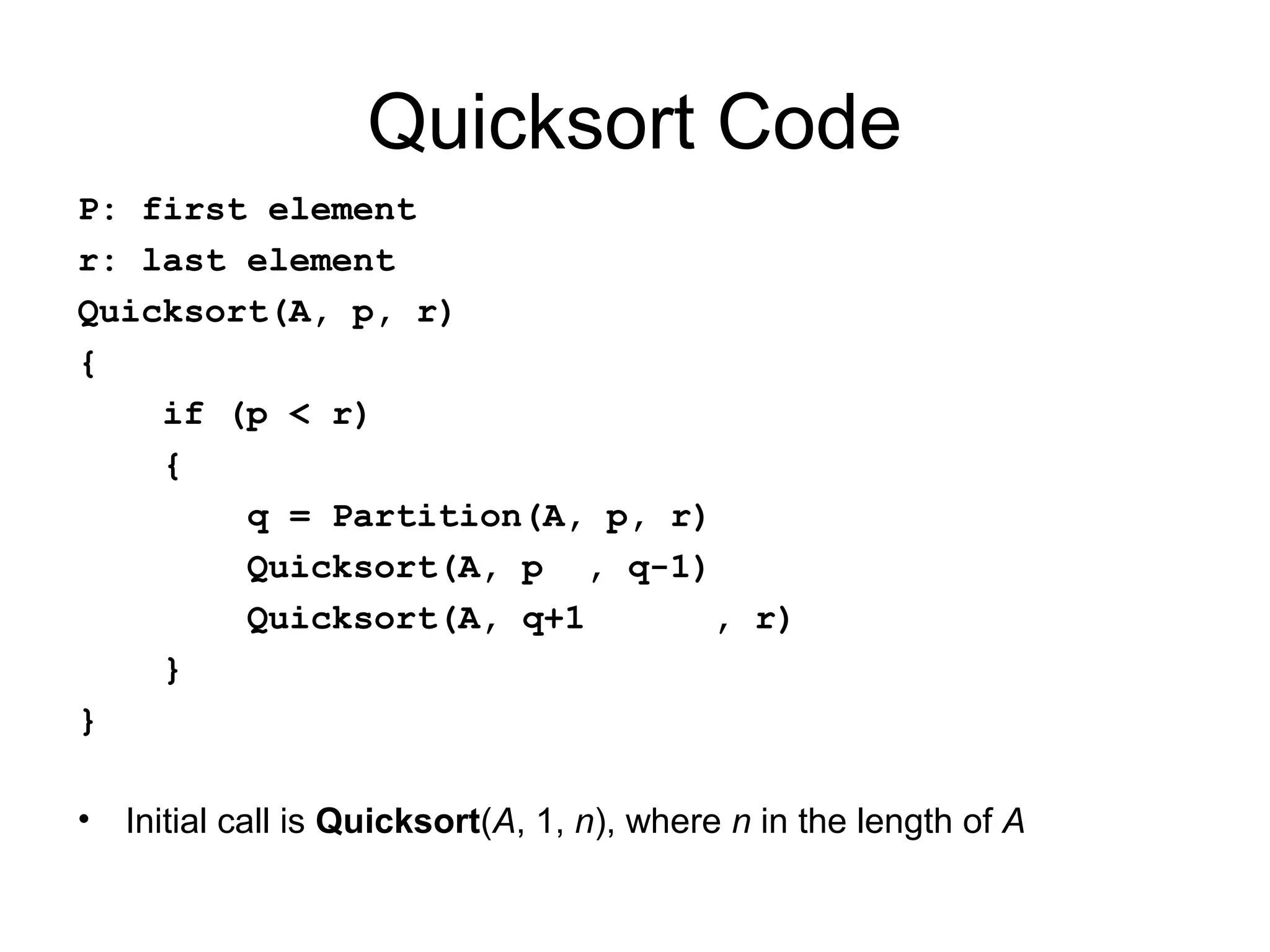
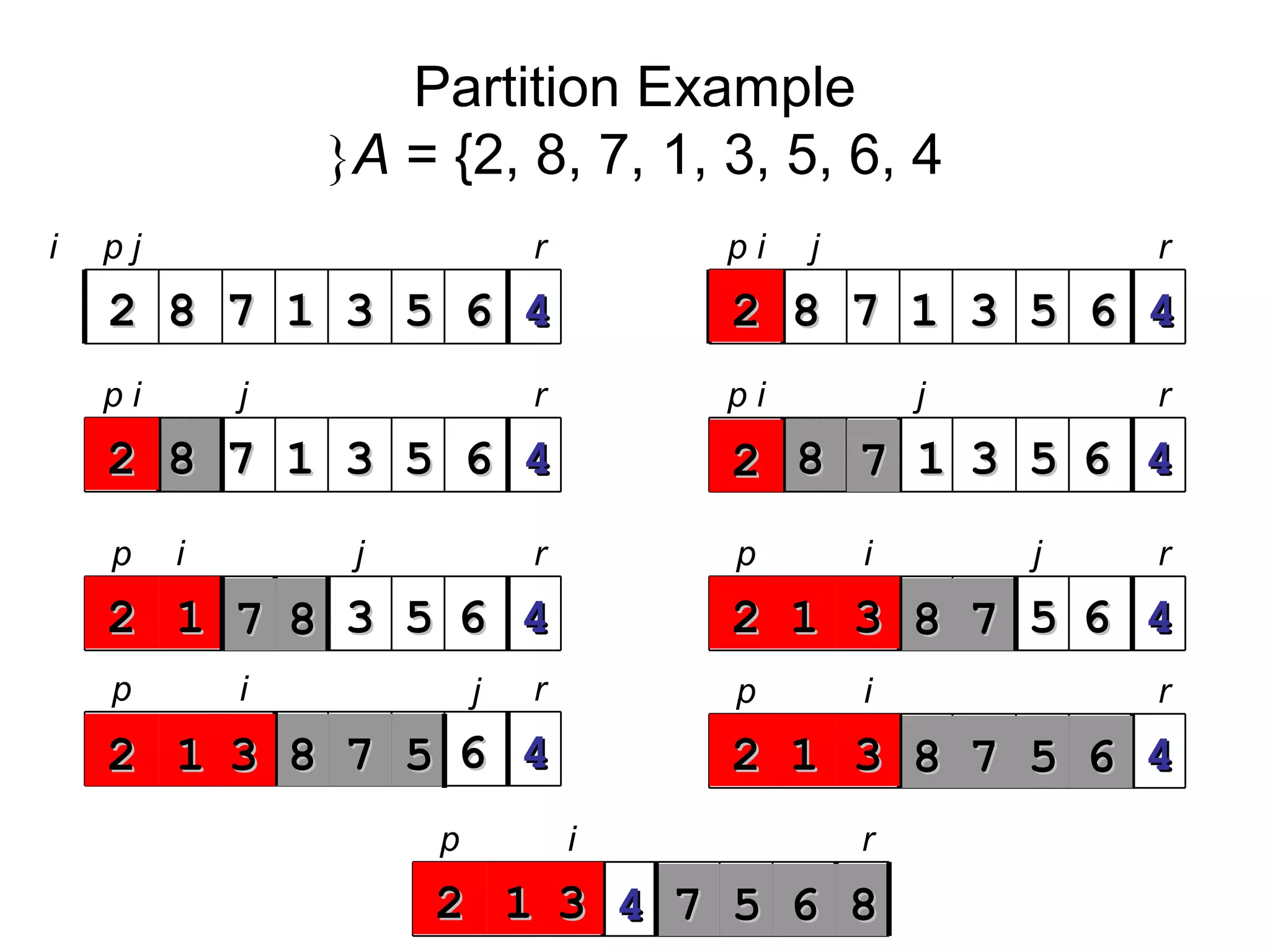
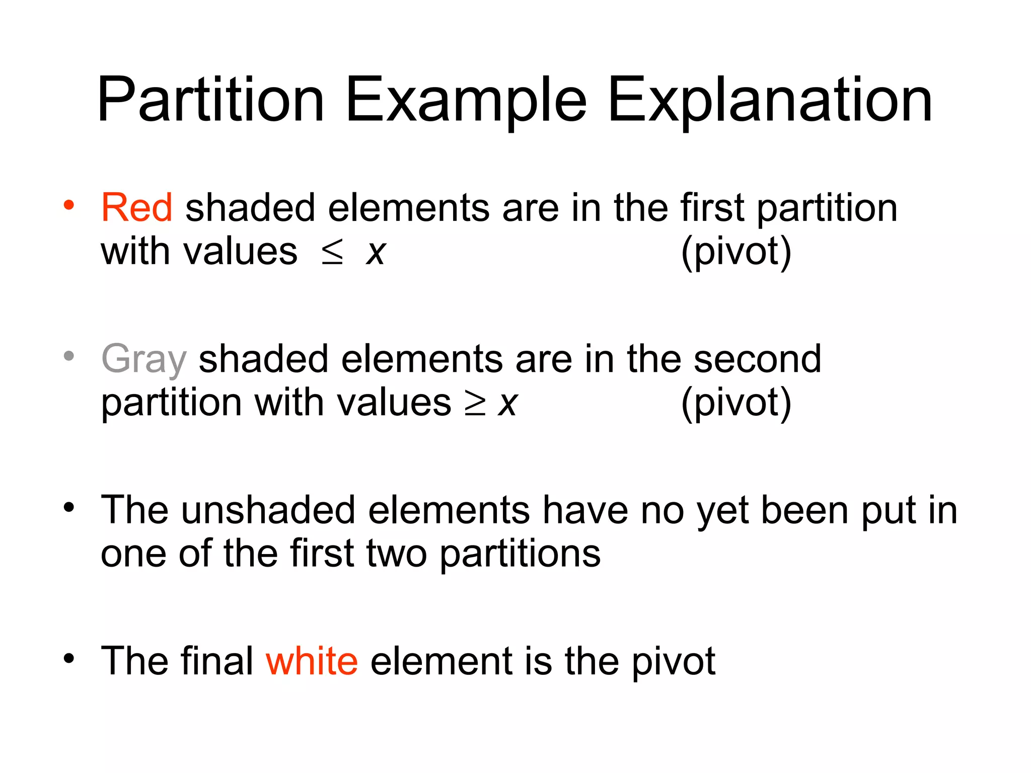
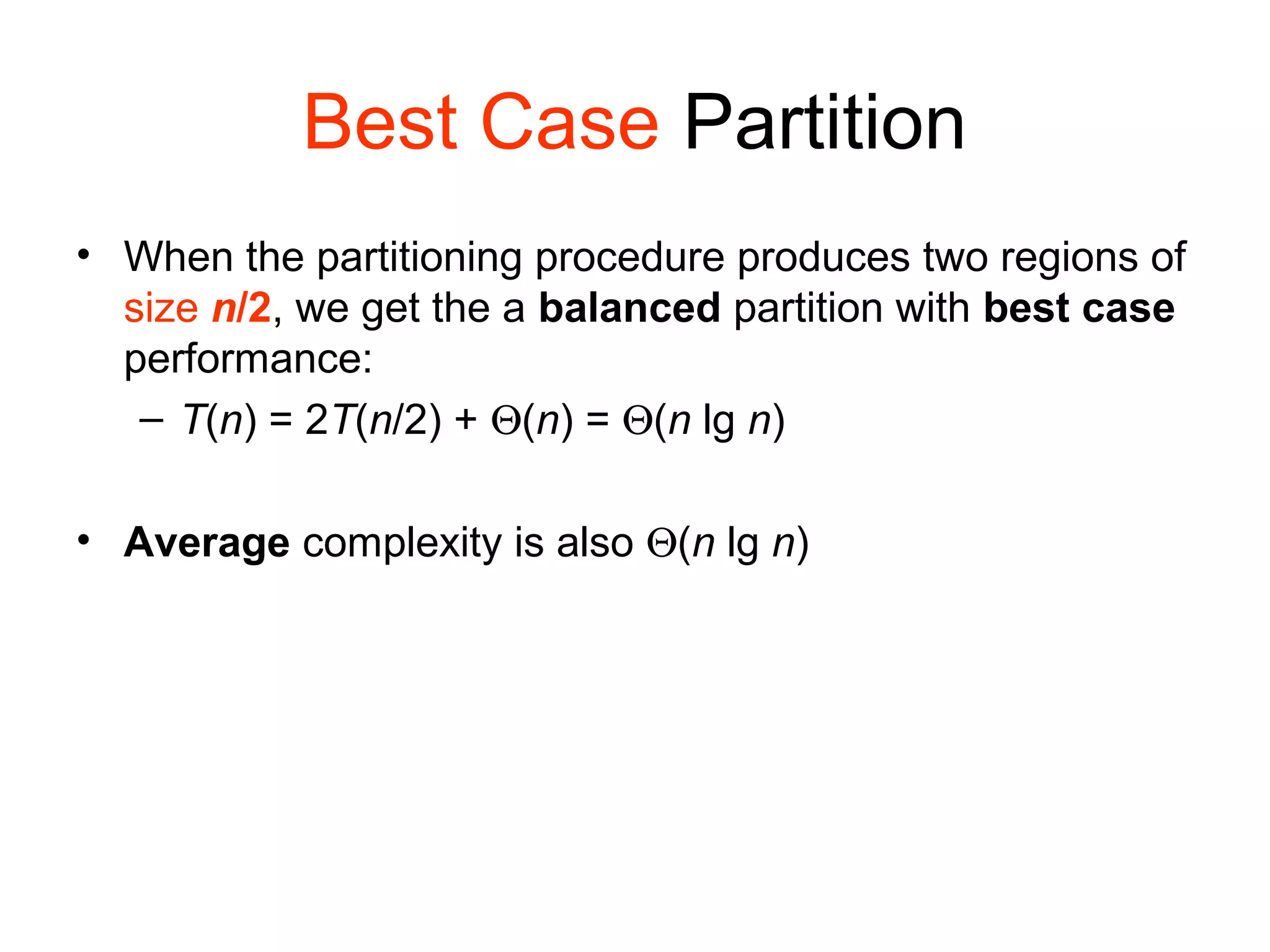
![Quicksort • Another divide-and-conquer algorithm: • Divide: A[p…r] is partitioned (rearranged) into two nonempty subarrays A[p…q-1] and A[q+1…r] s.t. each element of A[p…q-1] is less than or equal to each element of A[q+1…r]. Index q is computed here, called pivot. • Conquer: two subarrays are sorted by recursive calls to quicksort. • Combine: unlike merge sort, no work needed since the subarrays are sorted in place already.](https://image.slidesharecdn.com/quicksortdiscussionandanalysis-150830134127-lva1-app6891/75/Quick-sort-Algorithm-Discussion-And-Analysis-7-2048.jpg)

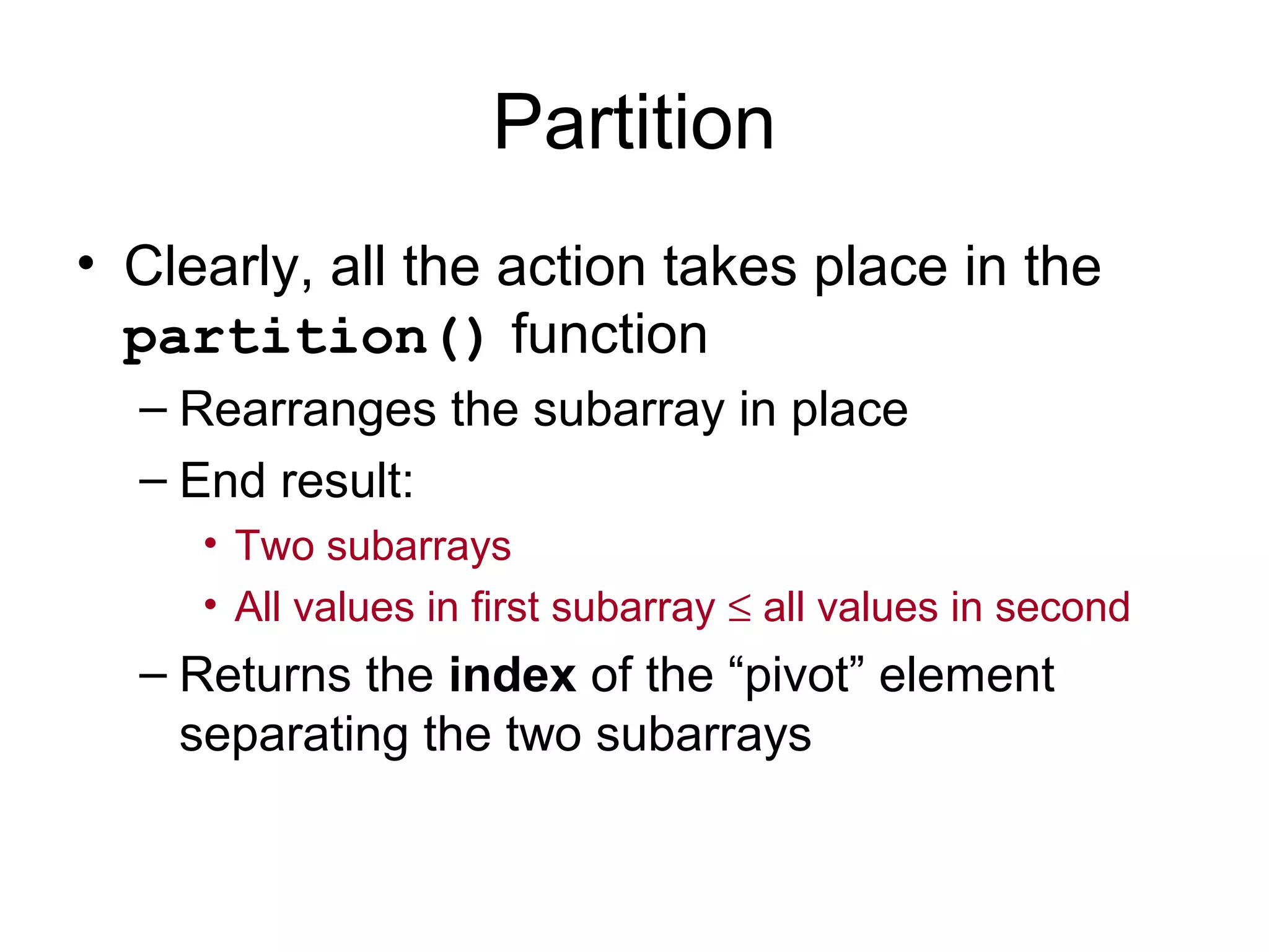
![Partition Code Partition(A, p, r) { x = A[r] // x is pivot i = p - 1 for j = p to r – 1 { do if A[j] <= x then { i = i + 1 exchange A[i] ↔ A[j] } } exchange A[i+1] ↔ A[r] return i+1 } partition() runs in O(n) time](https://image.slidesharecdn.com/quicksortdiscussionandanalysis-150830134127-lva1-app6891/75/Quick-sort-Algorithm-Discussion-And-Analysis-12-2048.jpg)
![Choice Of Pivot Three ways to choose the pivot: • Pivot is rightmost element in list that is to be sorted – When sorting A[6:20], use A[20] as the pivot – Textbook implementation does this • Randomly select one of the elements to be sorted as the pivot – When sorting A[6:20], generate a random number r in the range [6, 20] – Use A[r] as the pivot](https://image.slidesharecdn.com/quicksortdiscussionandanalysis-150830134127-lva1-app6891/75/Quick-sort-Algorithm-Discussion-And-Analysis-15-2048.jpg)
![Choice Of Pivot • Median-of-Three rule - from the leftmost, middle, and rightmost elements of the list to be sorted, select the one with median key as the pivot – When sorting A[6:20], examine A[6], A[13] ((6+20)/2), and A[20] – Select the element with median (i.e., middle) key – If A[6].key = 30, A[13].key = 2, and A[20].key = 10, A[20] becomes the pivot – If A[6].key = 3, A[13].key = 2, and A[20].key = 10, A[6] becomes the pivot](https://image.slidesharecdn.com/quicksortdiscussionandanalysis-150830134127-lva1-app6891/75/Quick-sort-Algorithm-Discussion-And-Analysis-16-2048.jpg)
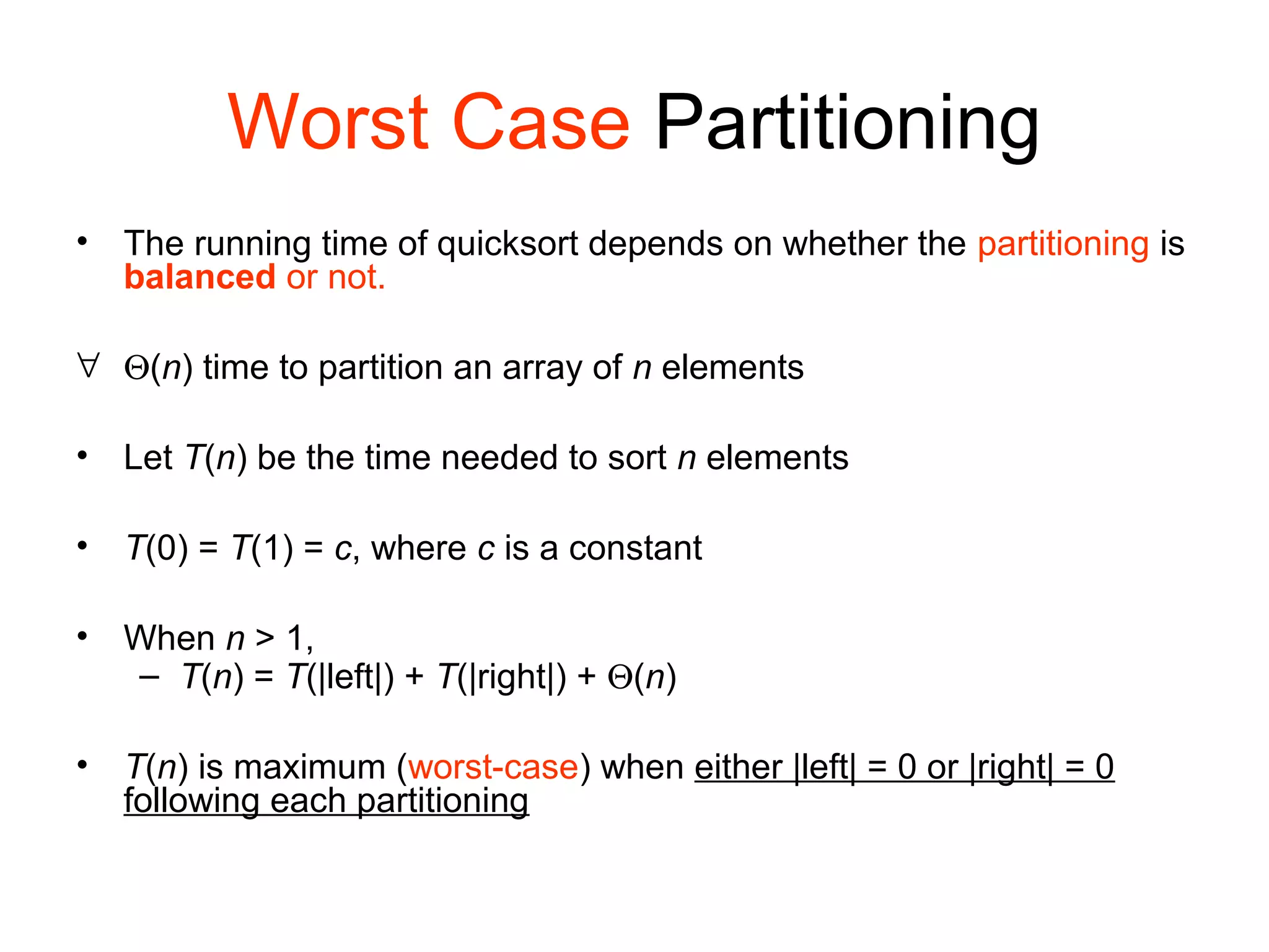
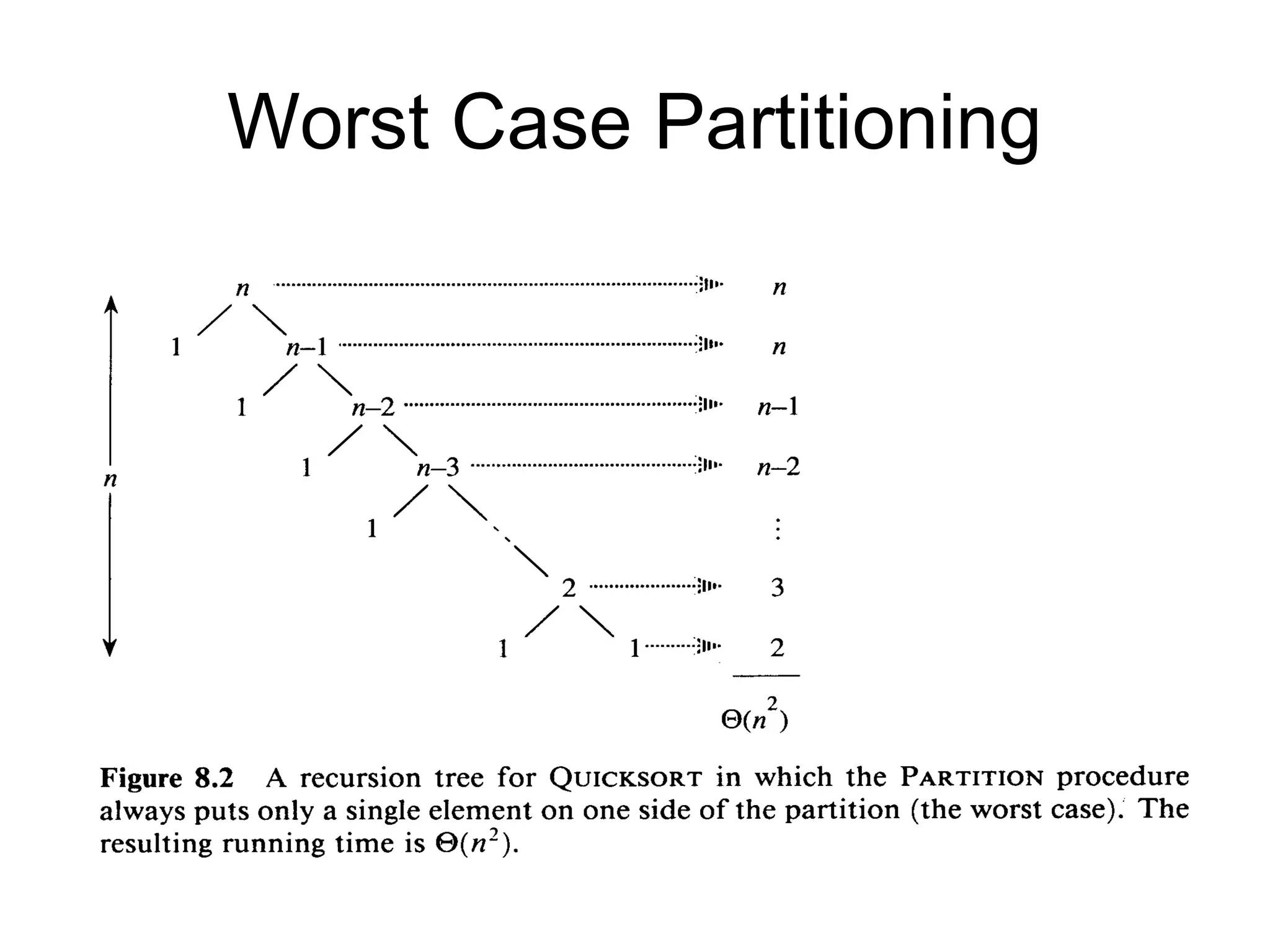
![Worst Case Partitioning • Worst-Case Performance (unbalanced): – T(n) = T(1) + T(n-1) + Θ(n) • partitioning takes Θ(n) = [2 + 3 + 4 + …+ n-1 + n ]+ n = = [∑k = 2 to n k ]+ n = Θ(n2 ) • This occurs when – the input is completely sorted • or when – the pivot is always the smallest (largest) element )(2/)1(...21 2 1 nnnnk n k Θ=+=+++=∑=](https://image.slidesharecdn.com/quicksortdiscussionandanalysis-150830134127-lva1-app6891/75/Quick-sort-Algorithm-Discussion-And-Analysis-19-2048.jpg)
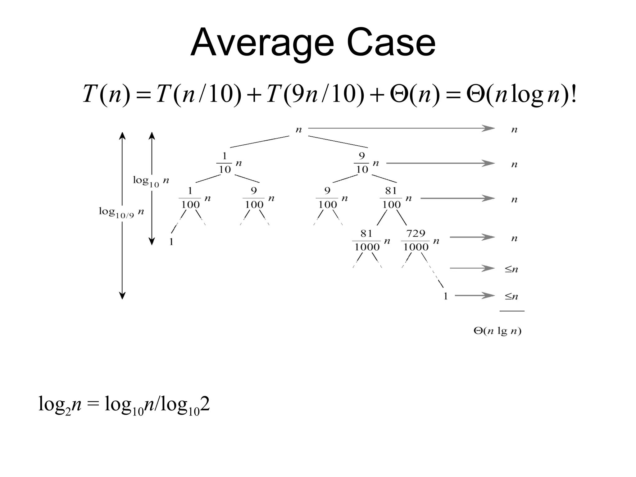
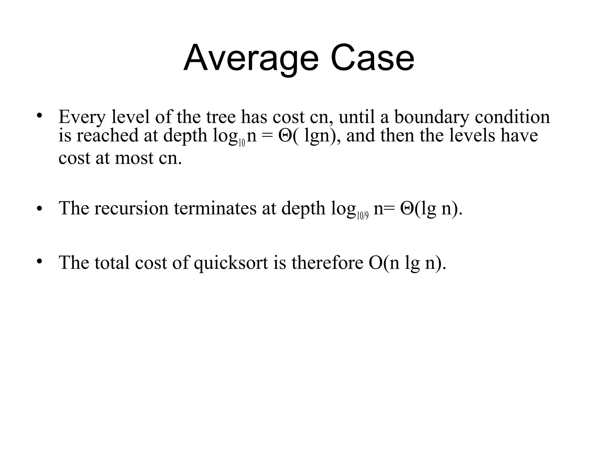
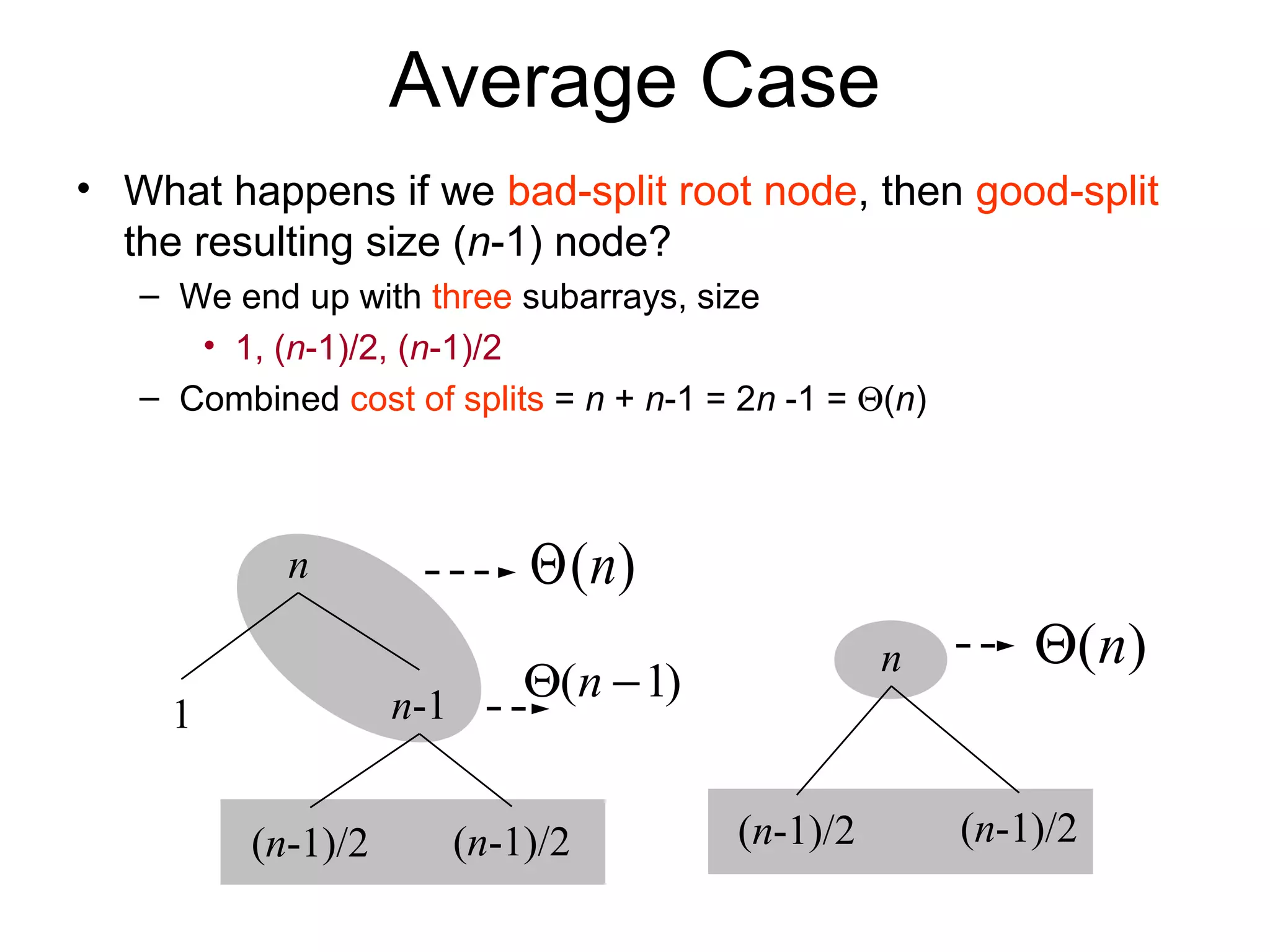
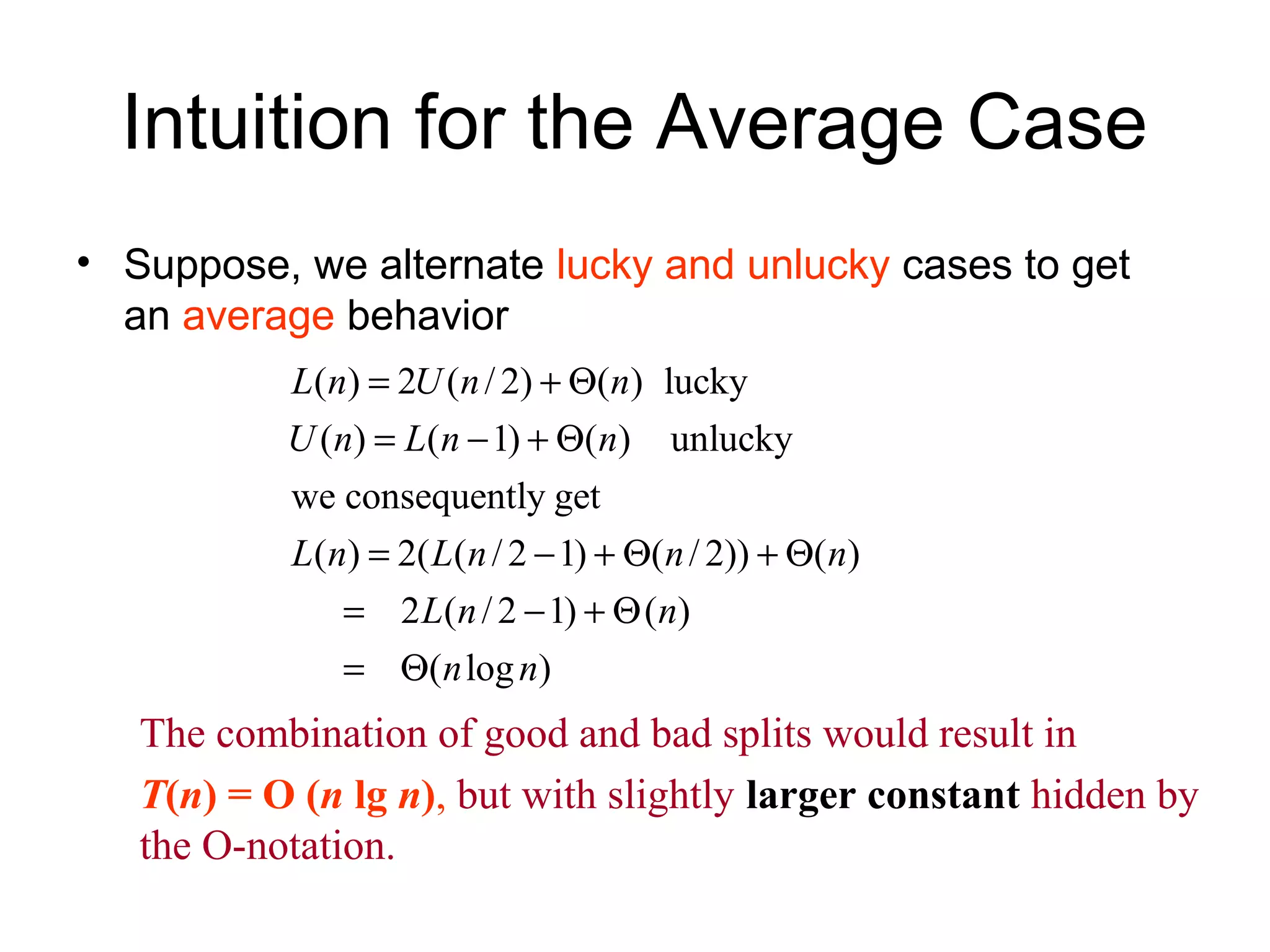
![Average Case • Assuming random input, average-case running time is much closer to Θ(n lg n) than Θ(n2 ) • First, a more intuitive explanation/example: – Suppose that partition() always produces a 9-to-1 proportional split. This looks quite unbalanced! – The recurrence is thus: T(n) = T(9n/10) + T(n/10) + Θ(n) = Θ(nlg n)? [Using recursion tree method to solve]](https://image.slidesharecdn.com/quicksortdiscussionandanalysis-150830134127-lva1-app6891/75/Quick-sort-Algorithm-Discussion-And-Analysis-22-2048.jpg)
![Randomized Quicksort • An algorithm is randomized if its behavior is determined not only by the input but also by values produced by a random-number generator. • Exchange A[r] with an element chosen at random from A[p…r] in Partition. • This ensures that the pivot element is equally likely to be any of input elements. • We can sometimes add randomization to an algorithm in order to obtain good average-case performance over all inputs.](https://image.slidesharecdn.com/quicksortdiscussionandanalysis-150830134127-lva1-app6891/75/Quick-sort-Algorithm-Discussion-And-Analysis-27-2048.jpg)
![Randomized Quicksort Randomized-Partition(A, p, r) 1. i ← Random(p, r) 2. exchange A[r] ↔ A[i] 3. return Partition(A, p, r) Randomized-Quicksort(A, p, r) 1. if p < r 2. then q ← Randomized-Partition(A, p, r) 3. Randomized-Quicksort(A, p , q-1) 4. Randomized-Quicksort(A, q+1, r) pivot swap](https://image.slidesharecdn.com/quicksortdiscussionandanalysis-150830134127-lva1-app6891/75/Quick-sort-Algorithm-Discussion-And-Analysis-28-2048.jpg)
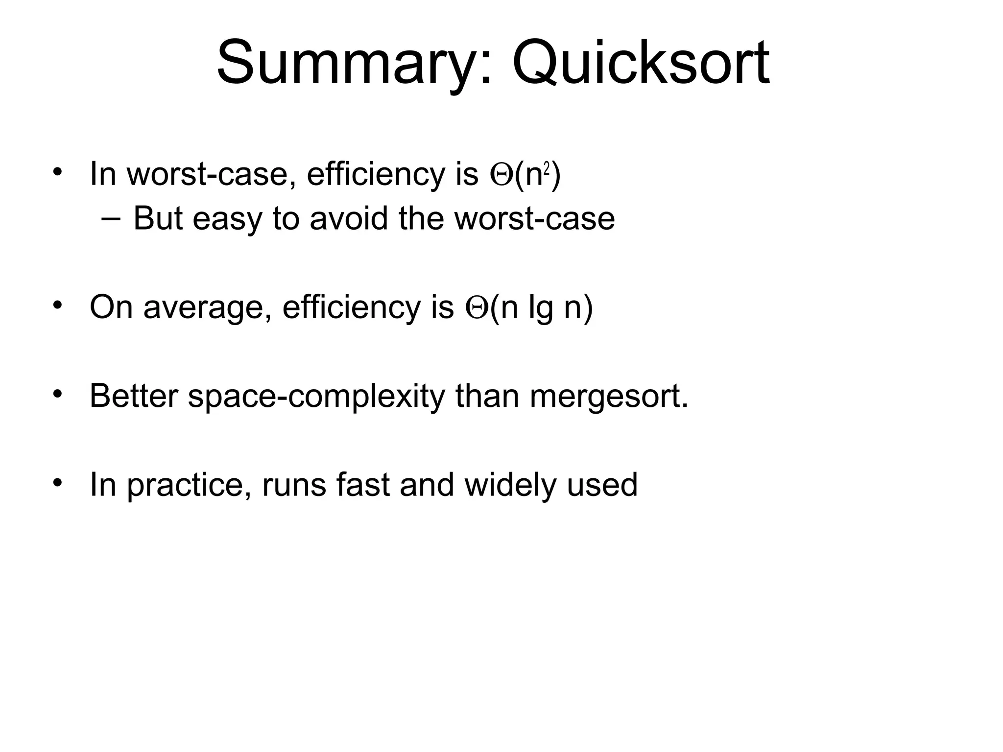

Quicksort is a divide-and-conquer algorithm that works by partitioning an array around a pivot element and recursively sorting the subarrays. In the average case, it has an efficiency of Θ(n log n) time as the partitioning typically divides the array into balanced subproblems. However, in the worst case of an already sorted array, it can be Θ(n^2) time due to highly unbalanced partitioning. Randomizing the choice of pivot helps avoid worst-case scenarios and achieve average-case efficiency in practice, making quicksort very efficient and commonly used.