program partitioning and scheduling IN Advanced Computer Architecture

Advanced Computer Architecture Program Partitioning and Scheduling

Program partitioning The transformation of sequentially coded program into a parallel executable form can b done manually by the programmer using explicit parallelism or by a compiler detecting implicit parallelism automatically. Program partitioning determines whether the given program can be partitioned or split into pieces that can be executed in parallel or follow a certain prespecified order of execution.

Program Partitioning & Scheduling The size of the parts or pieces of a program that can be considered for parallel execution can vary. The sizes are roughly classified using the term “granule size,” or simply “granularity.” The simplest measure, for example, is the number of instructions in a program part. Grain sizes are usually described as fine, medium or coarse, depending on the level of parallelism involved.

Latency Latency is the time required for communication between different subsystems in a computer. Memory latency, for example, is the time required by a processor to access memory. Synchronization latency is the time required for two processes to synchronize their execution. Communication latency is the interprocessor communication.

Levels of Parallelism Jobs or programs Instructions or statements Non-recursive loops or unfolded iterations Procedures, subroutines, tasks, or coroutines Subprograms, job steps or related parts of a program } } Coarse grain Medium grain }Fine grain Increasing communication demand and scheduling overhead Higher degree of parallelism

Instruction Level Parallelism This fine-grained, or smallest granularity level typically involves less than 20 instructions per grain. The number of candidates for parallel execution varies from 2 to thousands, with about five instructions or statements (on the average) being the average level of parallelism. Advantages: The exploitation of fine-grain parallelism can be assisted by an optimizing compiler which should be able to automatically detect parallelism and translate the source code to a parallel form which can be recognized by the run- time system.

Loop-level Parallelism Typical loop has less than 500 instructions. If a loop operation is independent between iterations, it can be handled by a pipeline, or by a SIMD machine. Loop Level Parallelism is the most optimized program construct to execute on a parallel or vector machine Some loops (e.g. recursive) are difficult to handle. Loop-level parallelism is still considered fine grain computation.

Procedure-level Parallelism Medium-sized grain; usually less than 2000 instructions. Detection of parallelism is more difficult than with smaller grains; Interprocedural dependence analysis is difficult and history-sensitive. Communication requirement less than instruction- level SPMD (single procedure multiple data)execution mode is a special case at this level. Multitasking belongs to this level.

Subprogram-level Parallelism Job step level; grain typically has thousands of instructions; medium- or coarse-grain level. Job steps can overlap across different jobs. Multiprogramming conducted at this level. In the past ,parallelism at this level has been exploited by algorithm or programmers, rather then by compiler. We do not have good compiler available to exploit medium- or coarse-grain parallelism at present.

Job or Program-Level Parallelism Corresponds to execution of essentially independent jobs or programs on a parallel computer. The grain size can be large as tens of thousand of instruction in a single program. For supercomputers with a small number of very powerful processors, such coarse-grain parallelism is practical. Time sharing or space-sharing multiprocessor explore this level of parallelism. Job level parallelism is handled by program loader or by the operating system.

Summary Fine-grain exploited at instruction or loop levels, assisted by the compiler. Medium-grain (task or job step) requires programmer and compiler support. Coarse-grain relies heavily on effective OS support. Shared-variable communication used at fine- and medium- grain levels. Message passing can be used for medium- and coarse- grain communication, but fine-grain really need better technique because of heavier communication requirements.

Communication Latency Balancing granularity and latency can yield better performance. Various latencies attributed to machine architecture, technology, and communication patterns used. Latency imposes a limiting factor on machine scalability. Ex. Memory latency increases as memory capacity increases, limiting the amount of memory that can be used with a given tolerance for communication latency.

Interprocessor Communication Latency Needs to be minimized by system designer Affected by signal delays and communication patterns Ex. n communicating tasks may require n (n - 1)/2 communication links, and the complexity grows quadratically, effectively limiting the number of processors in the system.

Communication Patterns Determined by algorithms used and architectural support provided Patterns include permutations broadcast multicast conference Tradeoffs often exist between granularity of parallelism and communication demand.

Grain Packing and Scheduling Two questions: How can I partition a program into parallel “pieces” to yield the shortest execution time? What is the optimal size of parallel grains? There is an obvious tradeoff between the time spent scheduling and synchronizing parallel grains and the speedup obtained by parallel execution. One approach to the problem is called “grain packing.”

EENG-630 - Chapter 2 Grain packing and scheduling The grain size problem requires determination of both the number of partitions and the size of grains in a parallel problem Solution is problem dependent and machine dependent Want a short schedule for fast execution of subdivided program modules

EENG-630 - Chapter 2 Grain determination and scheduling optimization Step 1: Construct a fine-grain program graph Step 2: Schedule the fine-grain computation Step 3: Grain packing to produce coarse grains Step 4: Generate a parallel schedule based on the packed graph

Program Graphs and Packing A program graph is similar to a dependence graph Nodes = { (n,s) }, where n = node name, s = size (larger s = larger grain size). Edges = { (v,d) }, where v = variable being “communicated,” and d = communication delay. Packing two (or more) nodes produces a node with a larger grain size and possibly more edges to other nodes. Packing is done to eliminate unnecessary communication delays or reduce overall scheduling overhead.

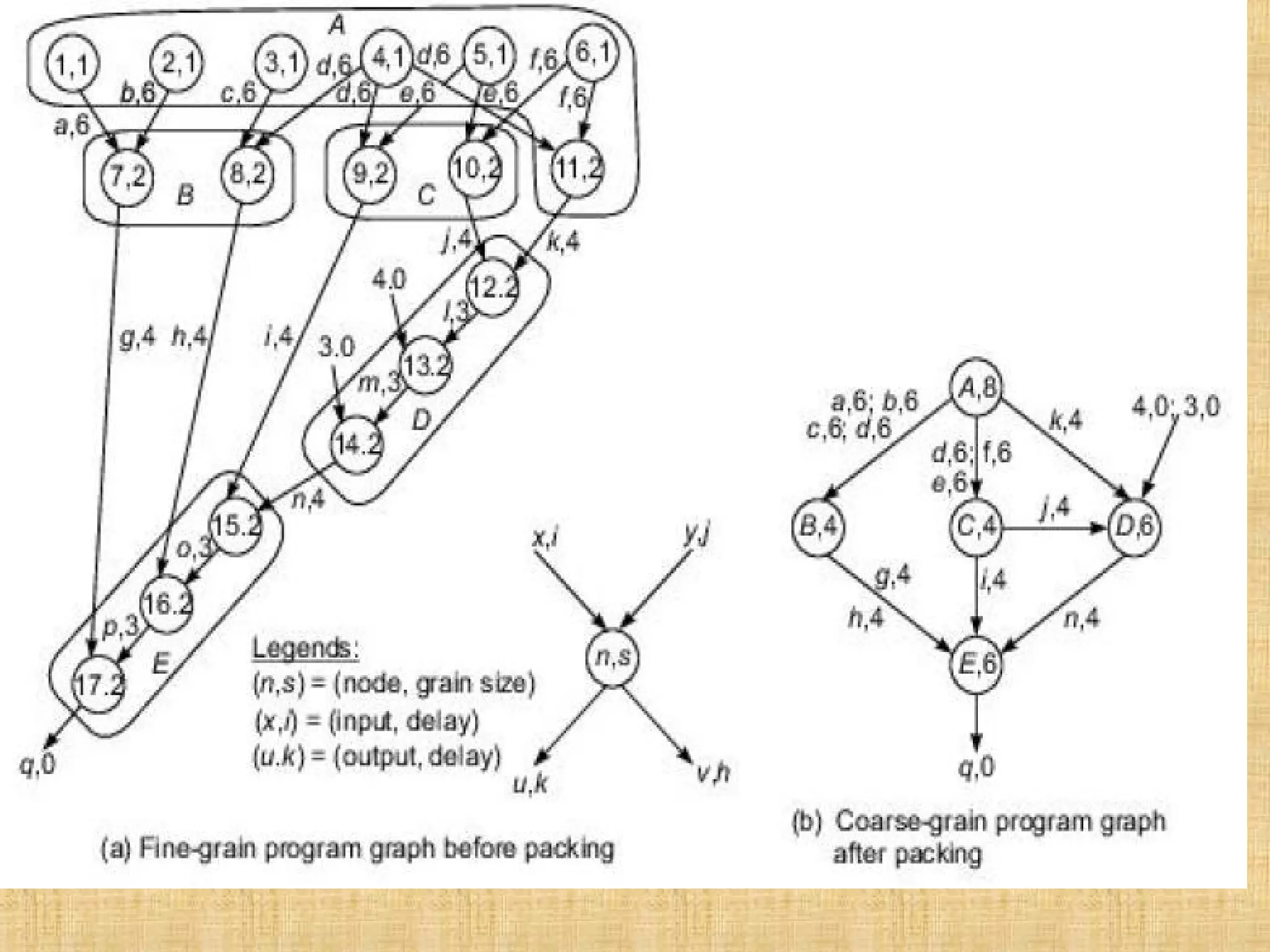
The basic concept of program partitioning is introduced here . In Fig. we show an example program graph in two different grain sizes. A program graph shows the structure of a program. It is very similar to the dependence graph . Each node in the program graph corresponds to a computational unit in the program. The grain size is measured by the number of basic machine cycle[including both processor and memory cycles] needed to execute all the operations within the node. We denote each node in Fig. by a pair (n,s) , where n is the node name {id} and s is the grain size of the node. Thus grain size reflects the number of computations involved in a program segment. Fine-grain nodes have a smaller grain size. and coarse-grain nodes have a larger grain size.

The edge label (v,d) between two end nodes specifies the output variable v from the source node or the input variable to the destination node , and the communication delay d between them.  This delay includes all the path delays and memory latency involved. There are 17 nodes in the fine-grain program graph (Fig. a) and 5 in the coarse-grain program graph (Fig. b]. The coarse-grain node is obtained by combining {grouping} multiple fine-grain nodes.  The fine grain corresponds to the following program:

Nodes l, 2, 3, 4, 5, and 6 are memory reference (data fetch} operations. Each takes one cycle to address and six cycles to fetch from memory. All remaining nodes (7 to 17) are CPU operations, each requiring two cycles to complete. After packing, the coarse-grain nodes have larger grain sizes ranging from 4 to 8 as shown. The node (A, 8) in Fig. (b) is obtained by combining the nodes (1, 1), (2, 1), (3, 1), (4, I), (5, 1), (6, 1) and (11, 2) in Fig.(a). The grain size, 8. of node A is the summation of all grain sizes (1 + 1 + 1 + 1 + 1 +1 + 2 = 8) being combined.

The idea of grain packing is to apply fine grain first in order to achieve a higher degree of parallelism. Then one combines (packs) multiple fine-grain nodes into a coarse grain node if it can eliminate unnecessary communications delays or reduce the overall scheduling overhead. Usually, all fine-grain operations within a single coarse-grain node are assigned to the same processor for execution. Fine-grain partition of a program often demands more inter processor communication than that required in a coarse-grain partition. Thus grain packing offers a trade off between parallelism and scheduling/communication overhead. Internal delays among fine-grain operations within the same coarse- grain node are negligible because the communication delay is contributed mainly by inter processor delays rather than by delays within the same processor. The choice of the optimal grain size is meant to achieve the shortest schedule for the nodes on a parallel computer system.

program partitioning and scheduling IN Advanced Computer Architecture

More Related Content

What's hot

Similar to program partitioning and scheduling IN Advanced Computer Architecture

Recently uploaded

program partitioning and scheduling IN Advanced Computer Architecture