Download to read offline
![International Journal of Control and Automation Vol. 11, No. 6 (2018), pp.109-122 http//dx.doi.org/10.14257/ijca.2018.11.6.11 ISSN: 2005-4297 IJCA Copyright © 2018 SERSC Australia Prim and GeneticAlgorithms Performance in Determining Optimum Route on Graph 1 Andysah Putera Utama Siahaan1,4* , Rusiadi2 , Phak Len Eh Kan3 , Ku Nurul Fazira Ku Azir3 and Amiza Amir3 1 Faculty of Science and Technology, Universitas Pembangunan Panca Budi, Medan, Indonesia 2 Faculty of Social Science, Universitas Pembangunan Panca Budi, Medan, Indonesia 3 School of Computer & Communication Engineering, Universiti Malaysia Perlis, Perlis, Malaysia 4 Postgraduate of School of Computer & Communication Engineering, Universiti Malaysia Perlis, Perlis, Malaysia andiesiahaan@gmail.com, rusiadi@dosen.pancabudi.ac.id, phaklen@unimap.edu.my, fazira@unimap.edu.my, amizaamir@unimap.edu.my Abstract Performance is a process of assessment of the algorithm. Speed and security is the performance to be achieved in determining which algorithm is better to use. In determining the optimum route, there are two algorithms that can be used for comparison. The Genetic and Primary algorithms are two very popular algorithms for determining the optimum route on the graph. Prim can minimize circuit to avoid connected loop. Prim will determine the best route based on active vertex. This algorithm is especially useful when applied in a minimum spanning tree case. Genetics works with probability properties. Genetics cannot determine which route has the maximum value. However, genetics can determine the overall optimum route based on appropriate parameters. Each algorithm can be used for the case of the shortest path, minimum spanning tree or traveling salesman problem. The Prim algorithm is superior to the speed of Genetics. The strength of the Genetic algorithm lies in the number of generations and population generated as well as the selection, crossover and mutation processes as the resultant support. The disadvantage of the Genetic algorithm is spending to much time to get the desired result. Overall, the Prim algorithm has better performance than Genetic especially for a large number of vertices. Keyword: Artificial Intelligent, Prim, Genetic Algorithm, MST, Shortest Path 1. Introduction The need for electrical resources is very rapidly growing mainly in the field of network [1]. One of the examples is the installation of fiber optic cable [2]. These expensive cables need to be appropriately calculated and optimally to avoid excessive use of costs. The use of minimal weight can speed up data transmission and improve security [3][4][5][6][7]and comfort [8][9][10]. The minimum spanning tree algorithm can calculate optimal cable usage. Optimization is a significant thing to achieve. It relates to the use of operational costs. Speaking of optimization, this is a fuzzy thing [11][12][13]. By doing the optimization, some essential parts can be saved and minimized. Prim and Genetic algorithms have the same function. These algorithms aim to optimize a given weight. The optimal weight is the ultimate weight obtained from all sorts of the repeated search effort Received (February 16, 2018), Review Result (May 17, 2018), Accepted (May 29, 2018)](https://image.slidesharecdn.com/andysahputerautamasiahaan-primandgeneticalgorithmsperformanceindeterminingoptimumrouteongraph-180630063607/75/Prim-and-Genetic-Algorithms-Performance-in-Determining-Optimum-Route-on-Graph-1-2048.jpg)
![International Journal of Control and Automation Vol. 11, No. 6 (2018) 110 Copyright © 2018 SERSC Australia [14]. The weight is not the maximum weight, but the weight is the result of the most optimal calculation is proportional to the amount of time used. Genetic Algorithms work by using probability theory [15][16]. The longer the algorithm works, the better the result will be. However, the amount of time required to achieve optimal results will be longer [17]. Not much difference between Prim and Genetics algorithm. Determining a good algorithm is a step that should be generated in decision making [18][19]. Both of these algorithms find the smallest distance from a weighted graph [20]. Pattern recognition on the graph can be done by determining the algorithm used [21]. The fundamental difference is that the Prim algorithm can have branching while the Genetic algorithm does not allow travel back to nodes that have been previously explored. This study will test how the ability of both algorithms can compete in determining the shortest route of a graph and also the minimum weight in the minimum spanning tree model. The fundamental difference between the traveling salesman problem and the minimum spanning tree is the minimum spanning tree; the problem is how to connect all the nodes with the least weight of the linked edge of the interconnected. Branching from one node to several other nodes will be possible to minimize cost. While in the traveling salesman problem, the main problem is how to explore all the nodes on the graph with the smallest weights and back to the starting point. The Prim algorithm has several options when selecting the next node while genetics does not have that option. Genetics only expect opportunities from random numbers that appear. Selection, crossover, and mutation are some processes that can increase the value of fitness to the best. Figure 1. Connected Weighted Graph Figure 1 explains the graph can be solved with either the Prim or the Genetic algorithm. There are seven interconnected nodes. Some opportunities can be created for each algorithm. On the optimum route search, "V1" can go to "V2, V3, V4" but can not go to "V5, V6, V7" because it has no direct relationship [22]. 2. Related Works 2.1 Ansari Research The Traveling Salesman Problem is an optimal route problem that must be solved in a combinatorial way. For a small number of combination, this problem can be solved quickly and maximally with brute-force [23][24][25][26]. But if the number of nodes used is very large, there is no single algorithm that can calculate it maximally. Optimization aims to determine the optimal route that can be obtained from the calculation algorithm. The TSP](https://image.slidesharecdn.com/andysahputerautamasiahaan-primandgeneticalgorithmsperformanceindeterminingoptimumrouteongraph-180630063607/75/Prim-and-Genetic-Algorithms-Performance-in-Determining-Optimum-Route-on-Graph-2-2048.jpg)
![International Journal of Control and Automation Vol. 11, No. 6 (2018) Copyright © 2018 SERSC Australia 111 case simulates a salesman visiting every city and after the last city he has to return to his hometown [27]. Traveling salesmen problem is a complex calculation. Several manual techniques have been performed to determine the optimal route with conventional techniques. Computational methods provide a better solution to this problem as it is largely based on prior knowledge. The authors propose four optimization techniques presented such as Ant Colony Cptimization (ACO), Genetic Algorithm (GA), hybrid technique of Ant Colony Optimization (ACO) and Genetic Algorithm (GA) and hybrid technique of Ant Colony Optimization (ACO) and Cuckoo Search (CS) algorithm is proposed and implemented for travelling salesman problem. The result shows that shortest efficient tour is obtained by new hybrid algorithm. Table 1. Genetic Algorithm Result Number of Cities Best Path Worst Path Average Path 15 158 245 163 20 231 299 239 25 1889 2132 1923 30 433 984 451 42 2114 2312 2121 50 542 1041 542 Table 2. Ant Colony Optimization Result Number of Cities Best Path Worst Path Average Path 15 167 260 173 20 321 389 330 25 2113 2481 2186 30 543 887 602 42 2543 2865 2590 50 669 987 700 Table 3. Ant Colony Optimization - Genetic Algorithm Result Number of Cities Best Path Worst Path Average Path 15 146 208 149 20 199 247 205 25 1430 1891 1441 30 402 480 411 42 1807 1903 1832 50 449 576 453 Table 4. Ant Colony Optimization - Cuckoo Search Result Number of Cities Best Path Worst Path Average Path 15 158 249 161 20 229 290 229 25 1902 2117 1917 30 425 988 433 42 2032 2329 2061 50 538 981 540](https://image.slidesharecdn.com/andysahputerautamasiahaan-primandgeneticalgorithmsperformanceindeterminingoptimumrouteongraph-180630063607/75/Prim-and-Genetic-Algorithms-Performance-in-Determining-Optimum-Route-on-Graph-3-2048.jpg)
![International Journal of Control and Automation Vol. 11, No. 6 (2018) 112 Copyright © 2018 SERSC Australia Table 5. Summary of Distance Number of Cities GA ACO ACO-GA ACO-CS 15 158 167 146 158 20 231 321 199 229 25 1889 2113 1430 1902 30 433 543 402 425 42 2114 2543 1807 2032 50 542 669 449 538 Tables 1 through 5 are experimental results and a summary of the four algorithms. Hybrid algorithms are developed by combining Ant Colony algorithms with Genetic algorithm and Cuckoo search. It aims to improve the ability and produce better output. According to test results, ACO-GA provides better results than GA and ACO-CS. All of these techniques have tremendous prospects and application scope in science, engineering and even in real-world optimization problems because of less computing time with increased efficiency and optimization especially on traveling salesman problems. 2.2 Pepper Research Some general optimization algorithms based on the demon algorithm of statistical physics have been developed and tested on some traveling salesman problems with good results [28][29]. The decision in determining the answer to the problem is significant to do to determine the optimal results [30][31][32]. The authors undertook a computational study of more than 11 heuristics based on annealing for mobile salesman problems. They encode annealing simulation versions, threshold acceptance, record travel to record, and eight heuristics based on a demon algorithm. The authors apply each heuristic to the 29 traveling salesman problems taken from a well-known online library. The results are compared with the accuracy and running time. It provides insight and advice for future work. Table 6. Average Percent of the Optimal Solution Performance SA TA RRT BD RBD AD RAD ABD RABD ADH ABDH Saverage 2,76 5,37 4,22 5,26 4,33 3,24 2,82 2,65 2,63 2,97 2,69 Maverage 3,25 4,18 6,79 4,44 9,38 3,27 4,38 2,77 3,64 2,95 2,89 Laverage 3,7 9,95 13,96 7,73 13,59 10,4 10,94 9,15 4,13 9,19 8,52 Average 3,09 5,75 6,78 5,4 7,66 4,49 4,76 3,81 3,24 4,03 3,76 Running Time 33,33 41,86 33,81 53,83 24,67 58,11 47,81 35,83 29,47 61,75 36,61 Table 7 describes 29 that SA is the most accurate algorithm. This algorithm yields a solution that is 3.09% above the optimal solution. Three demon algorithms do almost as well as SA. RABD, ABDH and ABD yield solutions 3.24%, 3.76% and 3.81% above the optimal solution. RBD and RRT have a poor performance with an average solution of 7.66% and 6.78% above the optimal solution. Average accuracy in the range of 3.1% to 3.8% for SA, RABD, ABDH, and ABD is proportional to the results on the same 29 problems. Over 29 instances, RBD has the shortest total operating time (24.67 hours), followed by RABD (29.47 hours) and SA (33.33 hours). ADH has the longest running time (61.75 hours).](https://image.slidesharecdn.com/andysahputerautamasiahaan-primandgeneticalgorithmsperformanceindeterminingoptimumrouteongraph-180630063607/75/Prim-and-Genetic-Algorithms-Performance-in-Determining-Optimum-Route-on-Graph-4-2048.jpg)
![International Journal of Control and Automation Vol. 11, No. 6 (2018) Copyright © 2018 SERSC Australia 115 Table 11. Population after Mutation Population 1 0 4 5 1 2 3 Population 2 2 0 1 4 3 5 Population 3 3 1 0 4 5 2 Population 4 2 0 1 4 3 5 Population 5 3 4 1 5 2 0 Population 6 2 0 1 4 3 5 Population 7 3 4 1 5 2 0 Population 8 3 1 0 4 5 2 Population Distance Fitness 0 320 0,012345679 1 408 -0,142857143 2 344 0,01754386 3 408 -0,142857143 4 323 0,012820513 5 408 -0,142857143 6 323 0,012820513 7 344 0,01754386 Table 12. Population after Elitism Population 1 0 4 5 1 2 3 Population 2 2 0 1 4 3 5 Population 3 3 1 0 4 5 2 Population 4 2 0 1 4 3 5 Population 5 3 4 1 5 2 0 Population 6 2 0 1 4 3 5 Population 7 3 4 1 5 2 0 Population 8 3 1 0 4 5 2 The last generation shows the most optimum results for the whole generation and population. It is visible from the displayed list. Population [0] is the best value of the five populations. The route obtained is "0-4-5-1-2-3" which has a distance of 320 as shown in the following figure. Figure 3. First Test Optimal Route The following example is the second experiment. The parameters used are as follows: Generation = 50 Population = 20 Crossover Rate = 0.5](https://image.slidesharecdn.com/andysahputerautamasiahaan-primandgeneticalgorithmsperformanceindeterminingoptimumrouteongraph-180630063607/75/Prim-and-Genetic-Algorithms-Performance-in-Determining-Optimum-Route-on-Graph-7-2048.jpg)
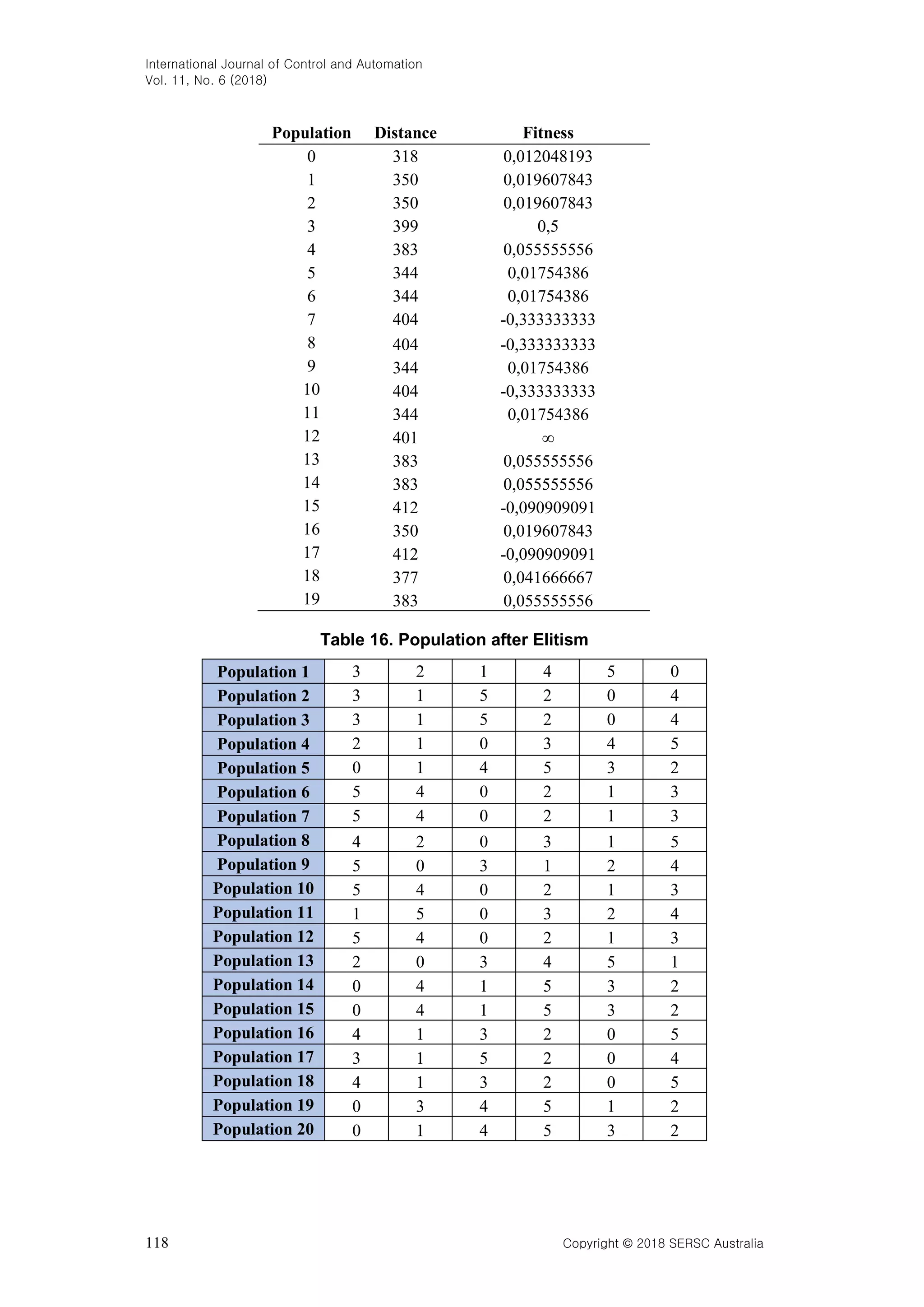
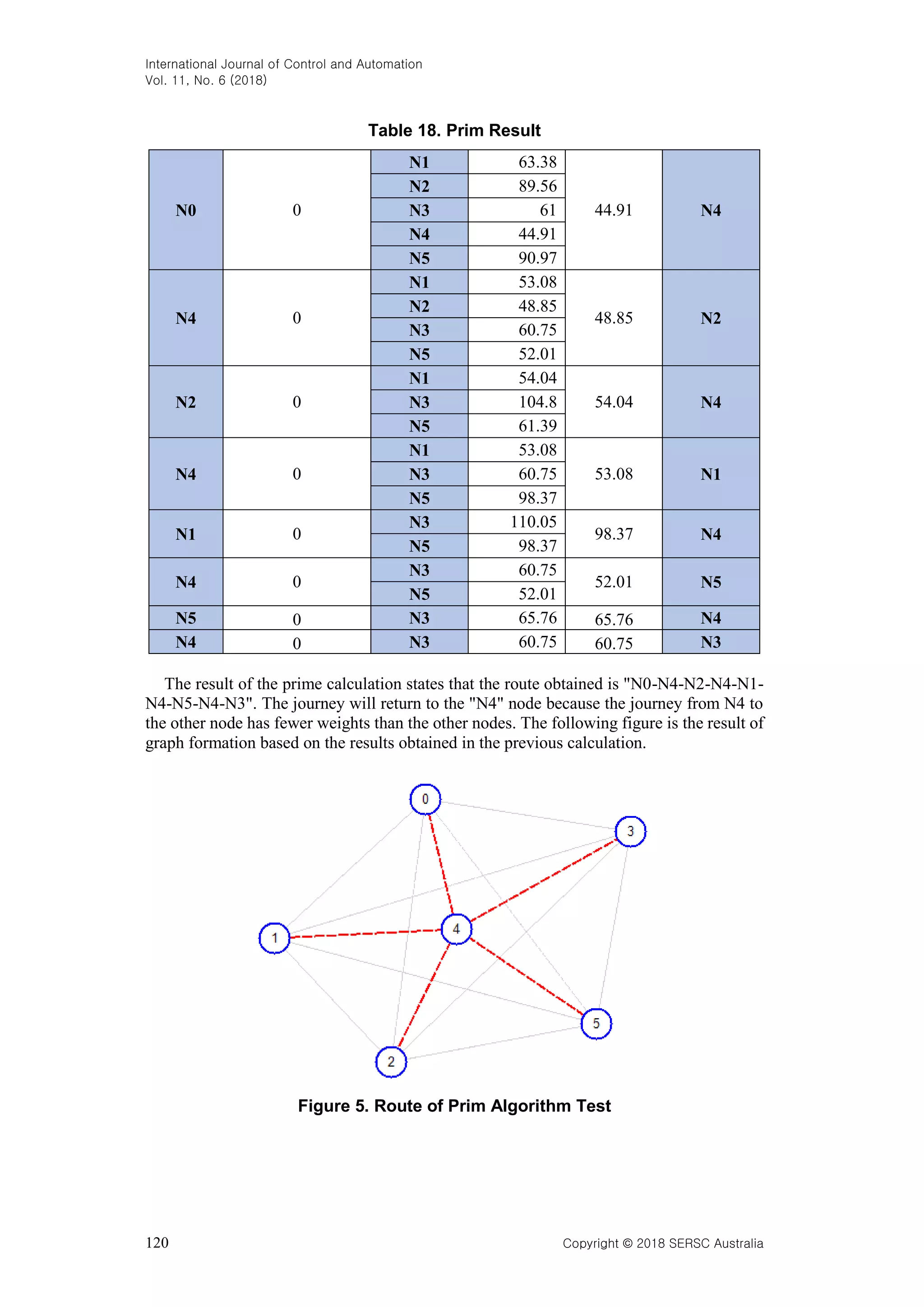
![International Journal of Control and Automation Vol. 11, No. 6 (2018) Copyright © 2018 SERSC Australia 119 The last generation shows the most optimum results for the whole generation and population. It is visible from the displayed list. Population [0] is the best value of the five populations. The route obtained is "3-2-1-4-5-0" which has a distance of 318 as shown in the following figure. Figure 4. Second Test Optimal Route After undergoing both tests, the final test result produces a more optimal value than before. In the first experiment, the optimal value obtained was 320 while in the second experiment, the optimal value increased by 2 points ie 318. This states that the more generations and populations applied to the Genetic algorithm, the better the results obtained. 3.2 Prim This algorithm works greedily. If there are several nodes as an alternative, then the selected node is the shortest node from the beginning. Table 17. Distance of each Node N0 N1 N2 N3 N4 N5 N0 0 64,38 89,56 61 44,91 90,97 N1 64,38 0 54,04 110,05 53,08 98,37 N2 89,56 54,04 0 104,8 48,85 61,39 N3 61 110,05 104,8 0 60,75 65,76 N4 44,91 53,08 48,85 60,75 0 52,01 N5 90,97 98,37 61,39 65,76 52,01 0 The following table is the result of the calculation of Prim algorithm. The trip was made from N0 to N5. At N0, five possible nodes are eligible for the next destination. Node length will be compared. It selects the shortest distance.](https://image.slidesharecdn.com/andysahputerautamasiahaan-primandgeneticalgorithmsperformanceindeterminingoptimumrouteongraph-180630063607/75/Prim-and-Genetic-Algorithms-Performance-in-Determining-Optimum-Route-on-Graph-11-2048.jpg)
![International Journal of Control and Automation Vol. 11, No. 6 (2018) Copyright © 2018 SERSC Australia 121 4. Conclusion Prim and Genetics have their respective advantages and disadvantages. Both of these algorithms aim to find the smallest weights. The use of Genetic algorithms aims to explore the entire node without returning to previously browsed nodes. Prim aims to connect the entire node based on existing connections. Both of these algorithms can work together to optimize the routes used and applied into the real world. These algorithms have a perfect role for technological advancement. References [1] S. Aryza, M. Irwanto, Z. Lubis, A. P. U. Siahaan, R. Rahim and M. Furqan, “A Novelty Design of Minimization of Electrical Losses in A Vector Controlled Induction Machine Drive”, IOP Conference Series: Materials Science and Engineering, vol. 300, (2018), no. 1. [2] M. Iqbal, A. P. U. Siahaan, N. E. Purba and D. Purwanto, “Prim’s Algorithm for Optimizing Fiber Optic Trajectory Planning”, Int. J. Sci. Res. Sci. Technol., vol. 3, no. 6, (2017), pp. 504-509. [3] A. P. U. Siahaan, “Factorization Hack of RSA Secret Numbers”. [4] V. Tasril, M. B. Ginting, Mardiana and A. P. U. Siahaan, “Threats of Computer System and its Prevention”, Int. J. Sci. Res. Sci. Technol., vol. 3, no. 6, (2017), pp. 448-451. [5] R. D. Sari, Supiyandi, A. P. U. Siahaan, M. Muttaqin and R. B. Ginting, “A Review of IP and MAC Address Filtering in Wireless Network Security”, Int. J. Sci. Res. Sci. Technol., vol. 3, no. 6, pp. 470-473, (2017). [6] D. Kurnia, H. Dafitri, M. Sugianto and A. P. U. Siahaan, “RSA 32-bit Implementation Technique”, Int. J. Recent Trends Eng. Res., vol. 3, no. 7, (2017) July, pp. 279-284. [7] A. P. U. Siahaan, “Rail Fence Cryptography in Securing Information”. [8] R. Rahim, “Searching Process with Raita Algorithm and its Application”, J. Phys. Conf. Ser., vol. 1007, no. 1, (2018), pp. 1-7. [9] A. P. U. Siahaan and R. Rahim, “Dynamic Key Matrix of Hill Cipher Using Genetic Algorithm”, Int. J. Secur. Its Appl., vol. 10, no. 8, (2016) August, pp. 173-180. [10] R. Rahim, “Combination Base64 Algorithm and EOF Technique for Steganography”, J. Phys. Conf. Ser., vol. 1007, no. 1, pp. 1-5, (2018). [11] R. F. Wijaya, Y. M. Tondang and A. P. U. Siahaan, “Take Off and Landing Prediction using Fuzzy Logic”, Int. J. Recent Trends Eng. Res., vol. 2, no. 12, (2016), pp. 127-134. [12] S. Supiyandi, M. I. Perangin-angin, A. H. Lubis, A. Ikhwan, Mesran and A. P. U. Siahaan, “Association Rules Analysis on FP-Growth Method in Predicting Sales”, Int. J. Recent Trends Eng. Res., vol. 3, no. 10, (2017), pp. 58-65. [13] M. Iswan Perangin-angin, Khairul and A. P. U. Siahaan, “Fuzzy Logic Concept in Technology, Society, and Economy Areas in Predicting Smart City”, Int. J. Recent Trends Eng. Res., vol. 2, no. 12, (2016), pp. 176-181. [14] S. Hartanto, M. Furqan, A. P. U. Siahaan and W. Fitriani, “Haversine Method in Looking for the Nearest Masjid”, Int. J. Recent Trends Eng. Res., vol. 3, no. 8, (2017) August, pp. 187-195. [15] A. P. U. Siahaan, “Genetic Algorithm in Hill Cipher Encryption”, Am. Int. J. Res. Sci. Technol. Eng. Math., vol. 15, no. 1, (2016), pp. 84-89. [16] A. P. U. Siahaan, “Adjustable Knapsack in Travelling Salesman Problem Using Genetic Process”. Int. J. Sci. Technoledge, vol. 4, no. 9, (2016), pp. 46-55. [17] A. P. U. Siahaan, “Scheduling Courses using Genetic Algorithms”, Int. J. Comput. Appl., vol. 153, no. 3, (2016), pp. 20-25. [18] I. Sumartono, D. Arisandi, A. P. U. Siahaan and Mesran, “Expert System of Catfish Disease Determinants Using Certainty Factor Method”, Int. J. Recent Trends Eng. Res., vol. 3, no. 8, (2017) August, pp. 202- 209. [19] A. P. U. Siahaan and W. Fitriani, “A Simple Comparison Between WEKA and Salford System in Data Mining Software”. [20] Z. Ramadhan, “Perbandingan Algoritma Prim dan Algoritma Floyd-Warshall dalam Menentukan Lintasan Terpendek (Shortest Path Problem)”, Universitas Sumatera Utara, (2016). [21] R. Meiyanti, A. Subandi, N. Fuqara, M. A. Budiman and A. P. U. Siahaan, “The Recognition of Female Voice Based on Voice Registers in Singing Techniques in Real-Time using Hankel Transform Method and Macdonald Function”, J. Phys. Conf. Ser., vol. 978, no. 1, (2018), pp. 1-6. [22] A. Bloomfield, “Program and Data Representation”, 2018. [Online]. Available: https://aaronbloomfield.github.io/pdr/slides/11-graphs.html?print-pdf#/cover. [Accessed: 21-May-2018]. [23] M. Iqbal, M. A. S. Pane and A. P. U. Siahaan, “SMS Encryption Using One-Time Pad Cipher”, IOSR J. Comput. Eng., vol. 18, no. 6, (2016), pp. 54-58. [24] A. P. U. Siahaan, “High Complexity Bit-Plane Security Enchancement in BPCS Steganography”, Int. J. Comput. Appl., vol. 148, no. 3, (2016), pp. 17-22.](https://image.slidesharecdn.com/andysahputerautamasiahaan-primandgeneticalgorithmsperformanceindeterminingoptimumrouteongraph-180630063607/75/Prim-and-Genetic-Algorithms-Performance-in-Determining-Optimum-Route-on-Graph-13-2048.jpg)
![International Journal of Control and Automation Vol. 11, No. 6 (2018) 122 Copyright © 2018 SERSC Australia [25] A. P. U. Siahaan, “Securing Short Message ServiceUsing Vernam Cipher in Android Operating System”, IOSR, (2016) April. [26] W. Fitriani, R. Rahim, B. Oktaviana and A. P. U. Siahaan, “Vernam Encypted Text in End of File Hiding Steganography Technique”, Int. J. Recent Trends Eng. Res., vol. 3, no. 7, (2017) July, pp. 214-219. [27] A. Q. Ansari, Ibraheem and S. Katiyar, “Comparison and analysis of solving travelling salesman problem using GA, ACO and hybrid of ACO with GA and CS”, 2015 IEEE Workshop on Computational Intelligence: Theories, Applications and Future Directions (WCI), (2015), pp. 1-5. [28] Z. Sitorus and A. P. U. Siahaan, “Heuristic Programming in Scheduling Problem Using A* Algorithm”, IOSR J. Comput. Eng., vol. 18, no. 5, (2016), pp. 71-79. [29] A. P. U. Siahaan, “Heuristic Function Influence to the Global Optimum Value in Shortest Path Problem”, IOSR J. Comput. Eng., vol. 18, no. 05, (2016) May, pp. 39-48. [30] A. P. U. Siahaan, “Determination of Thesis Preceptor and Examiner Based on Specification of Teaching Using Fuzzy Logic”. [31] Z. Tharo and A. P. U. Siahaan, “Profile Matching in Solving Rank Problem”, IOSR J. Electron. Commun. Eng., vol. 11, no. 05, (2016) May, pp. 73-76. [32] H. A. Hasibuan, R. B. Purba and A. P. U. Siahaan, “Productivity Assessment (Performance, Motivation, and Job Training) using Profile Matching”, Int. J. Econ. Manag. Stud., vol. 3, no. 6, (2016), pp. 73-77.](https://image.slidesharecdn.com/andysahputerautamasiahaan-primandgeneticalgorithmsperformanceindeterminingoptimumrouteongraph-180630063607/75/Prim-and-Genetic-Algorithms-Performance-in-Determining-Optimum-Route-on-Graph-14-2048.jpg)

The document analyzes the performance of Prim's and Genetic algorithms in finding optimal routes on a graph, focusing on speed, efficiency, and suitability for various problems like the minimum spanning tree and traveling salesman problem. Prim's algorithm is noted to be faster and more effective for larger vertex counts, while Genetic algorithms have strengths in handling probabilities and multiple generations, albeit at the cost of increased computation time. The research also includes experimental results comparing various optimization techniques, highlighting the potential of hybrid approaches.