Download to read offline
![Send Orders for Reprints to reprints@benthamscience.net Recent Advances in Electrical and Electronic Engineering, 2019, Volume, Page Enation 1 xxxx-xxxx /19 $58.00+.00 © 2019 Bentham Science Publishers ARTICLE TYPE Title: Short Term Load Forecasting Using Bootstrap Aggregating Based Ensemble Artificial Neural Network Muhammad Faizan Tahira , Chen Haoyong*a , Kashif Mehmoodb , Nauman Ali Laraika and Saif ullah Adnana , Khalid Mehmood Cheemab a School of Electric Power, South China University of Technology, Guangzhou, China; b School of Electrical Engineering, Southeast University, Nanjing, China Abstract: Short Term Load Forecasting (STLF) can predict load from several minutes to week plays the vital role to address challenges such as optimal generation, economic scheduling, dispatching and contingency analysis. This paper uses Multi-Layer Perceptron (MLP) Artificial Neural Network (ANN) technique to perform STFL but long training time and convergence issues caused by bias, variance and less generalization ability, unable this algorithm to accurately predict future loads. This issue can be resolved by various methods of Bootstraps Aggregating (Bagging) (like disjoint partitions, small bags, replica small bags and disjoint bags) which helps in reducing variance and increasing generalization ability of ANN. Moreover, it results in reducing error in the learning process of ANN. Disjoint partition proves to be the most accurate Bagging method and combining outputs of this method by taking mean improves the overall performance. This method of combining several predictors known as Ensemble Artificial Neural Network (EANN) outperform the ANN and Bagging method by further increasing the generalization ability and STLF accuracy. A R T I C L E H I S T O R Y Received: Revised: Accepted: DOI: Keywords: Short term load forecasting, Artificial neural network, Multi-layer perceptron, Bootstrap aggregating, Disjoint partition, Ensemble artificial neural network 1. INTRODUCTION Rapid growth in electricity demand increasing the need for attaining secure and economic network to fulfil users demand at all-time while considering economic constraints [1, 2]. Optimal power flow and electric power quality are fundamental features of sustainable economic activities and this can be achieved by load forecasting [3, 4]. Load forecasting determines the load behaviour that helps in predicting the amount of power required to meet the demand [5, 6]. In this way, it helps to acquire a secure, optimal and fault-less power system network. Load forecasting is divided into Short Term Load Forecasting (STLF), medium term and long term load forecasting [7] but this research is limited to STLF that starts from minutes to week anticipation [8, 9]. STLF is employed for on-line generation scheduling, power system security evaluation, saving start-up and investment costs [10, 11]. In addition, proper scheduling maintains system stability and also prevents cascaded failure [6, 12]. Weather parameters, customers’ types, time factors and some random factors influence the STLF variable [13, 14]. Weather data considered weather characteristics for peak historical load and it usually varies over a period of 25-30 years. Seasonal effects either weekly or daily cycle or the government announced holidays are the prominent time factors that influence load patterns. System load comprises of diverse individual power demands and every user subject to some random disturbances such as industrial facilities shut down, widespread spikes and so on. Its effect on the system is uncertain that is why these factors lie under the category of random factors. STLF has been carried out for a long time and many scholars have done comprehensive research and propose various prediction models using different algorithms. Classical prediction techniques such as nonparametric regression [15], time series method [16], grey prediction methods [17] and computational intelligence techniques like Artificial Neural Network (ANN) [18], Particle Swarm Optimization (PSO) [19]](https://image.slidesharecdn.com/jraeeshorttermloadforecastingusingbootstrapaggregatingbased-200420214532/75/Short-Term-Load-Forecasting-Using-Bootstrap-Aggregating-Based-Ensemble-Artificial-Neural-Network-1-2048.jpg)
![2 Journal Name, 2019, Vol. 0, No. 0 M.F. Tahir et al. and Genetic Algorithm (GA) [20] and many others have been used in past to address this issue. ANN is preferred among other intelligence techniques due to its aptness to self-learn and perform well for complex non-linear problems. However, these days hybridization of various techniques with ANN to solve STLF is getting more attention and few of these techniques are listed in Table I. TABLE I DIFFERENT HYBRID TECHNIQUES USED FOR STLF HYBRIDIZATION ADVANTAGES OVER UN-HYBRID ANN ANN TYPE ANN - Artificial Immune System (AIS) [21] High accuracy and fast convergence and improved Mean Average Percentage Error (MAPE) Feed Forward Back Propagation (FFBP) ANN ANN - Fuzzy [22] Improvement in prediction accuracy and reduction in forecasting error Levenberg-Marquardt Back Propagation (LMBP) ANN ANN - GA [23] Better performance and good ability of solving the problem FFBP ANN ANN - PSO [24] More accurate Radial Basis Function (RBF) ANN ANN - CPSO [25] Improves searching efficiency and quality RBF ANN ANN - firefly [26] Improves both local and global searching ability FFBP ANN ANN – Support Vector Machine (SVM) [27] Better forecasting accuracy and high speed FFBP ANN Aforementioned hybridization techniques achieve better results than ANN because ANN suffers from noise, bias, variance and inefficient generalization ability. However, if these problems can be resolved then ANN will be able to achieve improved results in less computational time than hybridization techniques. Main contributions of this work are: i) ANN is trained for three years (2007-2009) data to calculate 2010 data that is taken from Australian Market. Humidity, system load, wet bulb, dew point and dry bulb temperature acts as inputs while 2010 data acts as target output for the ANN network. ii) ANN inability to accurately predict 2010 forecasted data is improved by 4 Bootstrap Aggregating (Bagging) algorithms that just resample the original data which will help in increasing generalization ability and reducing variance. iii) Disjoint partition proves to be superior than other three Bagging methods and Ensemble Artificial Neural Network (EANN) combines the output of this method to increase accuracy further. Rest of the paper is organized as follows: Section 2 briefly elaborates ANN, Bagging and EANN techniques while section 3 discusses methodology and data used for ANN training. Section 4 illustrates results simulation and section 5 concludes the paper. 2. ANN, BAGGING AND EANN 2.1. Artificial neural network The basic idea of ANN derives from the biological nervous system [28, 29]. The key element for processing information in the neural network is neuron. A Neuron has four main parts and these elements form the basic building block for ANN as shown in Fig. 1. Fig. 1. Biological and ANN architecture ANN output from output function is compared with the desired results and in the case of mismatching both outputs indicates there is some error. Some architecture utilizes this error directly while some squares it or cube it to modify according to the specific purpose. The error is propagated backwards to adjust the weights of input so that desired output matches the ANN output. This adjustment of weight and backward propagation of error accounts in the learning function in which some specified algorithm is used for this function to minimize the error. Four performance metrics like Mean Square Error (MSE), Root Mean Square Error (RMSE), Mean Absolute Percentage Error (MAPE) and Mean Absolute Deviation (MAD) are used in this work for reduction in the learning process as indicated in equations 1- x1 xn x2 . . Dendrites Soma Axon Synapses Input function Weighting factors Transfer function Output function w1j w2j w3j Σ ψ Activation function](https://image.slidesharecdn.com/jraeeshorttermloadforecastingusingbootstrapaggregatingbased-200420214532/75/Short-Term-Load-Forecasting-Using-Bootstrap-Aggregating-Based-Ensemble-Artificial-Neural-Network-2-2048.jpg)
![Title of the Article Recent Advances in Electrical and Electronic Engineering, 2019, Vol. 0, No. 0 3 4. 2 2 1 1 1 1 ( ) ( ) n n i i i i MSE e i t y n n (1) 2 2 1 1 1 1 ( ) ( ) n n i i i i RMSE e i t y n n (2) 1 1 n i i i MAD t y n (3) 1 1 100 n i i i i t y MAPE n t (4) where, n is number of examples, i represents iterations, it is desired target value and iy is ANN output value. ANN does not need to be programmed, it just learns that causes it to work well with large data sets and complex non-linear problems. Moreover, it easily solves the problems that are difficult to specify it mathematically and do not have particular knowledge about the problem. However, sometimes it cannot extrapolate desired results even after trying different training algorithms, activation functions and structures. This difficulty in extrapolating desired results can be due to an error in the learning process that occurs due to noise, bias and variance. Bias and Variance cause underfitting and overfitting of data respectively due to ANN inability to learn target function and fluctuations in training dataset. 2.2. Bootstrap aggregating Bootstrap Aggregating commonly known as Bagging was presented by Breiman [30] that helps in minimizing the variance by reducing the overfitting which increases the precision of machine learning algorithms [31]. Disjoint partition, small bags, no replication small bags and disjoint bags are common methods of Bagging which are elaborated in by considering the below hypothetical dataset shown in Fig. 2(a). Fig. 2(a). Hypothetical data set The disjoint partition divides the data in small subsets into such a pattern that set union of subsets must be equal to hypothetical data set and each classifier is selected by once. In contrary, subsets created by small bags may not necessarily be equal to the above data because of repetition of few classifiers and in no replication small bags method, no repetition occurs while generating subset independently but still the union of subsets may not be equal to above data. Disjoints bags training is carried out in a similar fashion to disjoint bags but it is the only method in which there is the possibility of increasing the subset size than original size as depicted in Figs. 2 (b-e). Fig. 2(b). Disjoint partition Fig. 2(c). Small bags Fig. 2(d). No replication small bags Fig. 2(e). Disjoint bags Bagging not only minimizes variance but this random distribution of data increases the generalization ability of neural networks. Therefore, the creation of multiple Bootstraps and again training ANN improves the overall accuracy. C. Ensemble artificial neural network EANN is a method of combining different ANN outputs and obtaining one single output [32, 33]. This process can be summed up as sketched in Fig. 3 Fig. 3. Ensemble artificial neural network A B C D E F G H I J K L M N O P A B C D M N O PI J K LE F G H A C D E D P E F I A K H M O J L A C H LO P L N D I O H K C F P A B C D B E F G H G I J K L I M N O P N Training the bootstraps again and chooses the best bootstrap method for EANN ANN Model B1 BNB2 EANN Model It suffers with variance and bias Creation of multiple bootstraps increases the ANN generalization ability Combining multiple outputs increases the accuracy . . . . Final accurate EANN output B1 B2 BN. . . .](https://image.slidesharecdn.com/jraeeshorttermloadforecastingusingbootstrapaggregatingbased-200420214532/75/Short-Term-Load-Forecasting-Using-Bootstrap-Aggregating-Based-Ensemble-Artificial-Neural-Network-3-2048.jpg)
![4 Journal Name, 2019, Vol. 0, No. 0 M.F. Tahir et al. Combination of several predictors outweighs the prediction of individual predictors [12]. Therefore, EANN which combines multiple outputs as shown above guarantees a reduction in error and improvement in accuracy. Moreover, generalization ability and performance of the whole system increases significantly that has been shown in the results section. 3. METHODOLOGY AND DATA COLLECTION The data is taken from the Australian market as follows Temperature data from Bureau of Meteorology (BOM) [34]. Load data from Australian Energy Market Operator (AEMO) [35]. The data for the year 2007, 2008 and 2009 comprises of quantities mentioned in table II but for the sake of simplicity only data of first 12 hours of January 2007 is depicted in this work. TABLE II DATA FOR ANN LOAD FORECASTING Given Data Date Time (hour) Dry Bulb (Celsius o C) Dew Point (Celsius o C) Wet Bulb (Celsius o C) Humidity (g/kg) System Load (MW) 1-Jan-2007 0.0 20.40 15.2 17.30 72.0 7228.86 1-Jan-2007 0.5 20.35 15.3 17.35 72.5 7062.49 1-Jan-2007 1.0 20.30 15.4 17.40 73.0 6843.66 1-Jan-2007 1.5 20.25 15.5 17.45 74.0 6552.34 1-Jan-2007 2.0 20.20 15.7 17.50 75.0 6296.34 1-Jan-2007 2.5 20.15 15.9 17.60 76.5 6079.49 1-Jan-2007 3.0 20.10 16.1 17.70 78.0 5957.18 1-Jan-2007 3.5 20.10 15.8 17.55 76.5 5913.07 1-Jan-2007 4.0 20.10 15.6 17.40 75.0 5855.45 1-Jan-2007 4.5 19.75 16.3 17.65 80.5 5884.93 1-Jan-2007 5.0 19.40 17.0 17.90 86.0 5904.63 1-Jan-2007 5.5 19.90 16.4 17.80 80.5 5953.51 1-Jan-2007 6.0 20.40 15.9 17.70 75.0 6040.14 1-Jan-2007 6.5 20.65 15.9 17.80 74.0 6150.36 1-Jan-2007 7.0 20.90 15.9 17.90 73.0 6332.48 1-Jan-2007 7.5 20.60 16.5 18.15 77.5 6577.33 1-Jan-2007 8.0 20.30 17.1 18.40 82.0 6796.30 1-Jan-2007 8.5 20.10 16.85 18.15 81.5 7015.00 1-Jan-2007 9.0 19.90 16.6 17.90 81.0 7250.31 1-Jan-2007 9.5 20.05 17.3 18.35 84.0 7470.74 1-Jan-2007 10 20.20 17.9 18.80 86.7 7574.95 1-Jan-2007 10.5 21.40 16.8 18.60 76.0 7666.11 1-Jan-2007 11.0 22.60 15.6 18.40 65.0 7762.30 1-Jan-2007 11.5 22.50 15.2 18.15 63.5 7758.87 1-Jan-2007 12.0 22.40 14.8 17.90 62.0 7750.38 3.1. Initialization, training and adaptation of ANN Load of any electric unit is comprised of various consumption units (industrial, commercial and residential) and different factors (like meteorological](https://image.slidesharecdn.com/jraeeshorttermloadforecastingusingbootstrapaggregatingbased-200420214532/75/Short-Term-Load-Forecasting-Using-Bootstrap-Aggregating-Based-Ensemble-Artificial-Neural-Network-4-2048.jpg)
![Title of the Article Recent Advances in Electrical and Electronic Engineering, 2019, Vol. 0, No. 0 5 conditions, economic and demographic factors, time factors and other random factors) affect the electric load depending on the specific consumption unit. Generally, load forecasting is categorized into three periods: Long, medium and short terms. This research is focused on short term load forecasting which is mostly based on climate conditions like dry bulb temperature, wet bulb temperature, humidity and dew point temperature [36]. Therefore, above six inputs are used as inputs for modelling neural network to determine the desired load. Multi-Layer Perceptron neural network model are chosen because they are comparatively simpler to implement and have several applications in case of nonlinear mapping among inputs and outputs such as behavioral modelling, adaptive control and image recognition and so on []. Moreover, Levenberg- Marquardt training is used because it is the fastest backpropagation algorithm in the nntool box which is recommended as a first choice for supervised learning algorithm []. Above parameters of three years data (2007-2009) act as inputs and after normalizing input datasets, it is used for ANN training to forecast 2010 data and then compared with actual 2010 data which serve as targeted output has been made. ANN output and targeted outputs are not 100 percent accurate that shows areas of improvement which is accomplished by Bagging and EANN. MATLAB provides nntool for ANN creation, input data, target data, network type, training function and other parameters required for ANN training are summarized in table III. TABLE III ANN PARAMETERS DETAILS Parameters Details Number of input neurons 6 (time, dry bulb, dew point and wet bulb temp, humidity and system load) Number of output neurons 1 (forecasted data) Number of hidden-layer neurons 20 Neural network model Multi-Layer Perceptron Training function Levenberg-Marquardt Back Propagation Adaptation learning function Gradient descent with momentum weight and bias Number of layers 2 Activation function for layer 1 Trans sigmoid Activation function for layer 2 Pure linear Performance function MAD, MSE, RMSE, MAPE Percentage of using information Train (70%), test (15%), cross validation (15%) Maximum of epoch 1000 Learning rate 0.01 Maximum validation failures 6 Error threshold 0.001 Weight update method Batch](https://image.slidesharecdn.com/jraeeshorttermloadforecastingusingbootstrapaggregatingbased-200420214532/75/Short-Term-Load-Forecasting-Using-Bootstrap-Aggregating-Based-Ensemble-Artificial-Neural-Network-5-2048.jpg)
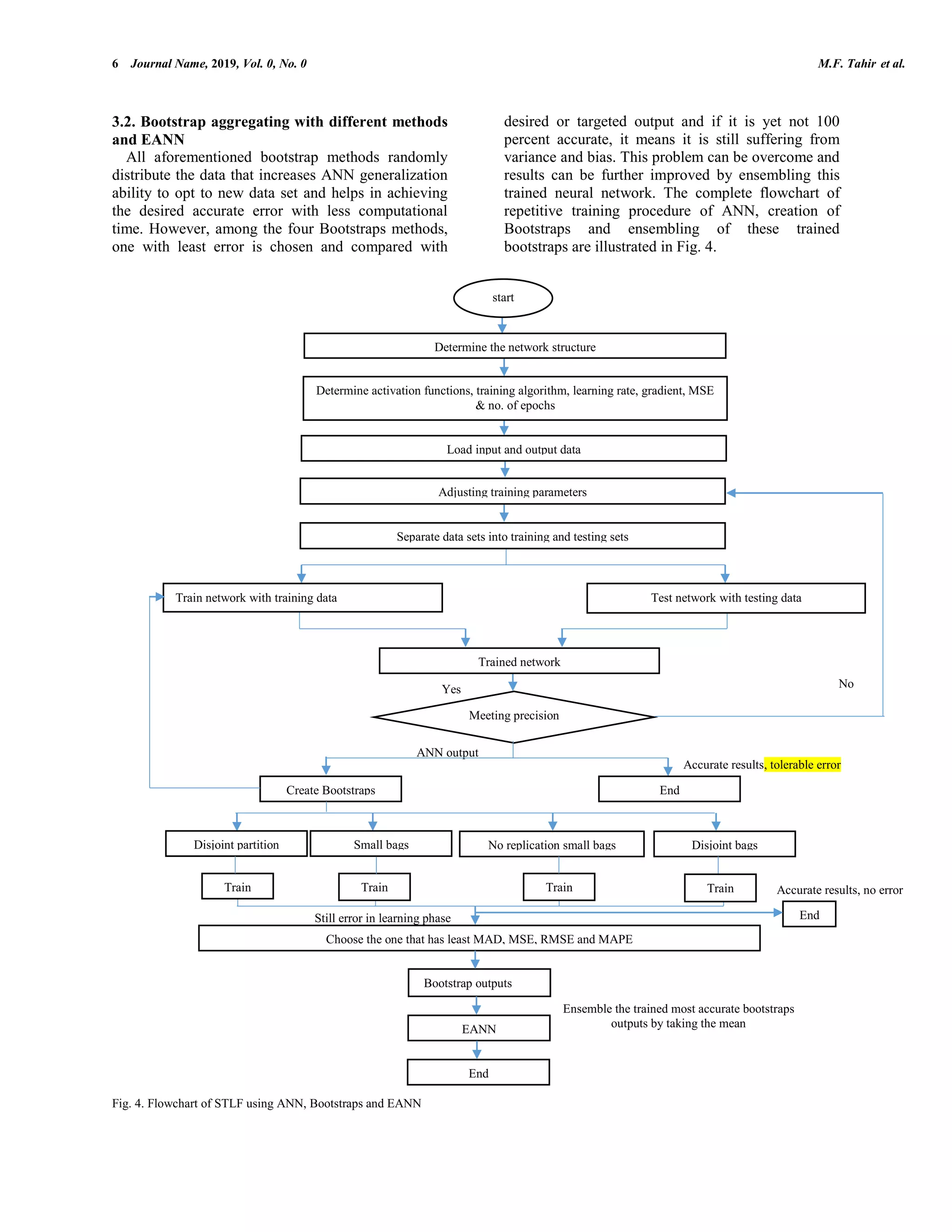


The document discusses a research paper focused on short-term load forecasting (STLF) using a bootstrapped ensemble of artificial neural networks (ANN). It highlights the challenges faced by traditional ANN in predicting future loads due to issues like long training times and convergence problems, which are resolved through techniques like bootstrap aggregating and ensemble methods. The study demonstrates that combining outputs from disjoint partitions leads to improved accuracy and generalization ability in STLF predictions.