Downloaded 10 times
![International Journal in Foundations of Computer Science & Technology (IJFCST) Vol.5, No.5, September 2015 DOI:10.5121/ijfcst.2015.5502 9 MULTI-HOP DISTRIBUTED ENERGY EFFICIENT HIERARCHICAL CLUSTERING SCHEME FOR HETEROGENEOUS WIRELESS SENSOR NETWORKS Sheenam M. Tech Research Scholar Department of Electronics and communication Engineering, Punjabi University, Patiala, India ABSTRACT Wireless sensor network (WSNs) are network of Sensor Nodes (SNs) with inherent sensing, processing and communicating abilities. One of current concerns in wireless sensor networks is developing a stable clustered heterogeneous protocol prolonging the network lifetime with minimum consumption of battery power. In the recent times, many routing protocols have been proposed increasing the network lifetime, stability in short proposing a reliable and robust routing protocol. In this paper we study the impact of hierarchical clustered network with sensor nodes of two-level heterogeneity. The main approach in this research is to develop an enhanced multi-hop DEEC routing protocol unlike DEEC. Simulation results show the proposed protocol is better than DEEC in terms of FDN (First Dead Node), energy consumption and Packet transmission. KEYWORDS Wireless Sensor Networks, FDN, DEEC, Heterogeneity, Intermediate Nodes, Network Lifetime. 1. INTRODUCTION Wireless sensor networks are composed of thousands or more sensor nodes which are distributed manually or randomly in physical sensor environment to sense the characteristics of environment. The main aim behind such deployment is to fulfill some particular aim of particular application such as acoustics, temperature, humidity, light, seismic etc [1]. Network collect the environment data and forward to processing nodes for further processing. These nodes in high density are deployed in buildings, homes, highways, cities [2]. The range of applications is from warning natural disasters, protecting homeland, conducting surveillance, wildlife monitoring, environment monitoring etc. These sensor nodes are considered as energy scarce system resources as they have short battery life [3]. The cost is more in transmission of data than processing of data so if there can be a scheme where this transmission distance is decreased with some sort of changes in deployment, it would be a boon for the system. In Direct transmission (DT), the data from sensor nodes (SNs) is transmitted directly to BS (Base Station). In such transmission if the Bs is located far away from SNs, the sensor nodes away would require more energy than nearby sensor nodes in DT. Similarly in MTE (Minimum Transmission Energy), sensor nodes are sending data to neighboring sensor nodes and finally](https://image.slidesharecdn.com/5515ijfcst02-151009101938-lva1-app6892/75/MULTI-HOP-DISTRIBUTED-ENERGY-EFFICIENT-HIERARCHICAL-CLUSTERING-SCHEME-FOR-HETEROGENEOUS-WIRELESS-SENSOR-NETWORKS-1-2048.jpg)
![International Journal in Foundations of Computer Science & Technology (IJFCST) Vol.5, No.5, September 2015 10 reach BS, here the nodes near to BS are more participating in data transmission than faraway nodes, so they are draining their energy faster and die faster as compared to other nodes [4]. Even there is no resource for recharging of sensor nodes after particular time period if they are not been installed with energy recharging resources. So maximizing the network lifetime with energy efficiency is current challenge that we are facing in this field. Clustering [2] is a technique used for reducing energy usage by assigning a Cluster Head (CH) for aggregating data and forwarding this aggregated data to BS. CH here is acting as intermediate node between sensor nodes and BS. Flat network is network of sensor nodes with no CH and no cluster formation and each sensor node is sending its data to other node or to BS but clustered network is network of clusters with one CH of each cluster for data transmission as shown in figure 1[5]. In Clustered network, the whole network is composed of group of sensor nodes called as cluster with one head of family (cluster) who is responsible for data communication with other BS. Figure 1. Network operations of WSNs Even after clustering still wireless sensor networks are suffering from un-efficient energy management. So in this research we are proposing a large scale multi-hop network system infrastructure comprising of sensor nodes having low battery power and processing, computing capabilities. Intermediate rechargeable nodes are deployed in network field for enhancing the lifetime of networks. Intermediate nodes so placed are decreasing the average distance of data transmission form sensor nodes to BS. 2. RELATED WORK LEACH [4] was first clustered homogeneous network scheme which uses direct transmission of data from CH selected randomly to BS leads to draining of energy of sensor nodes quickly. Prior selecting is not done as it may lead to some unfavorable nodes becoming CHs that would die Internet and satellite User Task/ Manager Node Sensor node Cluster Head Flat network Clustered Network](https://image.slidesharecdn.com/5515ijfcst02-151009101938-lva1-app6892/75/MULTI-HOP-DISTRIBUTED-ENERGY-EFFICIENT-HIERARCHICAL-CLUSTERING-SCHEME-FOR-HETEROGENEOUS-WIRELESS-SENSOR-NETWORKS-2-2048.jpg)
![International Journal in Foundations of Computer Science & Technology (IJFCST) Vol.5, No.5, September 2015 11 quickly. LEACH outperforms DT and MTE in terms of network stability. PEGASIS [6] was a chain based routing scheme provides improvement over LEACH scheme. Each node communicates with nearby node and take turns of transmission until reaches BS. PEGASIS was twice better than LEACH in terms of network lifetime. HEED [7] was proposed as an enhancement over homogeneous protocols like LEACH, PEGASIS, TEEN etc where CH was selected based on node residual energy and also on basis of node proximity to nearby node i.e. node’s degree. HEED outperforms other routing protocols. All the above protocols described are homogeneous considering each node of similar architecture, computing capabilities and initial energy. But then comes the SEP [8] where discrimination in nodes in terms of energy is considered i.e. higher energy nodes are advance nodes and low energy nodes are normal nodes. CH is chosen based on initial energy of nodes. SEP outperforms the other protocols like LEACH in terms of network stability. DEEC [9] is also a heterogeneous clustered routing protocol where CHs are chosen based on node’s residual energy and DEEC outperforms SEP in terms of stability. DDEEC [10] is another advancement of DEEC which permits to balance the CH selection over the whole network based on residual energy. H-SEP [11] (Heterogeneous SEP) is an advancement over SEP introducing two level heterogeneity in terms of node energy. H-SEP outperforms SEP in terms of lifetime. SEP-E [12] (Enhanced SEP) was proposed as an advancement of SEP where three-level heterogeneity is been considered. Three types of nodes with different energy levels is been taken. SEP-E outperforms LEACH and SEP in terms of FDN and throughput. HSEP [13] is a heterogeneity aware hierarchical stable election protocol which tends to increase the lifetime of WSNs by choosing two types of CHs i.e. primary and secondary CHs. Primary CH are taken from secondary ones. HSEP outperforms SEP, LEACH, DEEC by 75%, 61%, 52% resp. M-GEAR [14] for WSNs introduced gateway node at center of network and BS out of field. Simulation results showed M-GEAR outperforms LEACH in terms of network lifetime, throughput etc. ZSEP [15] uses both the direct transmission and clustering. ZSEP divide the sensor network in three zones depending on distance from BS. ZSEP outperforms SEP in terms of stability of network. MDEEC [16] modifies the existing DEEC allowing more number of data to be transferred to BS in particular time interval. Simulation results showed MDEEC has incremented message transmission when compared to existing LEACH and DEEC protocol. SEARCH [17] was proposed to increase the number of half alive nodes and stability. SEARCH (Stochastic election of appropriate range cluster heads) updates the G value quickly making the availability of nodes all the time for becoming CHs. 3. PROPOSED DEEC (IDEEC PROTOCOL) The basic assumptions of new proposed IDEEC model are as: 1. The BS is kept at 35m distance away from 100m*100m sensor network field. 2.16 intermediate nodes are placed inside the network field in a proper manner. 3. Intermediate nodes so placed are rechargeable. 4. Each sensor node is equipped with GPS to make them location aware. 5. BS also is aware of its position in field and position of sensor nodes. 6. Distance to be covered for transmission is reduced with aid of these intermediate nodes. 7. Each Sensor node is equipped with one distinct location ID.](https://image.slidesharecdn.com/5515ijfcst02-151009101938-lva1-app6892/75/MULTI-HOP-DISTRIBUTED-ENERGY-EFFICIENT-HIERARCHICAL-CLUSTERING-SCHEME-FOR-HETEROGENEOUS-WIRELESS-SENSOR-NETWORKS-3-2048.jpg)
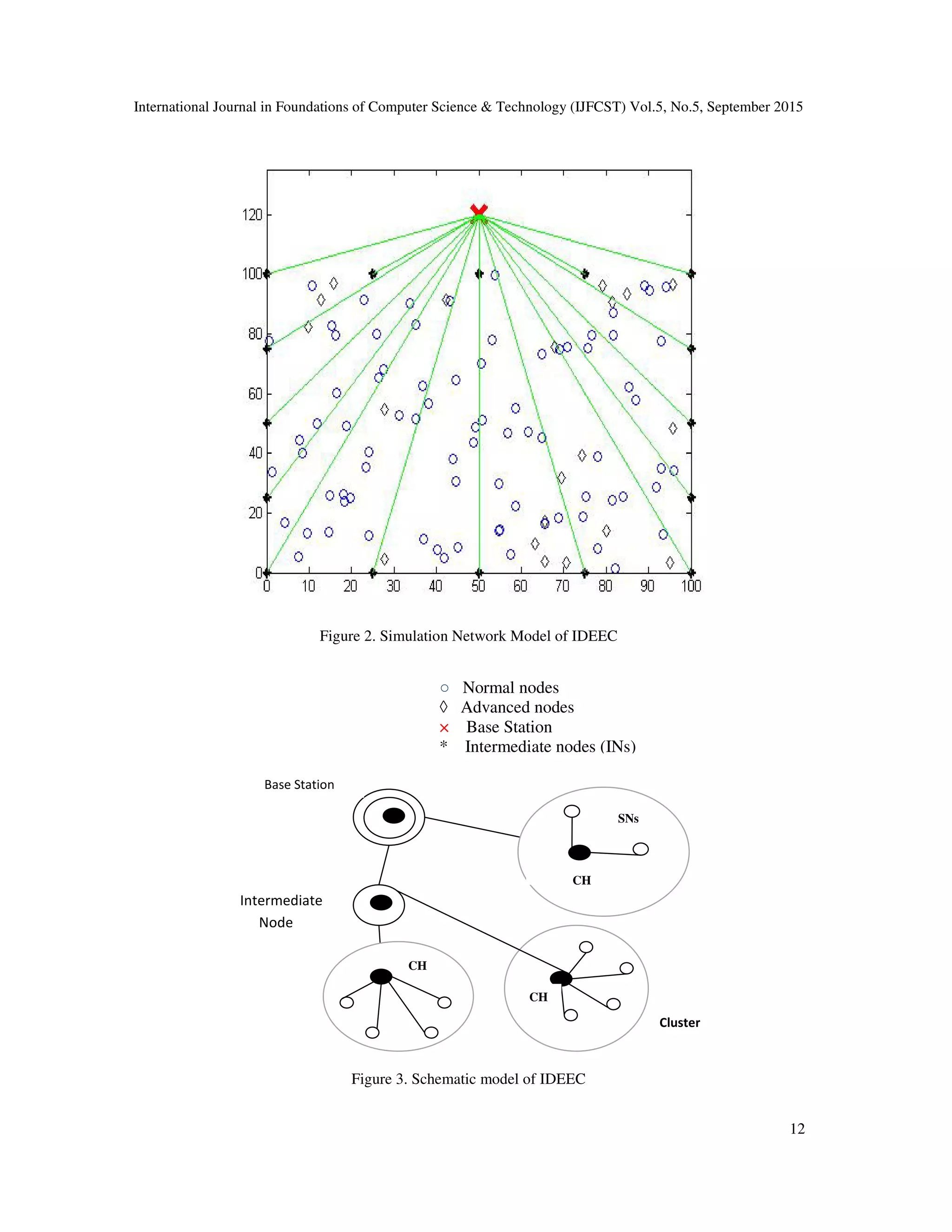
![International Journal in Foundations of Computer Science & Technology (IJFCST) Vol.5, No.5, September 2015 13 Here in this research a large scale multi-hop network system we consider four types of sensor nodes i.e. Normal Nodes, Advance Nodes and Intermediate Nodes (INs) and final Base Station (BS) Node shown in figure 3. Normal nodes and advance nodes are having limited battery power and are non-rechargeable whereas the Intermediate nodes are rechargeable and have unlimited battery power. More over the BS so placed is stationary as well as rechargeable. Sensor nodes form clusters and send data to their CH. CH discovers the nearby intermediate node and forward data to BS. The number of intermediate nodes placed at four boundaries of network field so the data out of field has to go through these intermediate nodes and then to BS. One intermediate node is receiving data from one CH data time and incase of failure of one intermediate node, data can be forwarded from another intermediate node. The main function of intermediate node (INs) is to collect data from CHs and forward that aggregated data to BS. Here we used radio propagation model as data is transmitted through Radio, infra-red or optical media in wireless sensor networks. This model was proposed in LEACH and SEP [4, 7] shown in figure 4. The energy expended by radio in achieving minimum SNR level in transmitting 4000 bits long packet bits from transmitter to receiver is given as , = . + ∈ . , ≤ . + ∈ . , > (1) Where, is the energy dissipated per bit to run the transmitter or the receiver circuit, ∈ and ∈ depends on the transmitter amplifier model, and d is the distance between the sender and the receiver. Figure 4. Radio dissipation model Model considers transmitter, amplifier and receiver. L-bit data is been transmitted from sender to receiver. do is threshold distance between two communicating ends. At d=do = ∈ ! ∈"# (2) Transmitter TX Amplifier Receiver L- bit E%& (l, d) E'('). L ∈. Ld, E-. L E'('). L L-bit d](https://image.slidesharecdn.com/5515ijfcst02-151009101938-lva1-app6892/75/MULTI-HOP-DISTRIBUTED-ENERGY-EFFICIENT-HIERARCHICAL-CLUSTERING-SCHEME-FOR-HETEROGENEOUS-WIRELESS-SENSOR-NETWORKS-5-2048.jpg)
![International Journal in Foundations of Computer Science & Technology (IJFCST) Vol.5, No.5, September 2015 14 4. CH SELECTION ALGORITHM OF IDEEC In this research multi-hop DEEC using INs is proposed. The cluster head of each cluster is selected on basis of ratio of residual energy to average energy [8]. Different probability of CH selection is their i.e. for normal nodes and advance nodes. Selection of INs is done based on distance from selected CH. Even the sensor nodes can send data directly to BS if their distance from BS is less than CH or IN. Also CH can send data directly to BS if their distance from BS is less than from IN. Average energy is ideal energy that each node shown to make system alive for longer time. Average energy is given as E/ = 0 1 ∑ E3 1 340 (3) Where E3 is residual energy of each sensor node. N is number of sensor nodes deployed. The weighted election probability of normal nodes p678 and advance nodes p/9, is given as p678 = :;<= 0>80×@0 × AB AC (4) p/9, = :;<= 0>80×/0 × 1 + a1 × AB AC (5) where m1 is fraction of advance nodes having α1% extra energy in comparison to m fraction of advance nodes with α % additional energy in DEEC [8]. pG:H is the optimal probability assumed in priori. After selecting the CHs from each processing round, a random number is generated based on which the CH is chosen from those selected CHs. After generating the random number it is compared with threshold value accordingly the CH is chosen if the number is less than threshold value. Threshold value for normal nodes T n678 and advance nodes T n/9, given as T n678 = K :LMN 0O:LMNP7 ×8G9 Q R <LMN ST , if n ∈ g′ 0 otherwise a (6) T n/9, = K :Cbc 0O:Cbcd7 ×8G9 e R <Cbc fg , if n ∈ g′′ 0 otherwise a (7) Sensor nodes with more residual energy have more chances to become CH than other nodes.](https://image.slidesharecdn.com/5515ijfcst02-151009101938-lva1-app6892/75/MULTI-HOP-DISTRIBUTED-ENERGY-EFFICIENT-HIERARCHICAL-CLUSTERING-SCHEME-FOR-HETEROGENEOUS-WIRELESS-SENSOR-NETWORKS-6-2048.jpg)

![International Journal in Foundations of Computer Science & Technology (IJFCST) Vol.5, No.5, September 2015 25 6. CONCLUSIONS In this research a new protocol is proposed named IDEEC using intermediate nodes between CHs and BS. The number of half dead nodes, alive nodes, and dead nodes showed 28%, 38%, 38% improvement respectively. FND showed improvement of 13.8 % and 18% improvement in residual energy. The lifetime of network increased by 34.66% on an average of three parameters i.e. half dead nodes, dead nodes and alive nodes. The BS is placed out of network field and rechargeable intermediate nodes inside the field with other nodes. REFERENCES [1] N. Rahmani, H. Kousha, L. Darougaran, and F. Nematy, (2010) " CAT: The New Clustering Algorithm Based on Two-Tier Network Topology for Energy Balancing in Wireless Sensor Networks," in International Conference on Computational Intelligence and Communication Networks (CICN), pp. 275-278. [2] W. B. Heinzelman, A. P. Chandrakasan, and H. Balakrishnan, (2002) "An application-specific protocol architecture for wireless microsensor networks," Wireless Communications, IEEE Transactions on, vol. 1, pp. 660-670. [3] L. Dehni, F. Krief, and Y. Bennani, (2006) "Power Control and Clustering in Wireless Sensor Networks," in Challenges in Ad Hoc Networking. vol. 197, pp. 31-40. [4] W.R. Heinzelman, A. Chandrakasan and H. Balakrishnan, (2000) “Energy-efficient communication protocol for wireless microsensor networks”, In Proc. International Conference on System Sciences, pp. 4-7, Maui, Hawaii. [5] Q. Wang and I. Balasingham, (2010) “Wireless sensor networks: Application centric design”, Journal of Communications, vol. 2, no. 5, pp. 134-149. [6] S. Lindsey and C.S. Raghavendra, (2002) “PEGASIS: Power-Efficient Gathering in Sensor Information Systems”, IEEE Proceedings on Aerospace, vol. 3, no.2, pp.1-6. [7] O. Younis and S. Fahmy, (2004) "HEED: A hybrid, energy efficient, distributed clustering approach for ad hoc sensor networks", IEEE Transactions on Mobile Computing, vol. 3, no. 4, pp. 660-669. [8] G. Smaragdakis, I. Matta and A. Bestavros, (2004) “SEP: A Stable Election Protocol for Clustered Heterogeneous Wireless Sensor Networks”, In Proc. of IEEE International Workshop on SANPA, pp. 1–11, Boston. [9] L. Qing, Q. Zhu and M. Wang,(2006) ”Design of a distributed energy-efficient clustering algorithm for heterogeneous wireless sensor networks”, Journal of Computer Communications, vol. 29, no.4, pp. 2230-2237. [10] B. Elbhiri, S. Rachid, S. El Fkihi and D. Aboutajdine, (2010) “Developed distributed energy-efficient clustering (DDEEC) for heterogeneous wireless sensor networks”, In proc. IEEE 5th International Symposium on I/V Communications and Mobile Network, pp. 1-4. Rabat. [11] S. Singh, A.K. Chauhan, S. Raghav, V. Tyagi and S. Johri, (2011) “Heterogeneous protocols for increasing lifetime of wireless sensor networks”, Journal of Global Research in Computer Science, vol.2, no. 4, pp.172-176. [12] M.M. Islam, M.A. Matin, and T.K Mondol, (2012) “Extended stable election protocol for three-level hierarchical clustered heterogeneous WSN”, In Proc. of IET Conference on Wireless Sensor Systems, pp. 1-4, London, England. [13] A.A. Khan, N. Javaid, U. Qasim, Z. Lu and Z. A. Khan, (2012) “HSEP: Heterogeneity-Aware Hierarchical Stable Election Protocol for WSNs”, In Proc. IEEE International Conference on Broadband and Wireless Computing, Communication and Applications, pp. 373-378, Victoria, Canada. [14] Q. Nadeem, M.B. Rasheed, N. Javaid, Z.A Khan, Y. Maqsood and A. Din, (2013) “M-GEAR: Gateway-Based Energy-Aware Multi-Hop Routing Protocol for WSNs”, In proc. IEEE International Conference on Broadband, Wireless Computing, Communication and Applications, pp. 164-169, Compiegne, France.](https://image.slidesharecdn.com/5515ijfcst02-151009101938-lva1-app6892/75/MULTI-HOP-DISTRIBUTED-ENERGY-EFFICIENT-HIERARCHICAL-CLUSTERING-SCHEME-FOR-HETEROGENEOUS-WIRELESS-SENSOR-NETWORKS-17-2048.jpg)
![International Journal in Foundations of Computer Science & Technology (IJFCST) Vol.5, No.5, September 2015 26 [15] Faisal, S., Javaid, N., Javaid, A., Khan, M.A., Bouk, S.H. and Khan, Z.A. (2013),“Z-SEP: Zonal- Stable Election Protocol for Wireless Sensor Networks”, Journal of Basic and Applied Scientific Research, vol. 3, 5, pp. 132-139. [16] C. Divya ,N. Krishnan and P. Krishnapriya,(2013) ”Modified distributed energy efficient cluster for heterogeneous wireless sensor networks”, In proc. IEEE Conference on Emerging trends in Computing, Communication and Nanotechnology, pp. 611-615, Tirunelveli. [17] M.Y. Wang, J. Ding, W.P. Chen and W.Q. Guan, (2015) ”SEARCH: A stochastic election approach for heterogeneous wireless sensor networks”, IEEE Communication letters, vol.9, no.3, pp. 443-446. [18] P. Jain, H. Kaur, (2014) “Gateway based stable election multi hop routing protocol for wireless sensor networks” International Journal of Mobile Network Communications & Telematics, vol. 4, no.5, 2014. in Computing, Communication and Informatics, pp. 68-73, New Delhi, India. Authors SHEENAM received her Bachelor’s of Technology in Electronics and Communication Engineering from SVIET, Banur affiliated to Punjab Technical University, Jalandhar, Punjab, India in 2012, and completed her degree in Masters of Technology in Electronics and Communication Engineering from Punjabi University, Patiala, Punjab, India in September 2015. She yet has published one paper on wireless sensor networks. Her research interests include routing and energy management in wireless sensor networks etc.](https://image.slidesharecdn.com/5515ijfcst02-151009101938-lva1-app6892/75/MULTI-HOP-DISTRIBUTED-ENERGY-EFFICIENT-HIERARCHICAL-CLUSTERING-SCHEME-FOR-HETEROGENEOUS-WIRELESS-SENSOR-NETWORKS-18-2048.jpg)

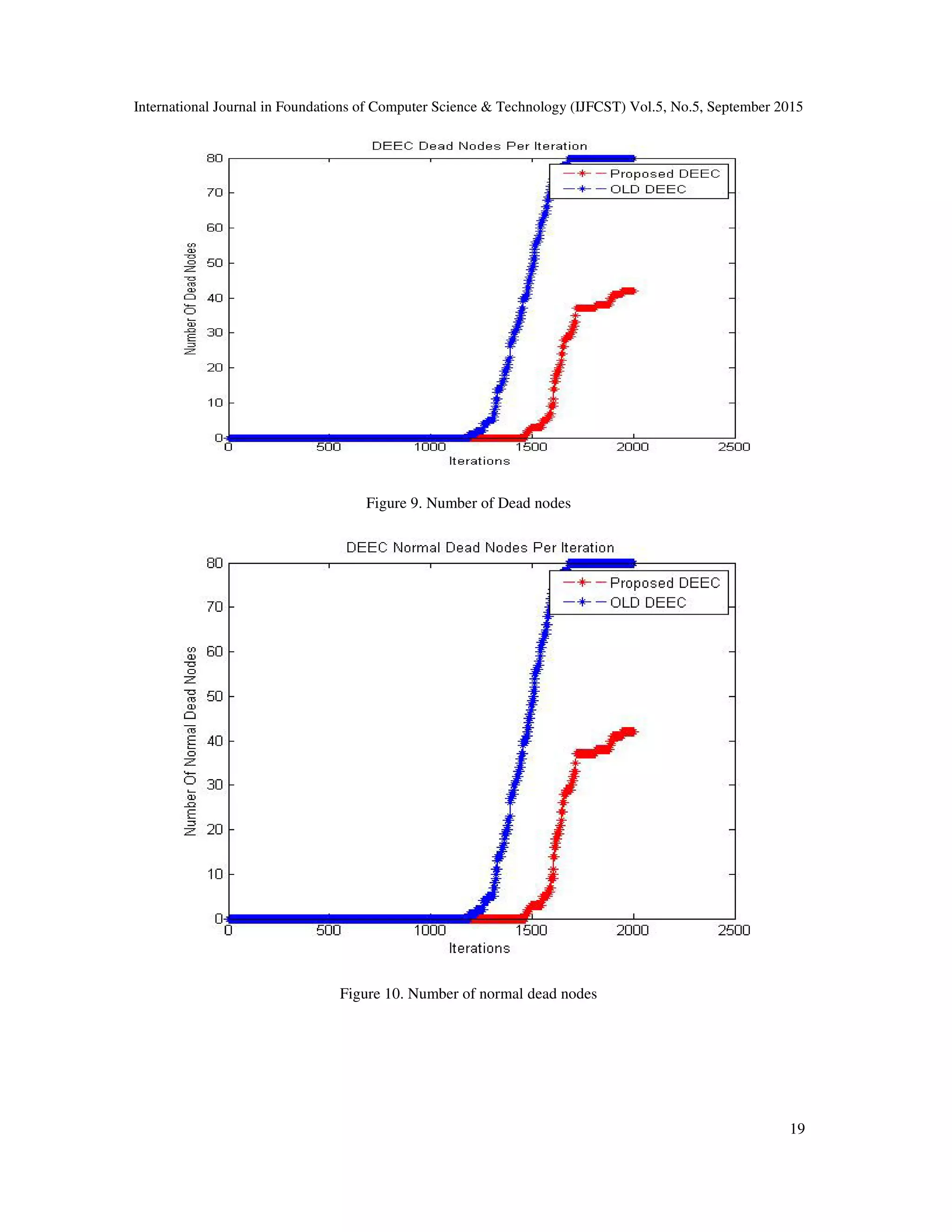
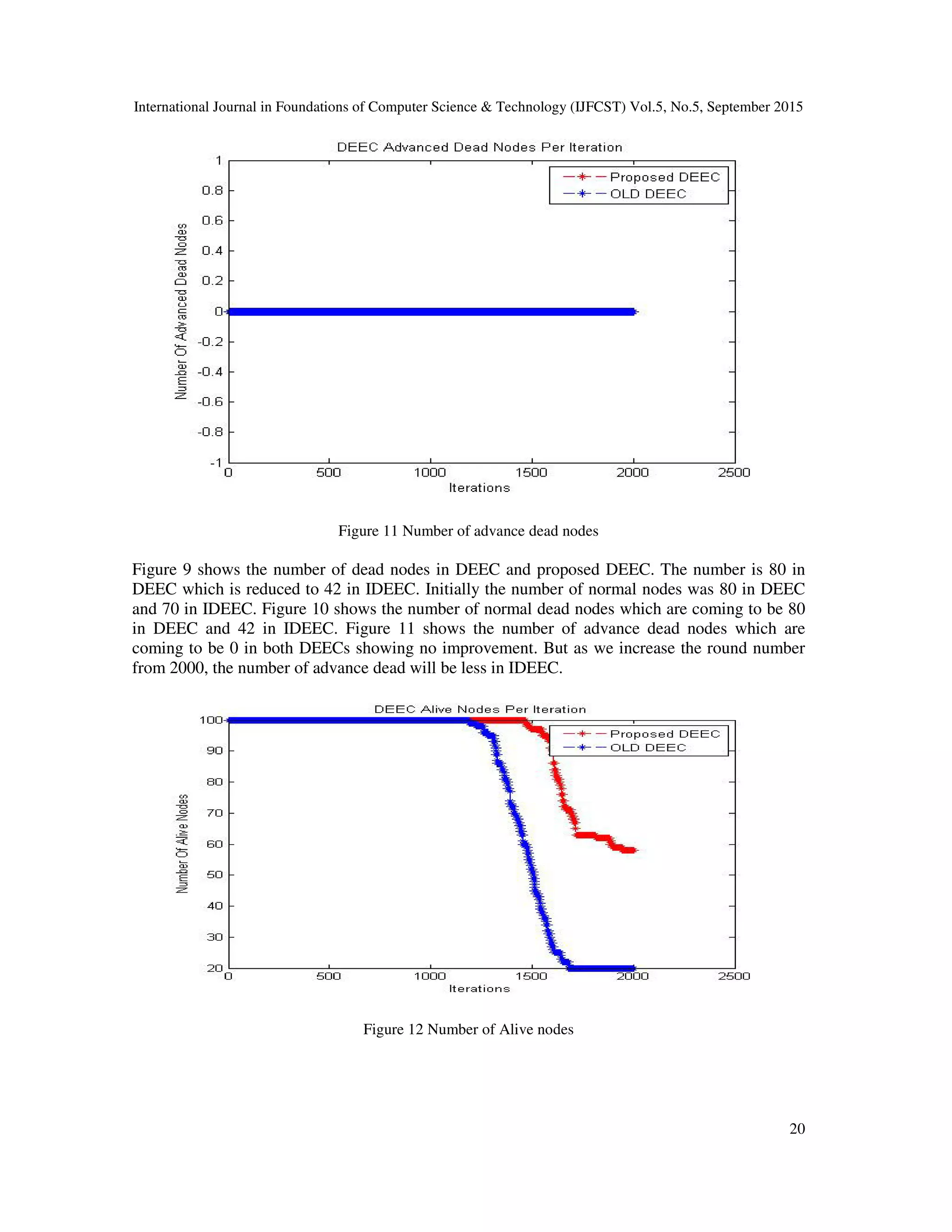
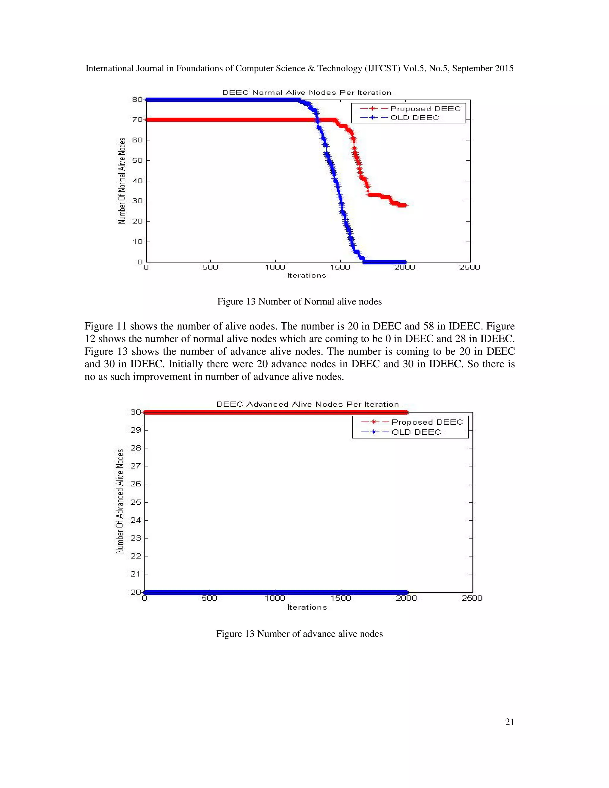
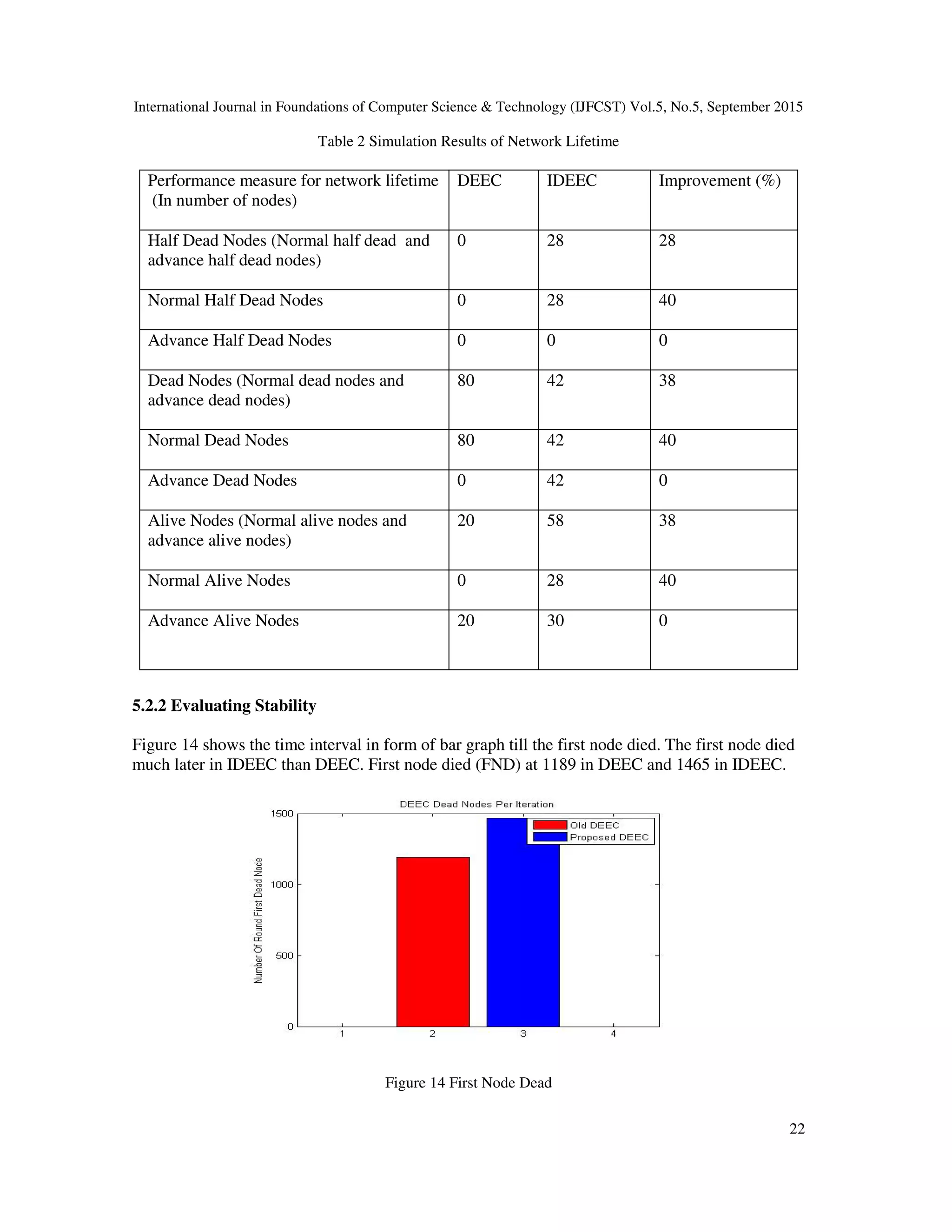
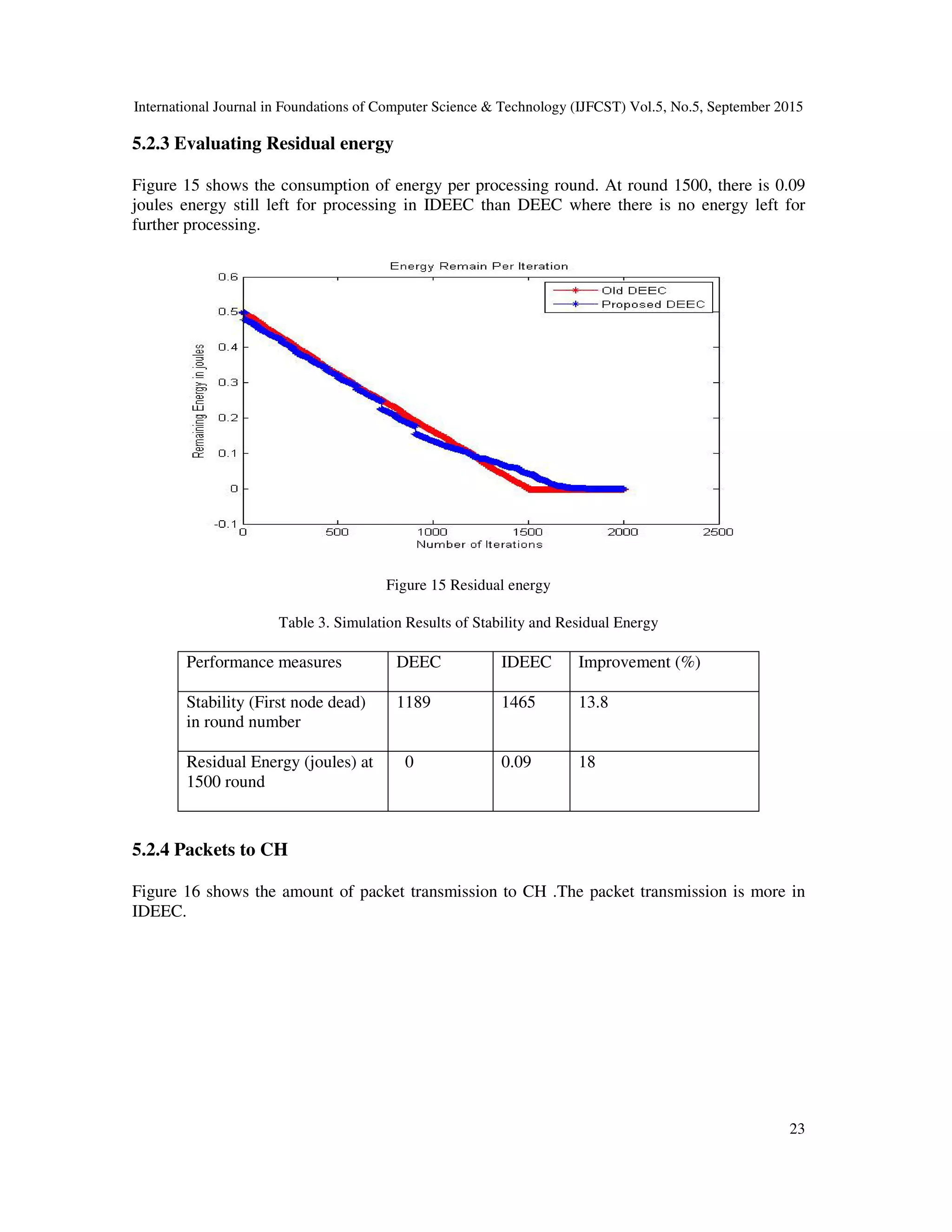
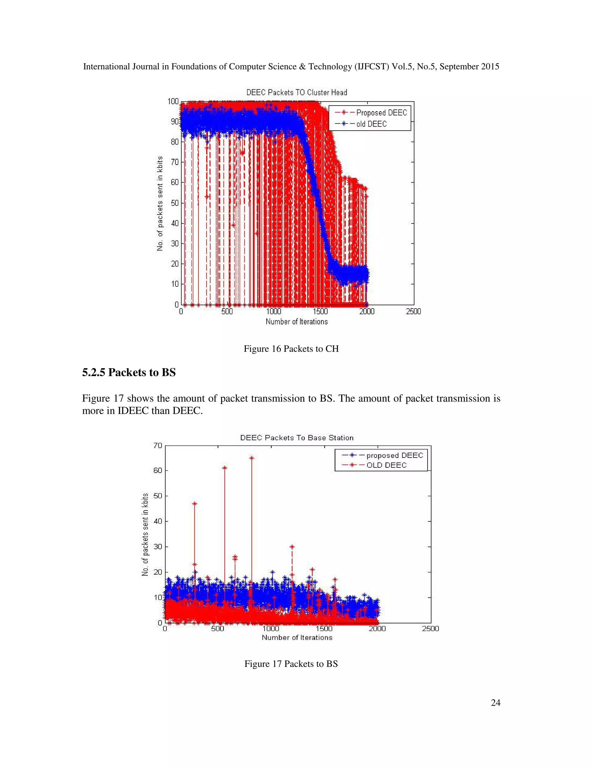
This document presents a multi-hop distributed energy-efficient hierarchical clustering scheme for heterogeneous wireless sensor networks (WSNs), focusing on the development of an enhanced multi-hop DEEC routing protocol. The proposed protocol aims to extend network lifetime by reducing energy consumption during data transmission between sensor nodes and a base station, while utilizing rechargeable intermediate nodes to optimize communication efficiency. Simulation results demonstrate improvements in terms of first dead node occurrence, energy consumption, and data packet transmission compared to existing protocols.