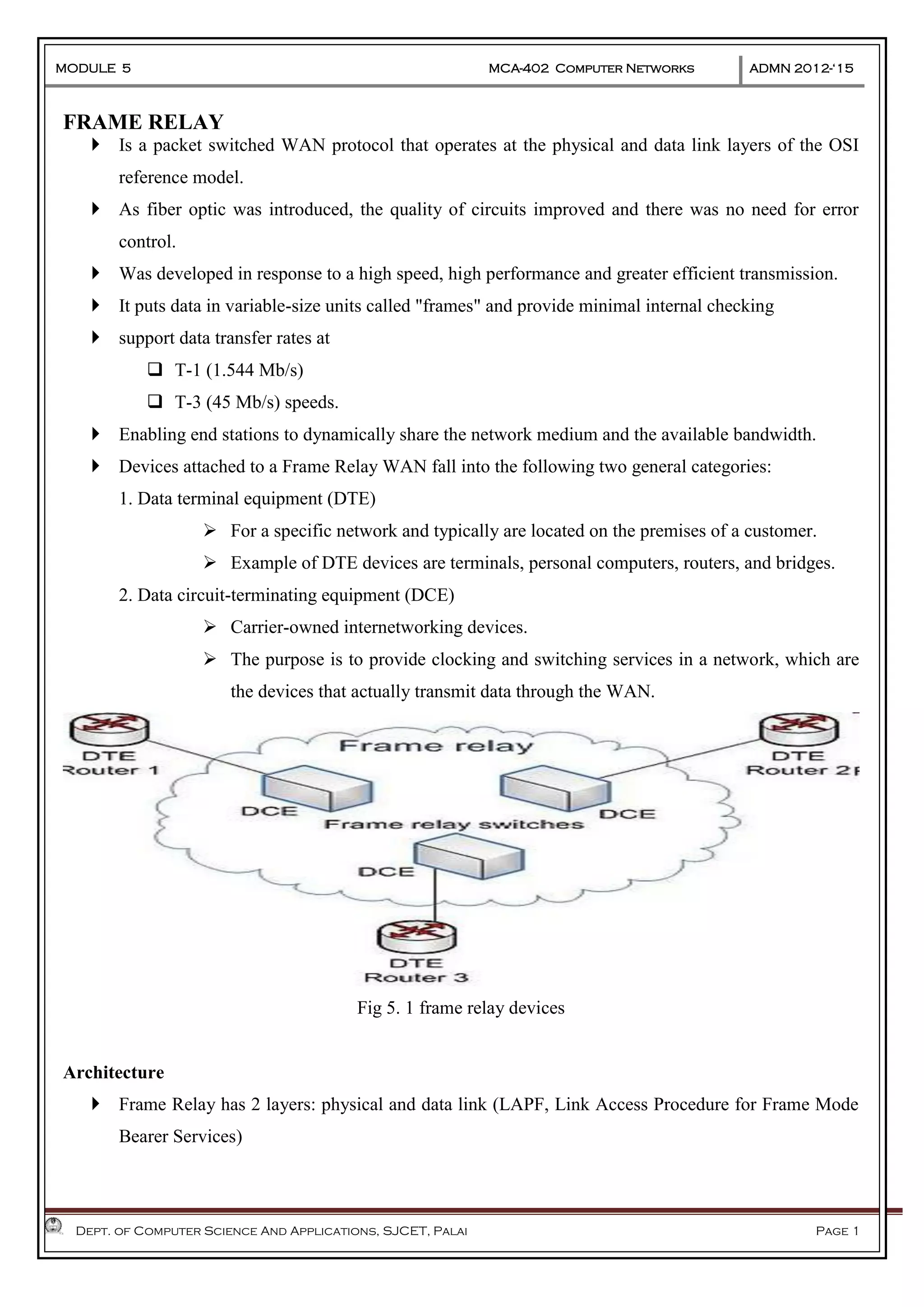
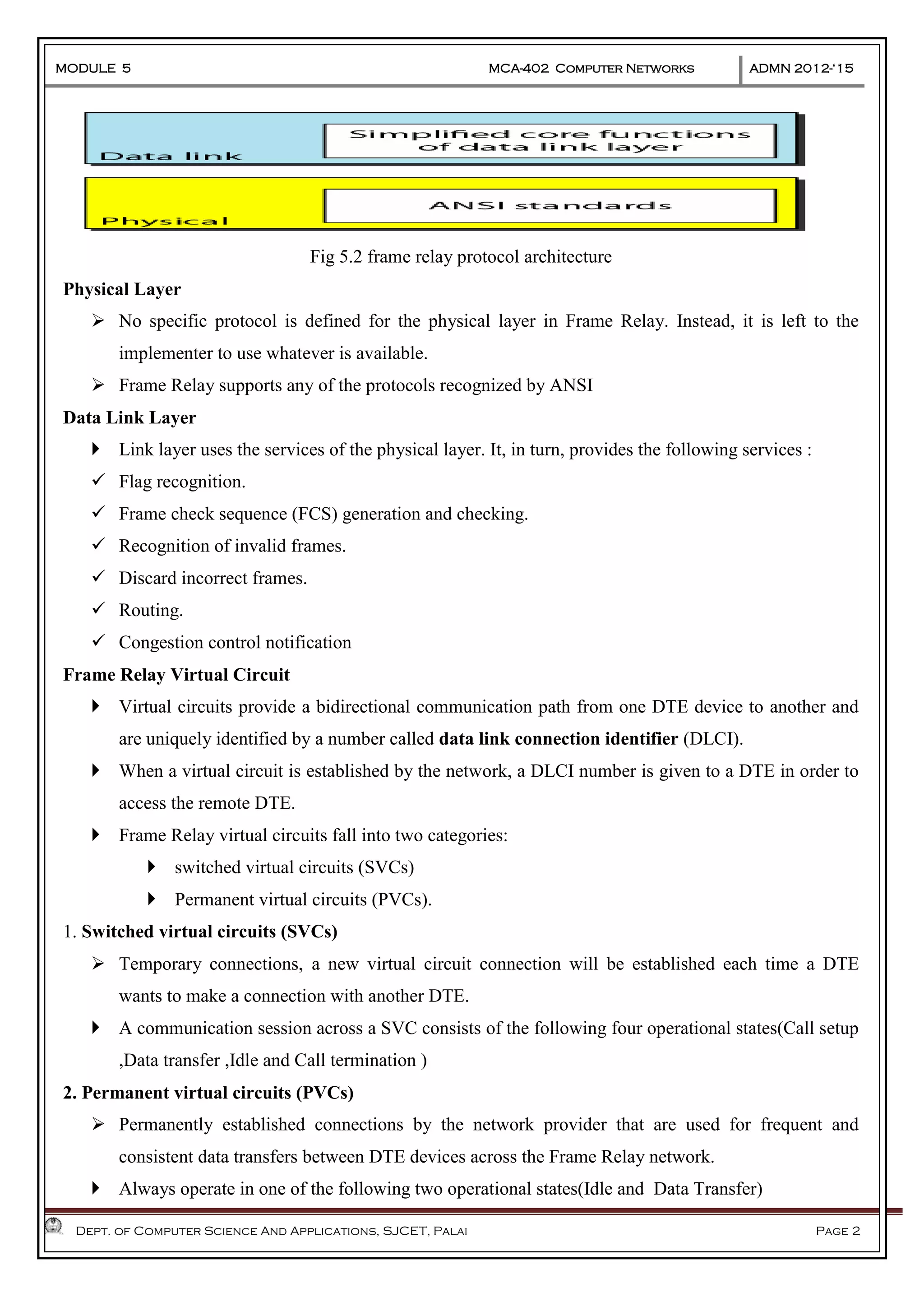
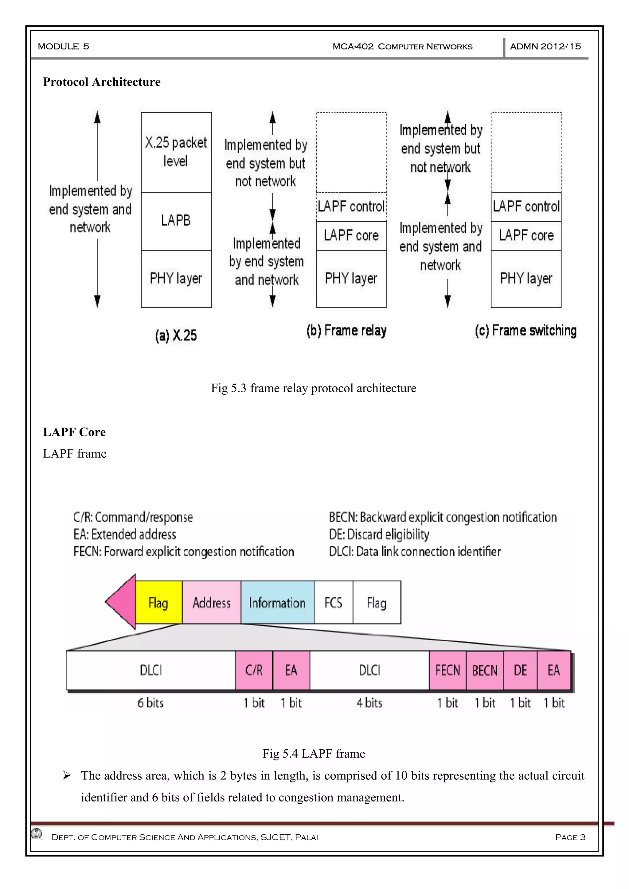
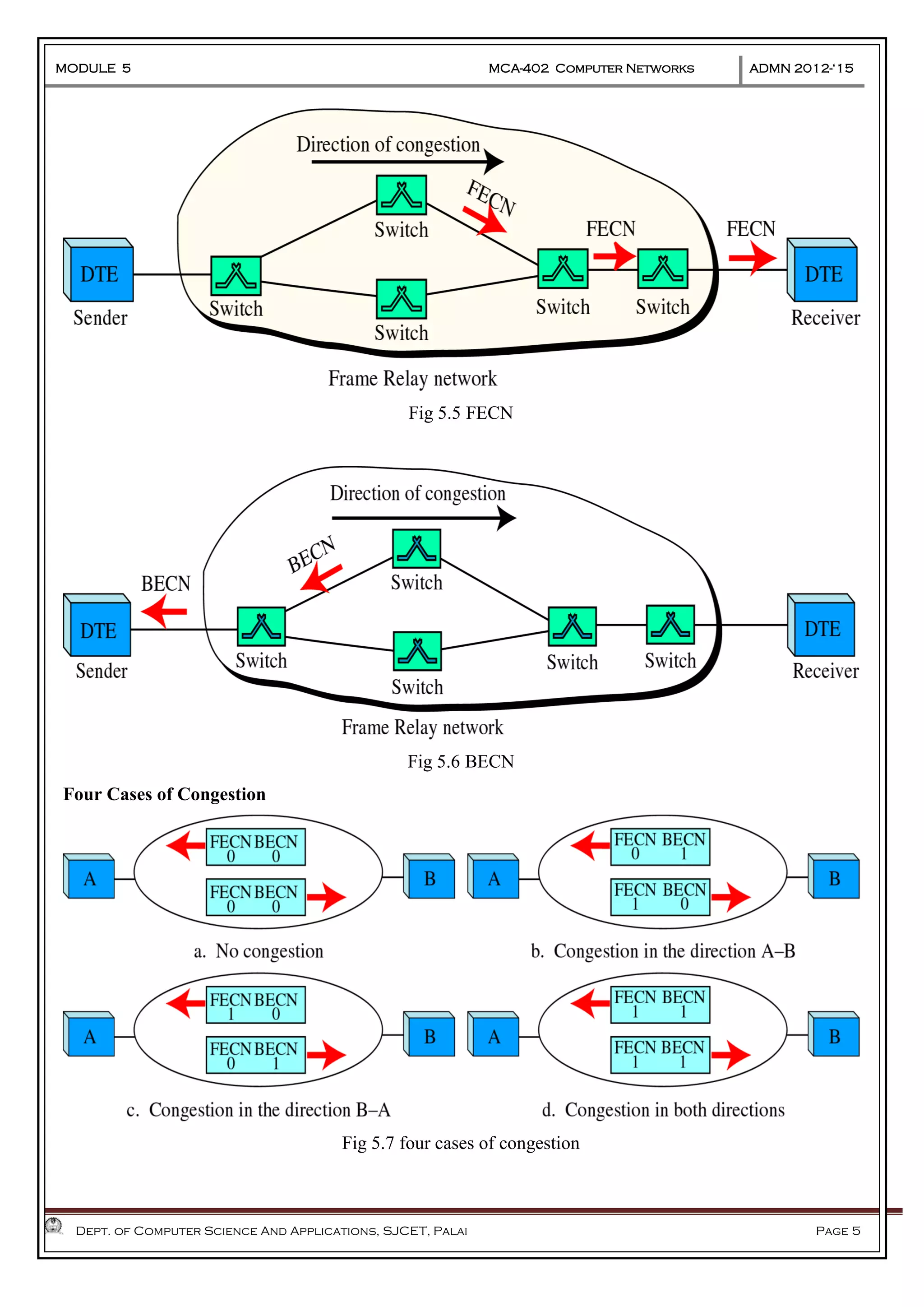
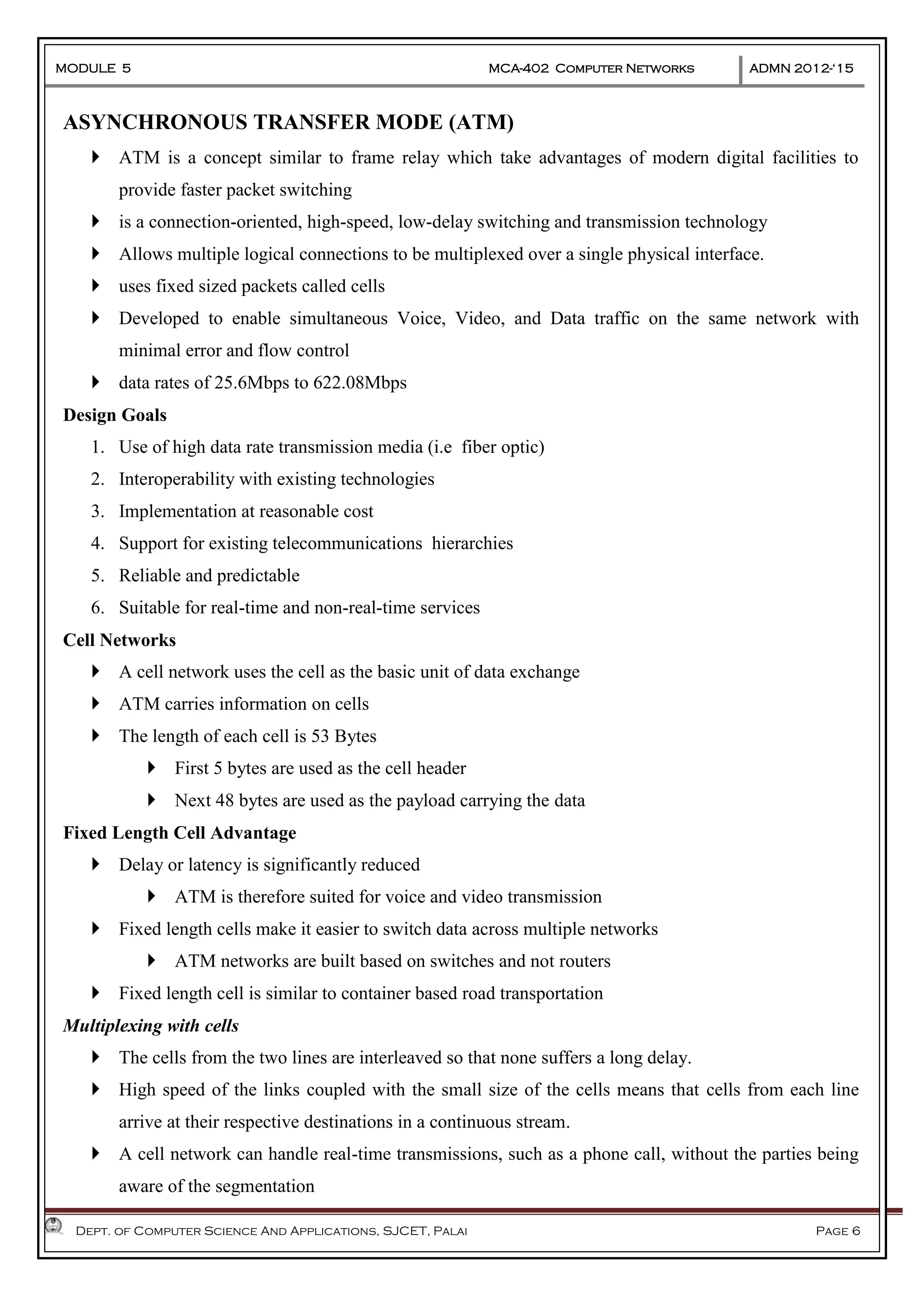
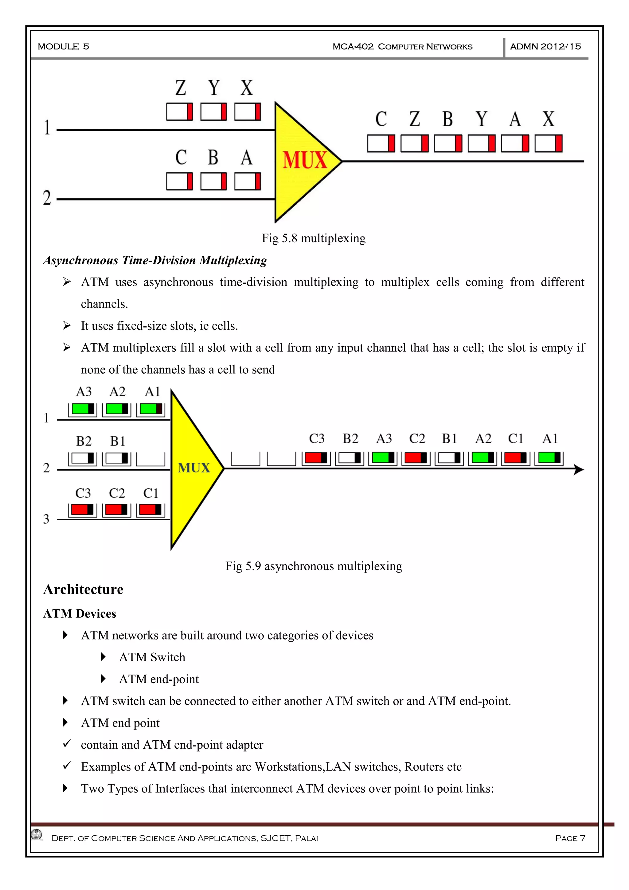
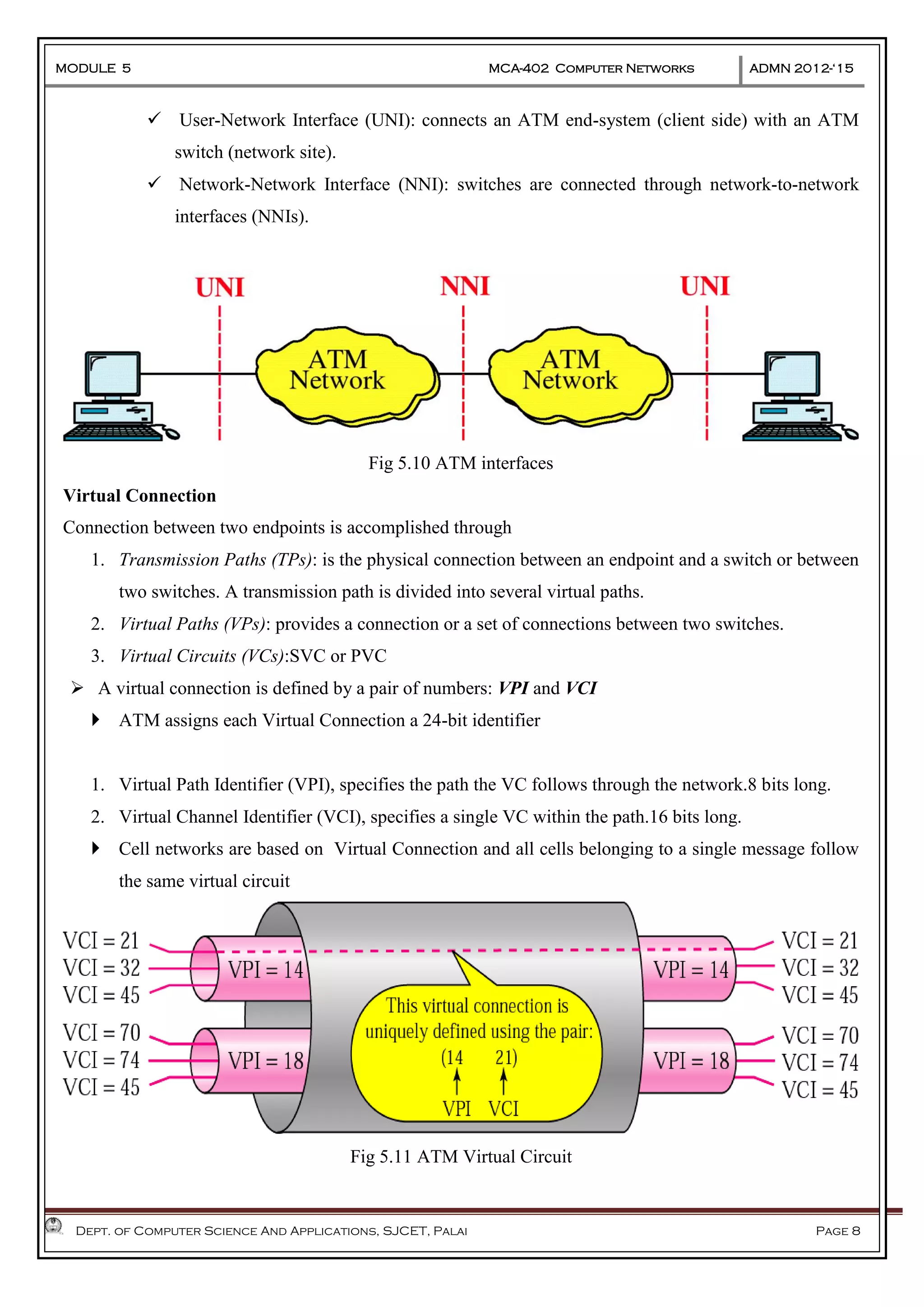
MODULE 5 MCA-402 Computer Networks ADMN 2012-‘15 Dept. of Computer Science And Applications, SJCET, Palai Page 1 FRAME RELAY  Is a packet switched WAN protocol that operates at the physical and data link layers of the OSI reference model.  As fiber optic was introduced, the quality of circuits improved and there was no need for error control.  Was developed in response to a high speed, high performance and greater efficient transmission.  It puts data in variable-size units called "frames" and provide minimal internal checking  support data transfer rates at  T-1 (1.544 Mb/s)  T-3 (45 Mb/s) speeds.  Enabling end stations to dynamically share the network medium and the available bandwidth.  Devices attached to a Frame Relay WAN fall into the following two general categories: 1. Data terminal equipment (DTE)  For a specific network and typically are located on the premises of a customer.  Example of DTE devices are terminals, personal computers, routers, and bridges. 2. Data circuit-terminating equipment (DCE)  Carrier-owned internetworking devices.  The purpose is to provide clocking and switching services in a network, which are the devices that actually transmit data through the WAN. Fig 5. 1 frame relay devices Architecture  Frame Relay has 2 layers: physical and data link (LAPF, Link Access Procedure for Frame Mode Bearer Services)
MODULE 5 MCA-402 Computer Networks ADMN 2012-‘15 Dept. of Computer Science And Applications, SJCET, Palai Page 2 Fig 5.2 frame relay protocol architecture Physical Layer  No specific protocol is defined for the physical layer in Frame Relay. Instead, it is left to the implementer to use whatever is available.  Frame Relay supports any of the protocols recognized by ANSI Data Link Layer  Link layer uses the services of the physical layer. It, in turn, provides the following services :  Flag recognition.  Frame check sequence (FCS) generation and checking.  Recognition of invalid frames.  Discard incorrect frames.  Routing.  Congestion control notification Frame Relay Virtual Circuit  Virtual circuits provide a bidirectional communication path from one DTE device to another and are uniquely identified by a number called data link connection identifier (DLCI).  When a virtual circuit is established by the network, a DLCI number is given to a DTE in order to access the remote DTE.  Frame Relay virtual circuits fall into two categories:  switched virtual circuits (SVCs)  Permanent virtual circuits (PVCs). 1. Switched virtual circuits (SVCs)  Temporary connections, a new virtual circuit connection will be established each time a DTE wants to make a connection with another DTE.  A communication session across a SVC consists of the following four operational states(Call setup ,Data transfer ,Idle and Call termination ) 2. Permanent virtual circuits (PVCs)  Permanently established connections by the network provider that are used for frequent and consistent data transfers between DTE devices across the Frame Relay network.  Always operate in one of the following two operational states(Idle and Data Transfer)
MODULE 5 MCA-402 Computer Networks ADMN 2012-‘15 Dept. of Computer Science And Applications, SJCET, Palai Page 3 Protocol Architecture Fig 5.3 frame relay protocol architecture LAPF Core LAPF frame Fig 5.4 LAPF frame  The address area, which is 2 bytes in length, is comprised of 10 bits representing the actual circuit identifier and 6 bits of fields related to congestion management.
MODULE 5 MCA-402 Computer Networks ADMN 2012-‘15 Dept. of Computer Science And Applications, SJCET, Palai Page 4  DLCI field: 10-bit DLCI field represents the address of the frame and corresponds to a PVC.  Command/response (C/R): Designates whether the frame is a command or response.  Extended address (EA): used for expanding the number of possible addresses.  Forward explicit congestion notification (FECN):can be set by any switch to indicate that traffic is congested. This bit informs the destination that congestion has occurred.  Backward explicit congestion notification (BECN):is set (in frames that travel in the other direction) to indicate a congestion problem in the network.  Discard eligibility (DE): indicates the priority level of the frame. In emergency situations, switches may have to discard frames to relieve bottlenecks and keep the network from collapsing due to overload.  core functions of LAPF are used for frame Relay:  Frame delimiting and transparency  Frame mux and demux using addressing field  Ensure frame is neither too long nor short  Detection of transmission errors  Congestion control functions LAPF-Control  The user terminals (DTEs) implement full LAPF protocol, which is also called LAPF-Control Protocol.  The only difference b/w this protocol and LAPF-core is the inclusion of a control field.  Control protocol provides the functions of flow and error control that are missing from core protocol CONGESTION-CONTROL MECHANISMS  Frame Relay reduces network overhead by implementing simple congestion-notification mechanisms. Frame Relay implements two congestion-notification mechanisms:  Forward-explicit congestion notification (FECN)  Backward-explicit congestion notification (BECN)  FECN and BECN each is controlled by a single bit contained in the Frame Relay frame header. The Frame Relay frame header also contains a Discard Eligibility (DE) bit, which is used to identify less important traffic that can be dropped during periods of congestion.
MODULE 5 MCA-402 Computer Networks ADMN 2012-‘15 Dept. of Computer Science And Applications, SJCET, Palai Page 5 Fig 5.5 FECN Fig 5.6 BECN Four Cases of Congestion Fig 5.7 four cases of congestion
MODULE 5 MCA-402 Computer Networks ADMN 2012-‘15 Dept. of Computer Science And Applications, SJCET, Palai Page 6 ASYNCHRONOUS TRANSFER MODE (ATM)  ATM is a concept similar to frame relay which take advantages of modern digital facilities to provide faster packet switching  is a connection-oriented, high-speed, low-delay switching and transmission technology  Allows multiple logical connections to be multiplexed over a single physical interface.  uses fixed sized packets called cells  Developed to enable simultaneous Voice, Video, and Data traffic on the same network with minimal error and flow control  data rates of 25.6Mbps to 622.08Mbps Design Goals 1. Use of high data rate transmission media (i.e fiber optic) 2. Interoperability with existing technologies 3. Implementation at reasonable cost 4. Support for existing telecommunications hierarchies 5. Reliable and predictable 6. Suitable for real-time and non-real-time services Cell Networks  A cell network uses the cell as the basic unit of data exchange  ATM carries information on cells  The length of each cell is 53 Bytes  First 5 bytes are used as the cell header  Next 48 bytes are used as the payload carrying the data Fixed Length Cell Advantage  Delay or latency is significantly reduced  ATM is therefore suited for voice and video transmission  Fixed length cells make it easier to switch data across multiple networks  ATM networks are built based on switches and not routers  Fixed length cell is similar to container based road transportation Multiplexing with cells  The cells from the two lines are interleaved so that none suffers a long delay.  High speed of the links coupled with the small size of the cells means that cells from each line arrive at their respective destinations in a continuous stream.  A cell network can handle real-time transmissions, such as a phone call, without the parties being aware of the segmentation
MODULE 5 MCA-402 Computer Networks ADMN 2012-‘15 Dept. of Computer Science And Applications, SJCET, Palai Page 7 Fig 5.8 multiplexing Asynchronous Time-Division Multiplexing  ATM uses asynchronous time-division multiplexing to multiplex cells coming from different channels.  It uses fixed-size slots, ie cells.  ATM multiplexers fill a slot with a cell from any input channel that has a cell; the slot is empty if none of the channels has a cell to send Fig 5.9 asynchronous multiplexing Architecture ATM Devices  ATM networks are built around two categories of devices  ATM Switch  ATM end-point  ATM switch can be connected to either another ATM switch or and ATM end-point.  ATM end point  contain and ATM end-point adapter  Examples of ATM end-points are Workstations,LAN switches, Routers etc  Two Types of Interfaces that interconnect ATM devices over point to point links:
MODULE 5 MCA-402 Computer Networks ADMN 2012-‘15 Dept. of Computer Science And Applications, SJCET, Palai Page 8  User-Network Interface (UNI): connects an ATM end-system (client side) with an ATM switch (network site).  Network-Network Interface (NNI): switches are connected through network-to-network interfaces (NNIs). Fig 5.10 ATM interfaces Virtual Connection Connection between two endpoints is accomplished through 1. Transmission Paths (TPs): is the physical connection between an endpoint and a switch or between two switches. A transmission path is divided into several virtual paths. 2. Virtual Paths (VPs): provides a connection or a set of connections between two switches. 3. Virtual Circuits (VCs):SVC or PVC  A virtual connection is defined by a pair of numbers: VPI and VCI  ATM assigns each Virtual Connection a 24-bit identifier 1. Virtual Path Identifier (VPI), specifies the path the VC follows through the network.8 bits long. 2. Virtual Channel Identifier (VCI), specifies a single VC within the path.16 bits long.  Cell networks are based on Virtual Connection and all cells belonging to a single message follow the same virtual circuit Fig 5.11 ATM Virtual Circuit
MODULE 5 MCA-402 Computer Networks ADMN 2012-‘15 Dept. of Computer Science And Applications, SJCET, Palai Page 9 Fig 5. 12 example of virtual path and Virtual Circuit ATM Protocol Layers Fig 5.13 ATM protocol layers Physical Layer  It describes the physical transmission media.  We can use shielded and unshielded twisted pair, coaxial cable, and fiber-optic cable. ATM Layer  The ATM layer is responsible for establishing connections and passing cells through the ATM network.  It provides routing, traffic management, switching, and multiplexing. ATM cell Fig 5.14 ATM cell
MODULE 5 MCA-402 Computer Networks ADMN 2012-‘15 Dept. of Computer Science And Applications, SJCET, Palai Page 10 Fig 5.15 a ATM Cell Header—UNI Format Fig 5.15 b ATM Cell Header—NNI Format  General Flaw Control (GFC): Provides local functions, such as flow control from end point equipment to the ATM switch.  Payload Type (PT): Indicates whether the cell contains user data or control data.  Cell Loss Priority (CLP): Indicates whether the cell should be removed if it encounters errors as it moves through the network.  Header Error Control (HEC): Contains Cyclic Redundancy Check (CRC) on the cell header.  Virtual Path Identifier (VPI): Identifies semi-permanent connections between ATM end points.  Virtual Channel Identifier (VCI): Have only local significance on the link between ATM nodes. ATM Adaptation Layer (AAL)  It converts the submitted information into streams of 48-octet segments and transports these in the payload field of multiple ATM cells.  Similarly, on receipt of the stream of cells it converts the 48-octet information field into required form for delivery to the particular higher protocol layer.  AAL exists only in end systems, not in switches.  AAL Services  Handle transmission errors  Segmentation/reassembly (SAR)  Handle lost and misinserted cell conditions  Flow control and timing control  AAL is classified into four(The classification was made with respect to the ,following parameters:  Timing relationship between sender and receiver  Related
MODULE 5 MCA-402 Computer Networks ADMN 2012-‘15 Dept. of Computer Science And Applications, SJCET, Palai Page 11  Not related  Bit rate  Constant bit rate  Variable bit rate  Connection mode  Connection-oriented  Connectionless  AAL is divided into two sub layers:  Convergence Sub layer: manages the flow of data to and from SAR sub layer.  Segmentation and reassembly sub layer:Packages data from CS into cells and unpacks at other end Fig 5.16 AAL classes AAL 1 (Constant Bit Rate)  The CS layer divides the bit stream into 47-byte segments and passes them to the SAR sub layer below  The SAR sub layer adds 1 byte of header and passes the 48-byte segment to the ATM layer.  The 1 byte header is divided into two 4-bit fields  Sequence number (SN)  Sequence number protection (SNP)
MODULE 5 MCA-402 Computer Networks ADMN 2012-‘15 Dept. of Computer Science And Applications, SJCET, Palai Page 12 Fig 5.17 AAL1 Operation AAL2  AAL2 was intended to support a variable-data-rate bit stream.  It is used for low-bit-rate traffic and short-frame traffic such as audio (compressed or uncompressed), video, or fax  Allows the multiplexing of short frames into one cell.  It widely used in wireless applications Fig 5.18 AAL2 operation AAL 3/4  AAL3 was intended to support connection-oriented data services and AAL4 to support connectionless services  Later they have been combined into a single format called AAL3/4  the convergence sub layer (CS) creates a protocol data unit (PDU) by adding a beginning header to the frame ,a length field as a trailer and a variable-length pad
MODULE 5 MCA-402 Computer Networks ADMN 2012-‘15 Dept. of Computer Science And Applications, SJCET, Palai Page 13  the segmentation and reassembly (SAR) sub layer fragments the PDU and append a header to it .  Then, the SAR sub layer appends a CRC-10 trailer to each PDU fragment for error control  The completed SAR PDU becomes the Payload field of an ATM cell Fig 5.19 AAL3/4 operation AAL 5  Is the primary AAL for data and supports both connection-oriented and connectionless data.  also known as the Simple and Efficient Adaptation Layer (SEAL)  The SAR sub layer simply accepts the CS-PDU and segments it into 48-octet SAR-PDUs without adding any additional fields.  The CS sublayer appends a variable-length pad and an 8-byte trailer to a frame. The trailer includes the length of the frame and a 32-bit cyclic redundancy check (CRC)  The SAR sub layer segments the CS-PDU into 48-byte blocks.  the ATM layer places each block into the Payload field of an ATM cell Fig 5.20 AAL 5
MODULE 5 MCA-402 Computer Networks ADMN 2012-‘15 Dept. of Computer Science And Applications, SJCET, Palai Page 14 TRANSPORT LAYER Introduction  The transport layer is concerned with the provision of host-to-host user connections for the reliable and cost effective transfer of user data  It Isolates upper layers from the network layer  The transport layer is responsible for process-to-process delivery of a packet.  At the transport layer, we need a transport layer address, called a port number, to choose among multiple processes running on the destination host. Transport Services  Provide logical communication between application processes running on different hosts.  There are two types of transport service. The connection-oriented transport service and connection- less transport service.  transport protocols are used for providing transport services .transport protocols run in end systems  sender side: breaks messages into segments, passes to network layer  receiver side: reassembles segments into messages, passes to higher layer  more than one transport protocol available to apps  Internet: TCP and UDP Elements of Transport Protocols 1. Addressing 2. Connection Establishment 3. Connection Release 4. Flow Control and Buffering 5. Multiplexing 6. Crash Recovery 1. Addressing  When an application process wishes to set up a connection to a remote application process, it must specify which one to connect to  The method normally used is to define transport addresses is by using connection requests  The network layer address identifies a host. The transport layer address identifies a user process – a service – running on a host  In the Internet, these endpoints are called ports or TSAP (Transport Services Access Points).  The endpoints in the network layer (i.e., network layer addresses) are called NSAPs (Network Service Access Points).
MODULE 5 MCA-402 Computer Networks ADMN 2012-‘15 Dept. of Computer Science And Applications, SJCET, Palai Page 15 Fig 5.21 TSAPs, NSAPs, and transport connections Fig 5.22 IP addresses versus port numbers 2. Connection Establishment  Just send REQUEST, wait for ACCEPTED.  The problem occurs when the network can lose and duplicate packets.  Main problem is delayed duplicates
MODULE 5 MCA-402 Computer Networks ADMN 2012-‘15 Dept. of Computer Science And Applications, SJCET, Palai Page 16 Fig 5.23 connection establishment strategy  Solutions for delayed duplicates 1. Using throw-away transport addresses  In this approach, each time a new transport address is needed,  When a connection is released, the address is discarded and never used again. 2. Give each connection a connection identifier  Each connection is associated with a connection identifier. Whenever a connection request comes, transport entity update a table with connection.  After each connection is released, each transport entity could update a table listing obsolete connections.  Whenever a connection request comes in, it could be checked against the table, to see if it belonged to a previously-released connection. 3. Setting Packet lifetime  Packet lifetime can be restricted to a known maximum using one of the following techniques:  Restricted subnet design(Any method that prevents packets from looping)  Putting a hop counter in each packet (hop counter incremented every time the packet is forwarded).  Time stamping each packet (Each packet caries the time it was created, with routers agreeing to discard any packets older than a given time Three-way handshake protocol  Used for connection establishment  Each packet is responded to in sequence  Duplicates must be rejected  Three protocol scenarios for three way hand shake a) Normal operation b) Old CONNECTION REQUEST appearing out of nowhere.
MODULE 5 MCA-402 Computer Networks ADMN 2012-‘15 Dept. of Computer Science And Applications, SJCET, Palai Page 17 c) Duplicate CONNECTION REQUEST and duplicate ACK. Fig 5.24 three way hand shake operation (a) Normal operation. (b) Old duplicate CONNECTION REQUEST appearing out of nowhere. (c) Duplicate CONNECTION REQUEST and duplicate ACK. 3. Connection RELEASE  There are two styles of terminating a connection:  asymmetric release  symmetric release Asymmetric release  only 1 peer closes the connection.is abrupt and may cause data loss CR: Connection Request DR: Disconnect Request Fig 5.25 Connection release Asymmetric release The two-army problem
MODULE 5 MCA-402 Computer Networks ADMN 2012-‘15 Dept. of Computer Science And Applications, SJCET, Palai Page 18 Fig 5. 26 two army problem  The blue army has 4 troops (2 on either side of valley) while the white army has 3 troops. If both blue armies charge at the same time they can vanquish the white army. If only one of the blue armies charges it will succumb (3 white troops against 2 blue troops). This means: the blue armies have to synchronize their attack. But in order to synchronize they need to send a messenger through the valley; of course the messenger can get caught by the white army (‘lost packet’). Approach #1: The blue army #1 sends a messenger to tell blue army #2 to attack @ 1400.  Problem: The blue army #1 does not know if the messenger managed to convey message or if he was caught. Thus blue army #1 will not attack. Approach #2: The blue army #2 sends back a messenger to acknowledge to blue army #1 that it got the message.  Problem: The blue army #2 does not know if acknowledge-messenger reached blue army #1. Thus blue army #2 will not attack.  This play can be continued. Symmetric release  Each direction is released independently of the other one.  Four protocol scenarios for releasing a connection:
MODULE 5 MCA-402 Computer Networks ADMN 2012-‘15 Dept. of Computer Science And Applications, SJCET, Palai Page 19 Fig 5.27 four scenarios for symmetric release (a) Normal case of a three-way handshake. (b) Final ACK lost (c) Response lost. (d)Response lost and subsequent DRs lost. 4. Flow control and Buffering  The sender process may send at much higher speed than the receiver process can handle the data thus causing overflow (= packet loss).  Transport layer segments the data stream Fig 5.28 flow control and buffering strategy
MODULE 5 MCA-402 Computer Networks ADMN 2012-‘15 Dept. of Computer Science And Applications, SJCET, Palai Page 20  If most Segments are nearly the same size, it is natural to organize the buffers as a pool of identically-sized buffers, with one Segment per buffer  If there is wide variation in Segment size, a pool of fixed-sized buffers presents problems. Fig 5.29 types of buffering (a) Chained fixed-size buffers. (b) Chained variable-sized buffers. (c) One large circular buffer per connection.  If the buffer size is chosen equal to the largest possible Segment, space will be wasted whenever a short Segment arrives.  If the buffer size is chosen less than the maximum Segment size, multiple buffers will be needed for long Segments, with the attendant complexity.  Another approach to the buffer size problem is to use variable-sized buffers.  The advantage here is better memory utilization, at the price of more complicated buffer management.  A third possibility is to dedicate a single large circular buffer per connection  This system is simple and elegant and does not depend on segment sizes, but makes good use of memory only when the connections are heavily loaded. 4. Multiplexing & De-multiplexing  In the transport layer the need for multiplexing can arise in a number of ways.  There are two types of multiplexing i. Upward ii. Downward
MODULE 5 MCA-402 Computer Networks ADMN 2012-‘15 Dept. of Computer Science And Applications, SJCET, Palai Page 21 Fig 5.30 multiplexing and multiplexing i. Upward multiplexing  Traffic from a “data stream” is distributed over several transport connections (TSAPs).  For Eg, if only one network address is available on a host, all transport connections on that machine have to use it. Fig 5.31 upward multiplexing ii. Downward Multiplexing  Many “data streams” share the same transport connection using multiple NSAPs, possibly over multiple network interfaces (load balancing). Fig 5.32 downward multiplexing
MODULE 5 MCA-402 Computer Networks ADMN 2012-‘15 Dept. of Computer Science And Applications, SJCET, Palai Page 22 6. Crash Recovery  A crash of one host (server) during the transmission leads to a connection loss which results in data loss. Solution for this, the client retransmits only unacknowledged packets.  Does not work in all cases Fig 5.33 normal crash recovery mechanism  A crash at layer N can only be handled at layer N+1 (a system crash is a crash at every layer).  Thus: It is left to the application layer to handle crashes of the remote host (client or server).  Generally applications detect that the remote host has died and then simply restart the connection and retransmit everything.  Each client can be in one of two states i. S1: 1 unacknowledged packet outstanding ii. S0:No unacknowledged packet outstanding  The server can be programmed in one of two ways i. First ACK, then write ii. First write, then ACK  The client can be programmed in one of four ways i. always retransmit the last segment, ii. never retransmit the last segment, iii. retransmit only in state S0, iv. Retransmit only in state S1.
MODULE 5 MCA-402 Computer Networks ADMN 2012-‘15 Dept. of Computer Science And Applications, SJCET, Palai Page 23  Three events are possible at the server i. sending an ack (A), ii. writing to the output process (W), iii. crashing (C) Fig 5.34 crash recovery states A SIMPLE TRANSPORT PROTOCOL  Transport Service Primitives allows transport users (e.g., application programs) to access transport service. Five primitives: CONNECT, LISTEN, DISCONNECT, SEND and RECEIVE. Fig 5.35 connection primitives
MODULE 5 MCA-402 Computer Networks ADMN 2012-‘15 Dept. of Computer Science And Applications, SJCET, Palai Page 24  The parameters for the service primitives and library procedures are as follows: connum = LISTEN(local) connum = CONNECT(local, remote) status = SEND(connum, buffer, bytes) status = RECEIVE(connum, buffer, bytes) status = DISCONNECT(connum)  The LISTEN primitive announces the caller's willingness to accept connection requests directed at the indicated TSAP.  The CONNECT primitive takes two parameters, a local TSAP (i.e., transport address), local, and a remote TSAP, remote, and tries to establish a transport connection between the two.If it succeeds, it returns in connum a nonnegative otherwise a negative number  The SEND primitive transmits the contents of the buffer as a message on the indicated transport connection, in several units if needed. Possible errors, returned in status, are no connection, illegal buffer address.  The RECEIVE primitive indicates the caller's desire to accept data. The size of the incoming message is placed in bytes. If the remote process has released the connection or the buffer address is illegal, status is set to an error code indicating the nature of the problem  The DISCONNECT primitive terminates a transport connection. The parameter connum tells which one.  Possible errors are connum belongs to another process or connum is not a valid connection identifier.  The transport layer makes use of the network service primitives to send and receive TPDUs.  The hardware and/or software within the transport layer that does the work is called the transport entity. Fig 5.36 network packets in transport layer
MODULE 5 MCA-402 Computer Networks ADMN 2012-‘15 Dept. of Computer Science And Applications, SJCET, Palai Page 25  Transport entity: states of a connection Fig 5.37 states of transport entity

Module 4 netwok layer,routing ,vlan,x.25doc

  • 1.
    MODULE 5 MCA-402Computer Networks ADMN 2012-‘15 Dept. of Computer Science And Applications, SJCET, Palai Page 1 FRAME RELAY  Is a packet switched WAN protocol that operates at the physical and data link layers of the OSI reference model.  As fiber optic was introduced, the quality of circuits improved and there was no need for error control.  Was developed in response to a high speed, high performance and greater efficient transmission.  It puts data in variable-size units called "frames" and provide minimal internal checking  support data transfer rates at  T-1 (1.544 Mb/s)  T-3 (45 Mb/s) speeds.  Enabling end stations to dynamically share the network medium and the available bandwidth.  Devices attached to a Frame Relay WAN fall into the following two general categories: 1. Data terminal equipment (DTE)  For a specific network and typically are located on the premises of a customer.  Example of DTE devices are terminals, personal computers, routers, and bridges. 2. Data circuit-terminating equipment (DCE)  Carrier-owned internetworking devices.  The purpose is to provide clocking and switching services in a network, which are the devices that actually transmit data through the WAN. Fig 5. 1 frame relay devices Architecture  Frame Relay has 2 layers: physical and data link (LAPF, Link Access Procedure for Frame Mode Bearer Services)
  • 2.
    MODULE 5 MCA-402Computer Networks ADMN 2012-‘15 Dept. of Computer Science And Applications, SJCET, Palai Page 2 Fig 5.2 frame relay protocol architecture Physical Layer  No specific protocol is defined for the physical layer in Frame Relay. Instead, it is left to the implementer to use whatever is available.  Frame Relay supports any of the protocols recognized by ANSI Data Link Layer  Link layer uses the services of the physical layer. It, in turn, provides the following services :  Flag recognition.  Frame check sequence (FCS) generation and checking.  Recognition of invalid frames.  Discard incorrect frames.  Routing.  Congestion control notification Frame Relay Virtual Circuit  Virtual circuits provide a bidirectional communication path from one DTE device to another and are uniquely identified by a number called data link connection identifier (DLCI).  When a virtual circuit is established by the network, a DLCI number is given to a DTE in order to access the remote DTE.  Frame Relay virtual circuits fall into two categories:  switched virtual circuits (SVCs)  Permanent virtual circuits (PVCs). 1. Switched virtual circuits (SVCs)  Temporary connections, a new virtual circuit connection will be established each time a DTE wants to make a connection with another DTE.  A communication session across a SVC consists of the following four operational states(Call setup ,Data transfer ,Idle and Call termination ) 2. Permanent virtual circuits (PVCs)  Permanently established connections by the network provider that are used for frequent and consistent data transfers between DTE devices across the Frame Relay network.  Always operate in one of the following two operational states(Idle and Data Transfer)
  • 3.
    MODULE 5 MCA-402Computer Networks ADMN 2012-‘15 Dept. of Computer Science And Applications, SJCET, Palai Page 3 Protocol Architecture Fig 5.3 frame relay protocol architecture LAPF Core LAPF frame Fig 5.4 LAPF frame  The address area, which is 2 bytes in length, is comprised of 10 bits representing the actual circuit identifier and 6 bits of fields related to congestion management.
  • 4.
    MODULE 5 MCA-402Computer Networks ADMN 2012-‘15 Dept. of Computer Science And Applications, SJCET, Palai Page 4  DLCI field: 10-bit DLCI field represents the address of the frame and corresponds to a PVC.  Command/response (C/R): Designates whether the frame is a command or response.  Extended address (EA): used for expanding the number of possible addresses.  Forward explicit congestion notification (FECN):can be set by any switch to indicate that traffic is congested. This bit informs the destination that congestion has occurred.  Backward explicit congestion notification (BECN):is set (in frames that travel in the other direction) to indicate a congestion problem in the network.  Discard eligibility (DE): indicates the priority level of the frame. In emergency situations, switches may have to discard frames to relieve bottlenecks and keep the network from collapsing due to overload.  core functions of LAPF are used for frame Relay:  Frame delimiting and transparency  Frame mux and demux using addressing field  Ensure frame is neither too long nor short  Detection of transmission errors  Congestion control functions LAPF-Control  The user terminals (DTEs) implement full LAPF protocol, which is also called LAPF-Control Protocol.  The only difference b/w this protocol and LAPF-core is the inclusion of a control field.  Control protocol provides the functions of flow and error control that are missing from core protocol CONGESTION-CONTROL MECHANISMS  Frame Relay reduces network overhead by implementing simple congestion-notification mechanisms. Frame Relay implements two congestion-notification mechanisms:  Forward-explicit congestion notification (FECN)  Backward-explicit congestion notification (BECN)  FECN and BECN each is controlled by a single bit contained in the Frame Relay frame header. The Frame Relay frame header also contains a Discard Eligibility (DE) bit, which is used to identify less important traffic that can be dropped during periods of congestion.
  • 5.
    MODULE 5 MCA-402Computer Networks ADMN 2012-‘15 Dept. of Computer Science And Applications, SJCET, Palai Page 5 Fig 5.5 FECN Fig 5.6 BECN Four Cases of Congestion Fig 5.7 four cases of congestion
  • 6.
    MODULE 5 MCA-402Computer Networks ADMN 2012-‘15 Dept. of Computer Science And Applications, SJCET, Palai Page 6 ASYNCHRONOUS TRANSFER MODE (ATM)  ATM is a concept similar to frame relay which take advantages of modern digital facilities to provide faster packet switching  is a connection-oriented, high-speed, low-delay switching and transmission technology  Allows multiple logical connections to be multiplexed over a single physical interface.  uses fixed sized packets called cells  Developed to enable simultaneous Voice, Video, and Data traffic on the same network with minimal error and flow control  data rates of 25.6Mbps to 622.08Mbps Design Goals 1. Use of high data rate transmission media (i.e fiber optic) 2. Interoperability with existing technologies 3. Implementation at reasonable cost 4. Support for existing telecommunications hierarchies 5. Reliable and predictable 6. Suitable for real-time and non-real-time services Cell Networks  A cell network uses the cell as the basic unit of data exchange  ATM carries information on cells  The length of each cell is 53 Bytes  First 5 bytes are used as the cell header  Next 48 bytes are used as the payload carrying the data Fixed Length Cell Advantage  Delay or latency is significantly reduced  ATM is therefore suited for voice and video transmission  Fixed length cells make it easier to switch data across multiple networks  ATM networks are built based on switches and not routers  Fixed length cell is similar to container based road transportation Multiplexing with cells  The cells from the two lines are interleaved so that none suffers a long delay.  High speed of the links coupled with the small size of the cells means that cells from each line arrive at their respective destinations in a continuous stream.  A cell network can handle real-time transmissions, such as a phone call, without the parties being aware of the segmentation
  • 7.
    MODULE 5 MCA-402Computer Networks ADMN 2012-‘15 Dept. of Computer Science And Applications, SJCET, Palai Page 7 Fig 5.8 multiplexing Asynchronous Time-Division Multiplexing  ATM uses asynchronous time-division multiplexing to multiplex cells coming from different channels.  It uses fixed-size slots, ie cells.  ATM multiplexers fill a slot with a cell from any input channel that has a cell; the slot is empty if none of the channels has a cell to send Fig 5.9 asynchronous multiplexing Architecture ATM Devices  ATM networks are built around two categories of devices  ATM Switch  ATM end-point  ATM switch can be connected to either another ATM switch or and ATM end-point.  ATM end point  contain and ATM end-point adapter  Examples of ATM end-points are Workstations,LAN switches, Routers etc  Two Types of Interfaces that interconnect ATM devices over point to point links:
  • 8.
    MODULE 5 MCA-402Computer Networks ADMN 2012-‘15 Dept. of Computer Science And Applications, SJCET, Palai Page 8  User-Network Interface (UNI): connects an ATM end-system (client side) with an ATM switch (network site).  Network-Network Interface (NNI): switches are connected through network-to-network interfaces (NNIs). Fig 5.10 ATM interfaces Virtual Connection Connection between two endpoints is accomplished through 1. Transmission Paths (TPs): is the physical connection between an endpoint and a switch or between two switches. A transmission path is divided into several virtual paths. 2. Virtual Paths (VPs): provides a connection or a set of connections between two switches. 3. Virtual Circuits (VCs):SVC or PVC  A virtual connection is defined by a pair of numbers: VPI and VCI  ATM assigns each Virtual Connection a 24-bit identifier 1. Virtual Path Identifier (VPI), specifies the path the VC follows through the network.8 bits long. 2. Virtual Channel Identifier (VCI), specifies a single VC within the path.16 bits long.  Cell networks are based on Virtual Connection and all cells belonging to a single message follow the same virtual circuit Fig 5.11 ATM Virtual Circuit
  • 9.
    MODULE 5 MCA-402Computer Networks ADMN 2012-‘15 Dept. of Computer Science And Applications, SJCET, Palai Page 9 Fig 5. 12 example of virtual path and Virtual Circuit ATM Protocol Layers Fig 5.13 ATM protocol layers Physical Layer  It describes the physical transmission media.  We can use shielded and unshielded twisted pair, coaxial cable, and fiber-optic cable. ATM Layer  The ATM layer is responsible for establishing connections and passing cells through the ATM network.  It provides routing, traffic management, switching, and multiplexing. ATM cell Fig 5.14 ATM cell
  • 10.
    MODULE 5 MCA-402Computer Networks ADMN 2012-‘15 Dept. of Computer Science And Applications, SJCET, Palai Page 10 Fig 5.15 a ATM Cell Header—UNI Format Fig 5.15 b ATM Cell Header—NNI Format  General Flaw Control (GFC): Provides local functions, such as flow control from end point equipment to the ATM switch.  Payload Type (PT): Indicates whether the cell contains user data or control data.  Cell Loss Priority (CLP): Indicates whether the cell should be removed if it encounters errors as it moves through the network.  Header Error Control (HEC): Contains Cyclic Redundancy Check (CRC) on the cell header.  Virtual Path Identifier (VPI): Identifies semi-permanent connections between ATM end points.  Virtual Channel Identifier (VCI): Have only local significance on the link between ATM nodes. ATM Adaptation Layer (AAL)  It converts the submitted information into streams of 48-octet segments and transports these in the payload field of multiple ATM cells.  Similarly, on receipt of the stream of cells it converts the 48-octet information field into required form for delivery to the particular higher protocol layer.  AAL exists only in end systems, not in switches.  AAL Services  Handle transmission errors  Segmentation/reassembly (SAR)  Handle lost and misinserted cell conditions  Flow control and timing control  AAL is classified into four(The classification was made with respect to the ,following parameters:  Timing relationship between sender and receiver  Related
  • 11.
    MODULE 5 MCA-402Computer Networks ADMN 2012-‘15 Dept. of Computer Science And Applications, SJCET, Palai Page 11  Not related  Bit rate  Constant bit rate  Variable bit rate  Connection mode  Connection-oriented  Connectionless  AAL is divided into two sub layers:  Convergence Sub layer: manages the flow of data to and from SAR sub layer.  Segmentation and reassembly sub layer:Packages data from CS into cells and unpacks at other end Fig 5.16 AAL classes AAL 1 (Constant Bit Rate)  The CS layer divides the bit stream into 47-byte segments and passes them to the SAR sub layer below  The SAR sub layer adds 1 byte of header and passes the 48-byte segment to the ATM layer.  The 1 byte header is divided into two 4-bit fields  Sequence number (SN)  Sequence number protection (SNP)
  • 12.
    MODULE 5 MCA-402Computer Networks ADMN 2012-‘15 Dept. of Computer Science And Applications, SJCET, Palai Page 12 Fig 5.17 AAL1 Operation AAL2  AAL2 was intended to support a variable-data-rate bit stream.  It is used for low-bit-rate traffic and short-frame traffic such as audio (compressed or uncompressed), video, or fax  Allows the multiplexing of short frames into one cell.  It widely used in wireless applications Fig 5.18 AAL2 operation AAL 3/4  AAL3 was intended to support connection-oriented data services and AAL4 to support connectionless services  Later they have been combined into a single format called AAL3/4  the convergence sub layer (CS) creates a protocol data unit (PDU) by adding a beginning header to the frame ,a length field as a trailer and a variable-length pad
  • 13.
    MODULE 5 MCA-402Computer Networks ADMN 2012-‘15 Dept. of Computer Science And Applications, SJCET, Palai Page 13  the segmentation and reassembly (SAR) sub layer fragments the PDU and append a header to it .  Then, the SAR sub layer appends a CRC-10 trailer to each PDU fragment for error control  The completed SAR PDU becomes the Payload field of an ATM cell Fig 5.19 AAL3/4 operation AAL 5  Is the primary AAL for data and supports both connection-oriented and connectionless data.  also known as the Simple and Efficient Adaptation Layer (SEAL)  The SAR sub layer simply accepts the CS-PDU and segments it into 48-octet SAR-PDUs without adding any additional fields.  The CS sublayer appends a variable-length pad and an 8-byte trailer to a frame. The trailer includes the length of the frame and a 32-bit cyclic redundancy check (CRC)  The SAR sub layer segments the CS-PDU into 48-byte blocks.  the ATM layer places each block into the Payload field of an ATM cell Fig 5.20 AAL 5
  • 14.
    MODULE 5 MCA-402Computer Networks ADMN 2012-‘15 Dept. of Computer Science And Applications, SJCET, Palai Page 14 TRANSPORT LAYER Introduction  The transport layer is concerned with the provision of host-to-host user connections for the reliable and cost effective transfer of user data  It Isolates upper layers from the network layer  The transport layer is responsible for process-to-process delivery of a packet.  At the transport layer, we need a transport layer address, called a port number, to choose among multiple processes running on the destination host. Transport Services  Provide logical communication between application processes running on different hosts.  There are two types of transport service. The connection-oriented transport service and connection- less transport service.  transport protocols are used for providing transport services .transport protocols run in end systems  sender side: breaks messages into segments, passes to network layer  receiver side: reassembles segments into messages, passes to higher layer  more than one transport protocol available to apps  Internet: TCP and UDP Elements of Transport Protocols 1. Addressing 2. Connection Establishment 3. Connection Release 4. Flow Control and Buffering 5. Multiplexing 6. Crash Recovery 1. Addressing  When an application process wishes to set up a connection to a remote application process, it must specify which one to connect to  The method normally used is to define transport addresses is by using connection requests  The network layer address identifies a host. The transport layer address identifies a user process – a service – running on a host  In the Internet, these endpoints are called ports or TSAP (Transport Services Access Points).  The endpoints in the network layer (i.e., network layer addresses) are called NSAPs (Network Service Access Points).
  • 15.
    MODULE 5 MCA-402Computer Networks ADMN 2012-‘15 Dept. of Computer Science And Applications, SJCET, Palai Page 15 Fig 5.21 TSAPs, NSAPs, and transport connections Fig 5.22 IP addresses versus port numbers 2. Connection Establishment  Just send REQUEST, wait for ACCEPTED.  The problem occurs when the network can lose and duplicate packets.  Main problem is delayed duplicates
  • 16.
    MODULE 5 MCA-402Computer Networks ADMN 2012-‘15 Dept. of Computer Science And Applications, SJCET, Palai Page 16 Fig 5.23 connection establishment strategy  Solutions for delayed duplicates 1. Using throw-away transport addresses  In this approach, each time a new transport address is needed,  When a connection is released, the address is discarded and never used again. 2. Give each connection a connection identifier  Each connection is associated with a connection identifier. Whenever a connection request comes, transport entity update a table with connection.  After each connection is released, each transport entity could update a table listing obsolete connections.  Whenever a connection request comes in, it could be checked against the table, to see if it belonged to a previously-released connection. 3. Setting Packet lifetime  Packet lifetime can be restricted to a known maximum using one of the following techniques:  Restricted subnet design(Any method that prevents packets from looping)  Putting a hop counter in each packet (hop counter incremented every time the packet is forwarded).  Time stamping each packet (Each packet caries the time it was created, with routers agreeing to discard any packets older than a given time Three-way handshake protocol  Used for connection establishment  Each packet is responded to in sequence  Duplicates must be rejected  Three protocol scenarios for three way hand shake a) Normal operation b) Old CONNECTION REQUEST appearing out of nowhere.
  • 17.
    MODULE 5 MCA-402Computer Networks ADMN 2012-‘15 Dept. of Computer Science And Applications, SJCET, Palai Page 17 c) Duplicate CONNECTION REQUEST and duplicate ACK. Fig 5.24 three way hand shake operation (a) Normal operation. (b) Old duplicate CONNECTION REQUEST appearing out of nowhere. (c) Duplicate CONNECTION REQUEST and duplicate ACK. 3. Connection RELEASE  There are two styles of terminating a connection:  asymmetric release  symmetric release Asymmetric release  only 1 peer closes the connection.is abrupt and may cause data loss CR: Connection Request DR: Disconnect Request Fig 5.25 Connection release Asymmetric release The two-army problem
  • 18.
    MODULE 5 MCA-402Computer Networks ADMN 2012-‘15 Dept. of Computer Science And Applications, SJCET, Palai Page 18 Fig 5. 26 two army problem  The blue army has 4 troops (2 on either side of valley) while the white army has 3 troops. If both blue armies charge at the same time they can vanquish the white army. If only one of the blue armies charges it will succumb (3 white troops against 2 blue troops). This means: the blue armies have to synchronize their attack. But in order to synchronize they need to send a messenger through the valley; of course the messenger can get caught by the white army (‘lost packet’). Approach #1: The blue army #1 sends a messenger to tell blue army #2 to attack @ 1400.  Problem: The blue army #1 does not know if the messenger managed to convey message or if he was caught. Thus blue army #1 will not attack. Approach #2: The blue army #2 sends back a messenger to acknowledge to blue army #1 that it got the message.  Problem: The blue army #2 does not know if acknowledge-messenger reached blue army #1. Thus blue army #2 will not attack.  This play can be continued. Symmetric release  Each direction is released independently of the other one.  Four protocol scenarios for releasing a connection:
  • 19.
    MODULE 5 MCA-402Computer Networks ADMN 2012-‘15 Dept. of Computer Science And Applications, SJCET, Palai Page 19 Fig 5.27 four scenarios for symmetric release (a) Normal case of a three-way handshake. (b) Final ACK lost (c) Response lost. (d)Response lost and subsequent DRs lost. 4. Flow control and Buffering  The sender process may send at much higher speed than the receiver process can handle the data thus causing overflow (= packet loss).  Transport layer segments the data stream Fig 5.28 flow control and buffering strategy
  • 20.
    MODULE 5 MCA-402Computer Networks ADMN 2012-‘15 Dept. of Computer Science And Applications, SJCET, Palai Page 20  If most Segments are nearly the same size, it is natural to organize the buffers as a pool of identically-sized buffers, with one Segment per buffer  If there is wide variation in Segment size, a pool of fixed-sized buffers presents problems. Fig 5.29 types of buffering (a) Chained fixed-size buffers. (b) Chained variable-sized buffers. (c) One large circular buffer per connection.  If the buffer size is chosen equal to the largest possible Segment, space will be wasted whenever a short Segment arrives.  If the buffer size is chosen less than the maximum Segment size, multiple buffers will be needed for long Segments, with the attendant complexity.  Another approach to the buffer size problem is to use variable-sized buffers.  The advantage here is better memory utilization, at the price of more complicated buffer management.  A third possibility is to dedicate a single large circular buffer per connection  This system is simple and elegant and does not depend on segment sizes, but makes good use of memory only when the connections are heavily loaded. 4. Multiplexing & De-multiplexing  In the transport layer the need for multiplexing can arise in a number of ways.  There are two types of multiplexing i. Upward ii. Downward
  • 21.
    MODULE 5 MCA-402Computer Networks ADMN 2012-‘15 Dept. of Computer Science And Applications, SJCET, Palai Page 21 Fig 5.30 multiplexing and multiplexing i. Upward multiplexing  Traffic from a “data stream” is distributed over several transport connections (TSAPs).  For Eg, if only one network address is available on a host, all transport connections on that machine have to use it. Fig 5.31 upward multiplexing ii. Downward Multiplexing  Many “data streams” share the same transport connection using multiple NSAPs, possibly over multiple network interfaces (load balancing). Fig 5.32 downward multiplexing
  • 22.
    MODULE 5 MCA-402Computer Networks ADMN 2012-‘15 Dept. of Computer Science And Applications, SJCET, Palai Page 22 6. Crash Recovery  A crash of one host (server) during the transmission leads to a connection loss which results in data loss. Solution for this, the client retransmits only unacknowledged packets.  Does not work in all cases Fig 5.33 normal crash recovery mechanism  A crash at layer N can only be handled at layer N+1 (a system crash is a crash at every layer).  Thus: It is left to the application layer to handle crashes of the remote host (client or server).  Generally applications detect that the remote host has died and then simply restart the connection and retransmit everything.  Each client can be in one of two states i. S1: 1 unacknowledged packet outstanding ii. S0:No unacknowledged packet outstanding  The server can be programmed in one of two ways i. First ACK, then write ii. First write, then ACK  The client can be programmed in one of four ways i. always retransmit the last segment, ii. never retransmit the last segment, iii. retransmit only in state S0, iv. Retransmit only in state S1.
  • 23.
    MODULE 5 MCA-402Computer Networks ADMN 2012-‘15 Dept. of Computer Science And Applications, SJCET, Palai Page 23  Three events are possible at the server i. sending an ack (A), ii. writing to the output process (W), iii. crashing (C) Fig 5.34 crash recovery states A SIMPLE TRANSPORT PROTOCOL  Transport Service Primitives allows transport users (e.g., application programs) to access transport service. Five primitives: CONNECT, LISTEN, DISCONNECT, SEND and RECEIVE. Fig 5.35 connection primitives
  • 24.
    MODULE 5 MCA-402Computer Networks ADMN 2012-‘15 Dept. of Computer Science And Applications, SJCET, Palai Page 24  The parameters for the service primitives and library procedures are as follows: connum = LISTEN(local) connum = CONNECT(local, remote) status = SEND(connum, buffer, bytes) status = RECEIVE(connum, buffer, bytes) status = DISCONNECT(connum)  The LISTEN primitive announces the caller's willingness to accept connection requests directed at the indicated TSAP.  The CONNECT primitive takes two parameters, a local TSAP (i.e., transport address), local, and a remote TSAP, remote, and tries to establish a transport connection between the two.If it succeeds, it returns in connum a nonnegative otherwise a negative number  The SEND primitive transmits the contents of the buffer as a message on the indicated transport connection, in several units if needed. Possible errors, returned in status, are no connection, illegal buffer address.  The RECEIVE primitive indicates the caller's desire to accept data. The size of the incoming message is placed in bytes. If the remote process has released the connection or the buffer address is illegal, status is set to an error code indicating the nature of the problem  The DISCONNECT primitive terminates a transport connection. The parameter connum tells which one.  Possible errors are connum belongs to another process or connum is not a valid connection identifier.  The transport layer makes use of the network service primitives to send and receive TPDUs.  The hardware and/or software within the transport layer that does the work is called the transport entity. Fig 5.36 network packets in transport layer
  • 25.
    MODULE 5 MCA-402Computer Networks ADMN 2012-‘15 Dept. of Computer Science And Applications, SJCET, Palai Page 25  Transport entity: states of a connection Fig 5.37 states of transport entity