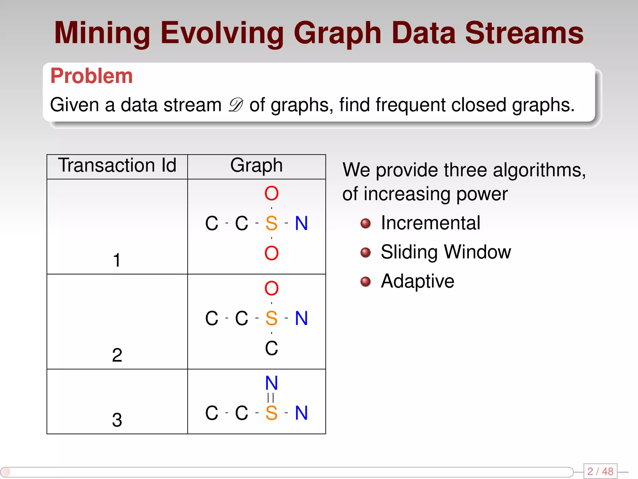
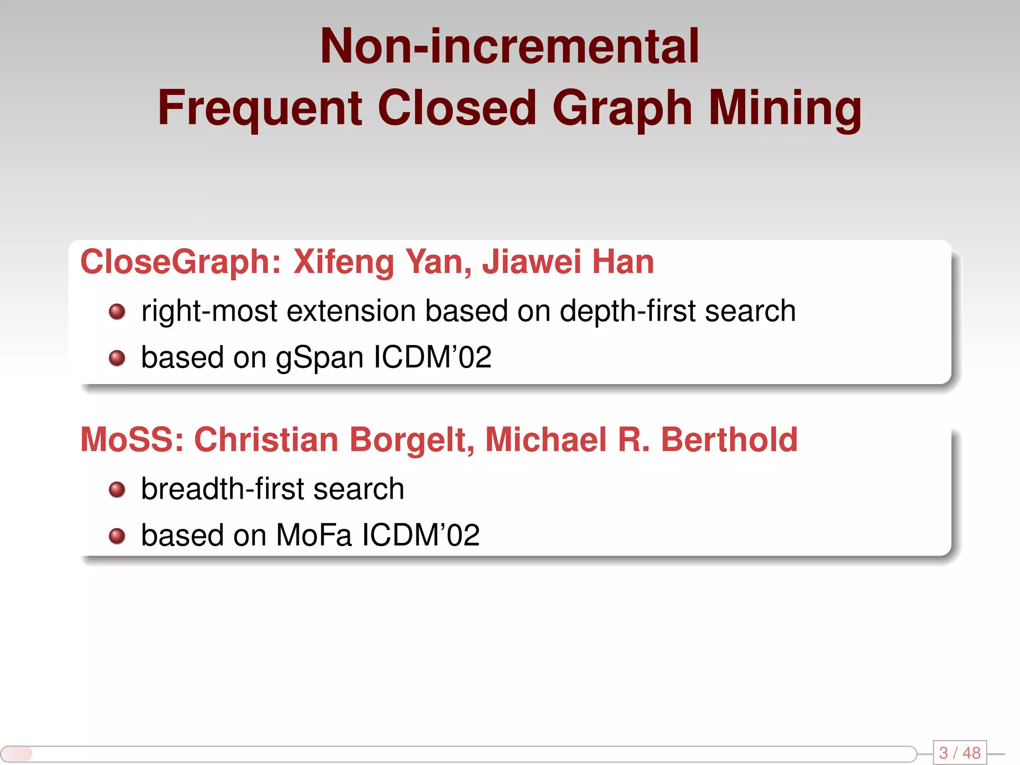
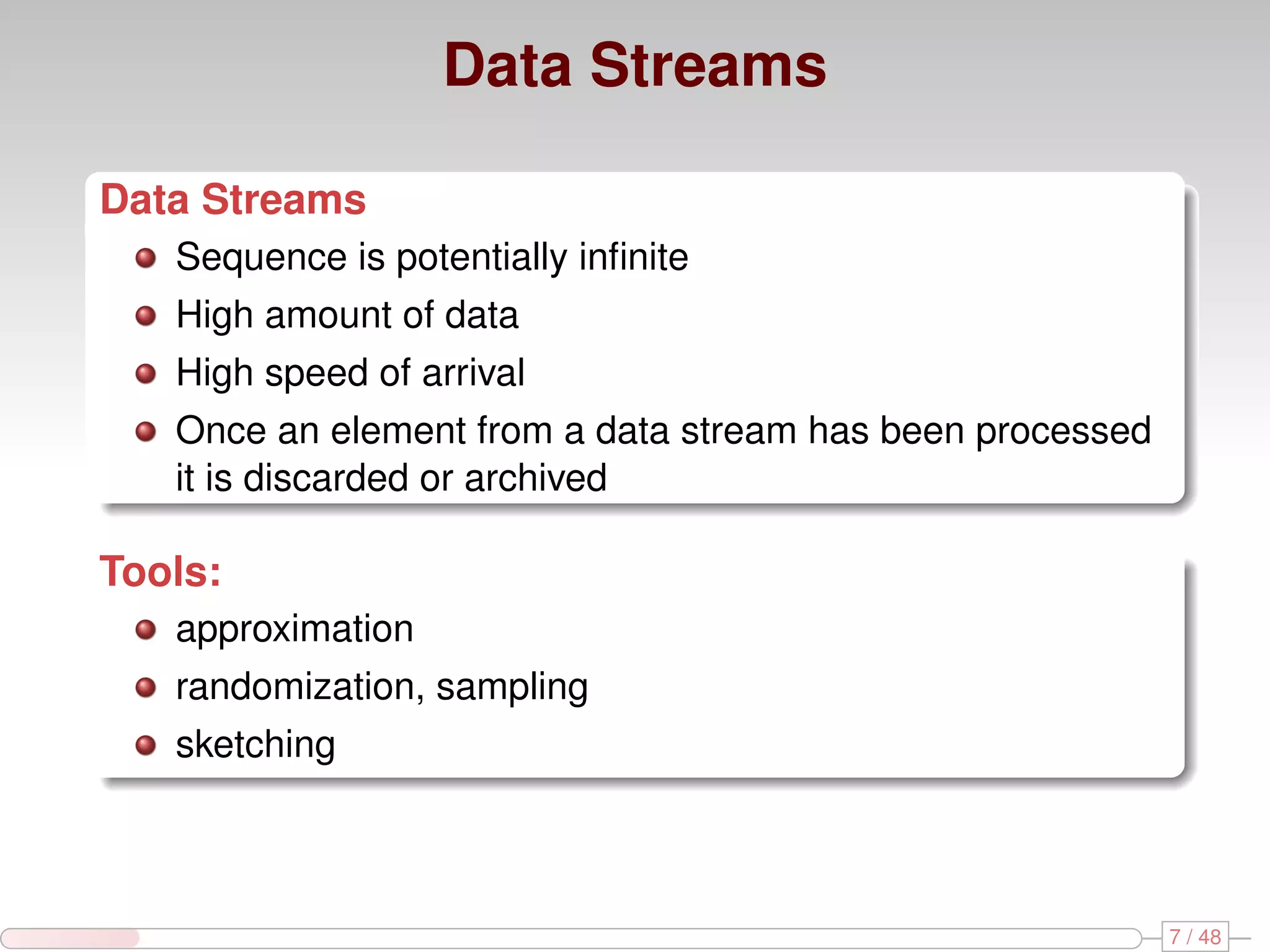
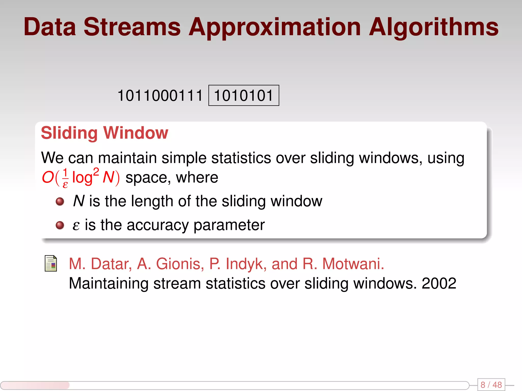
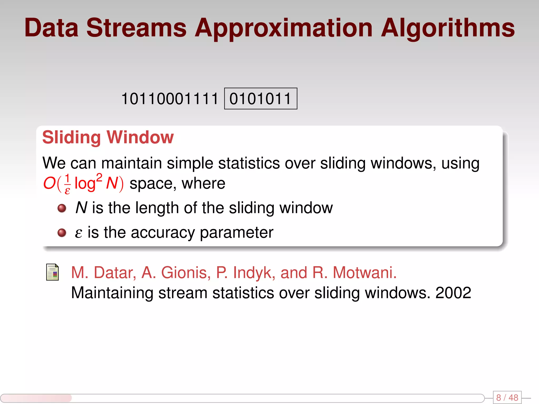
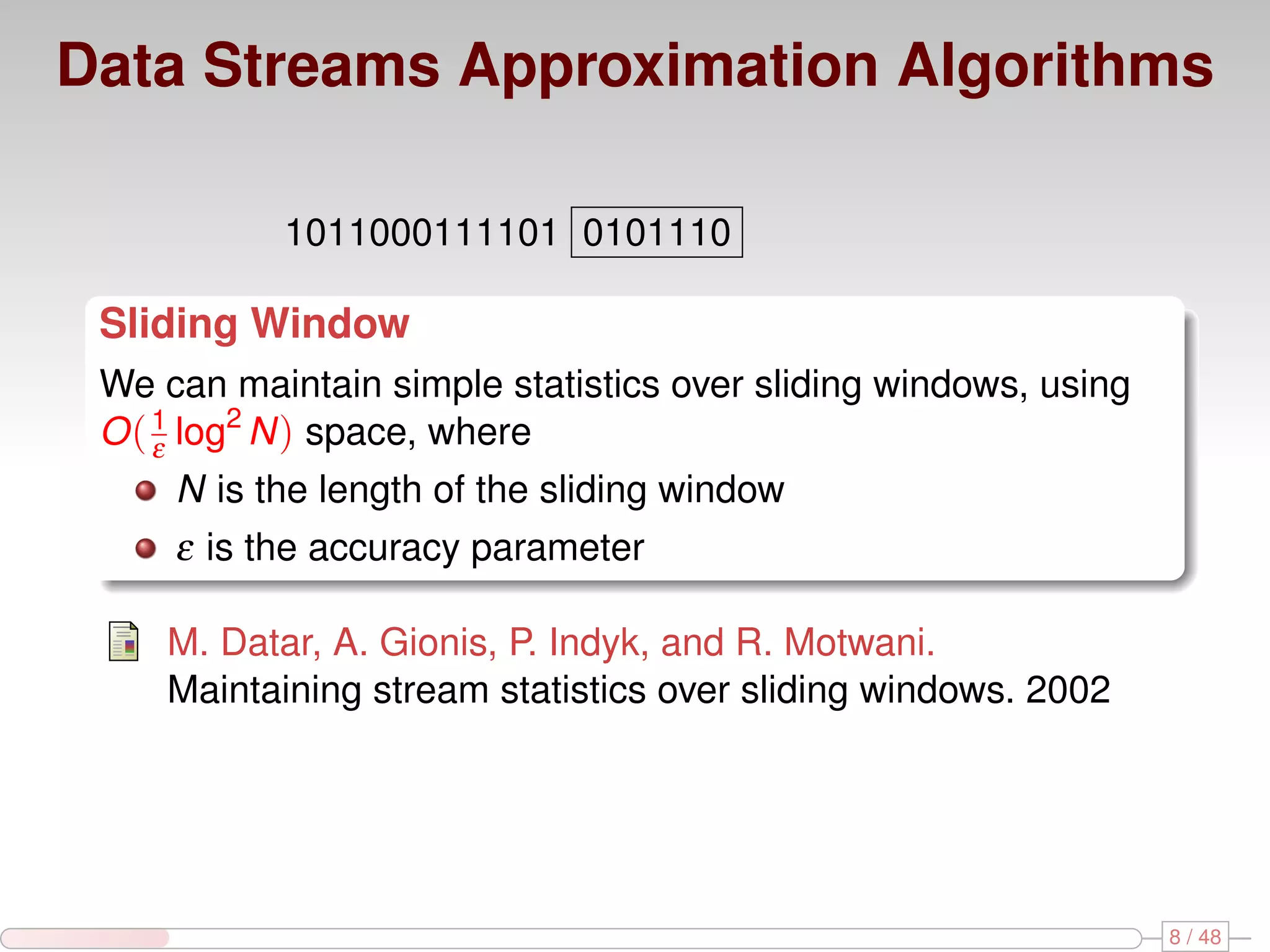
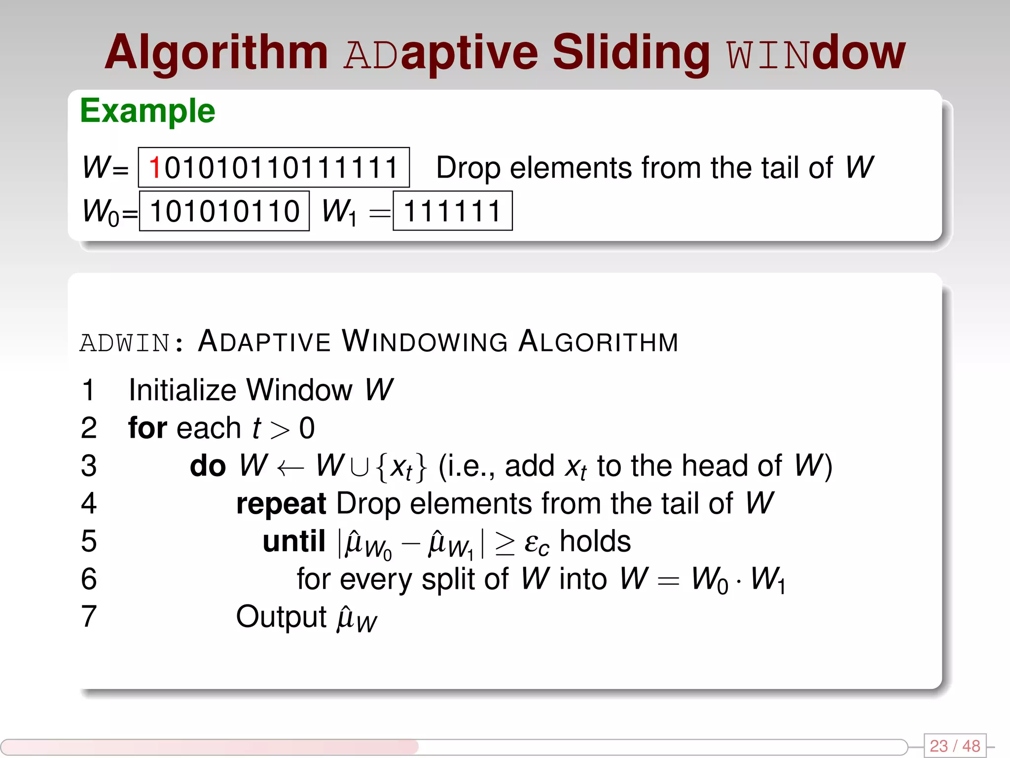
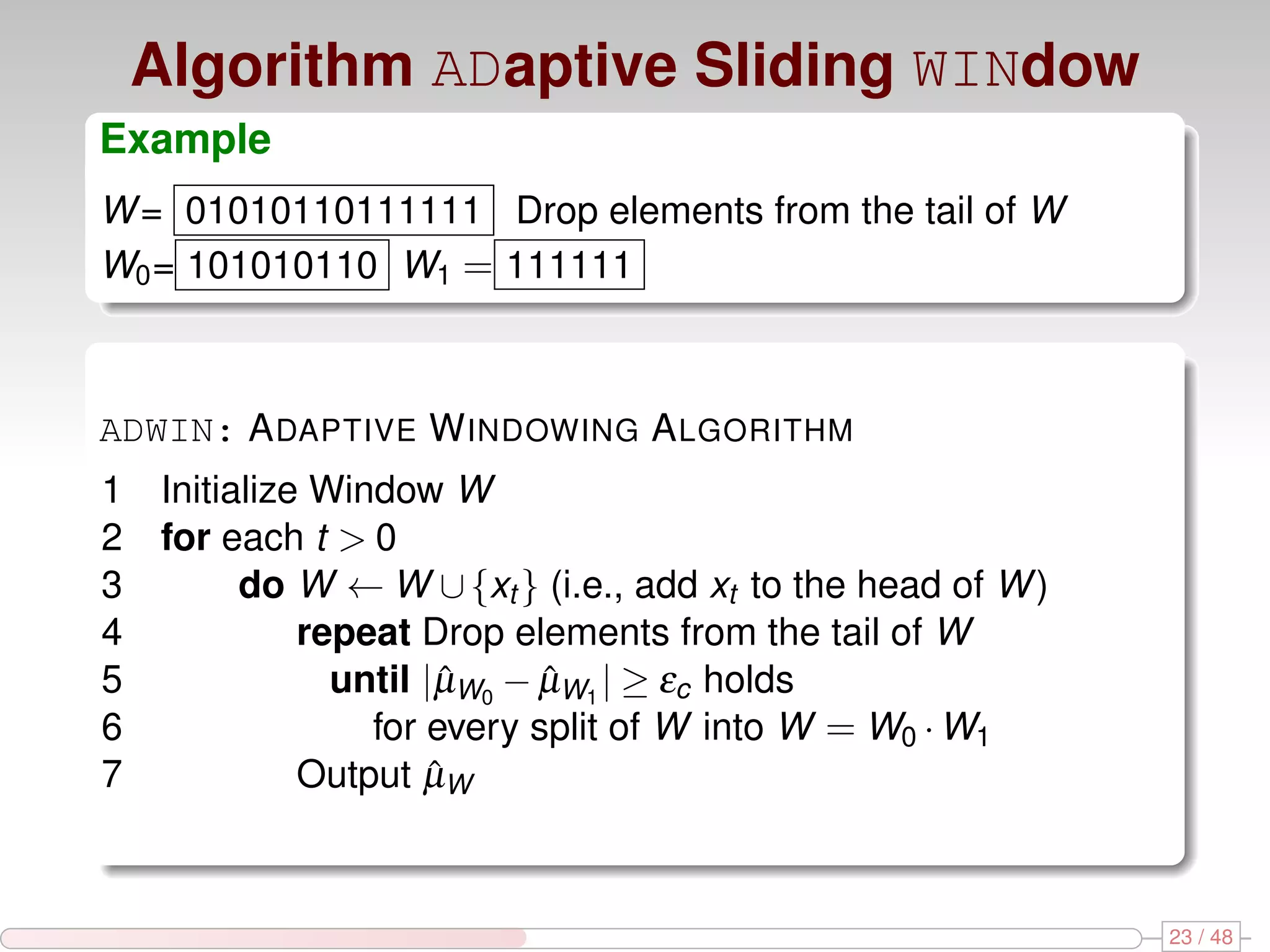
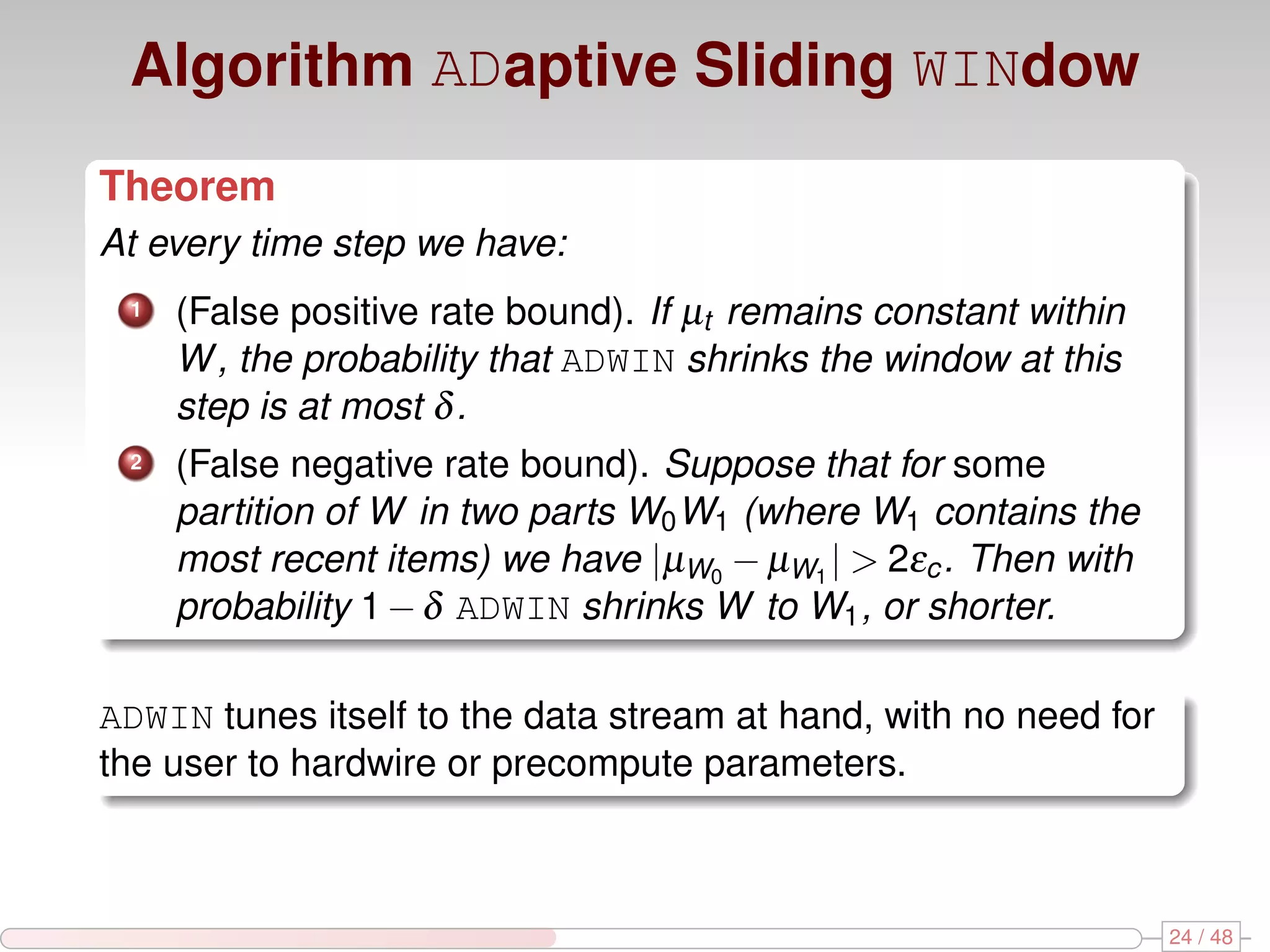
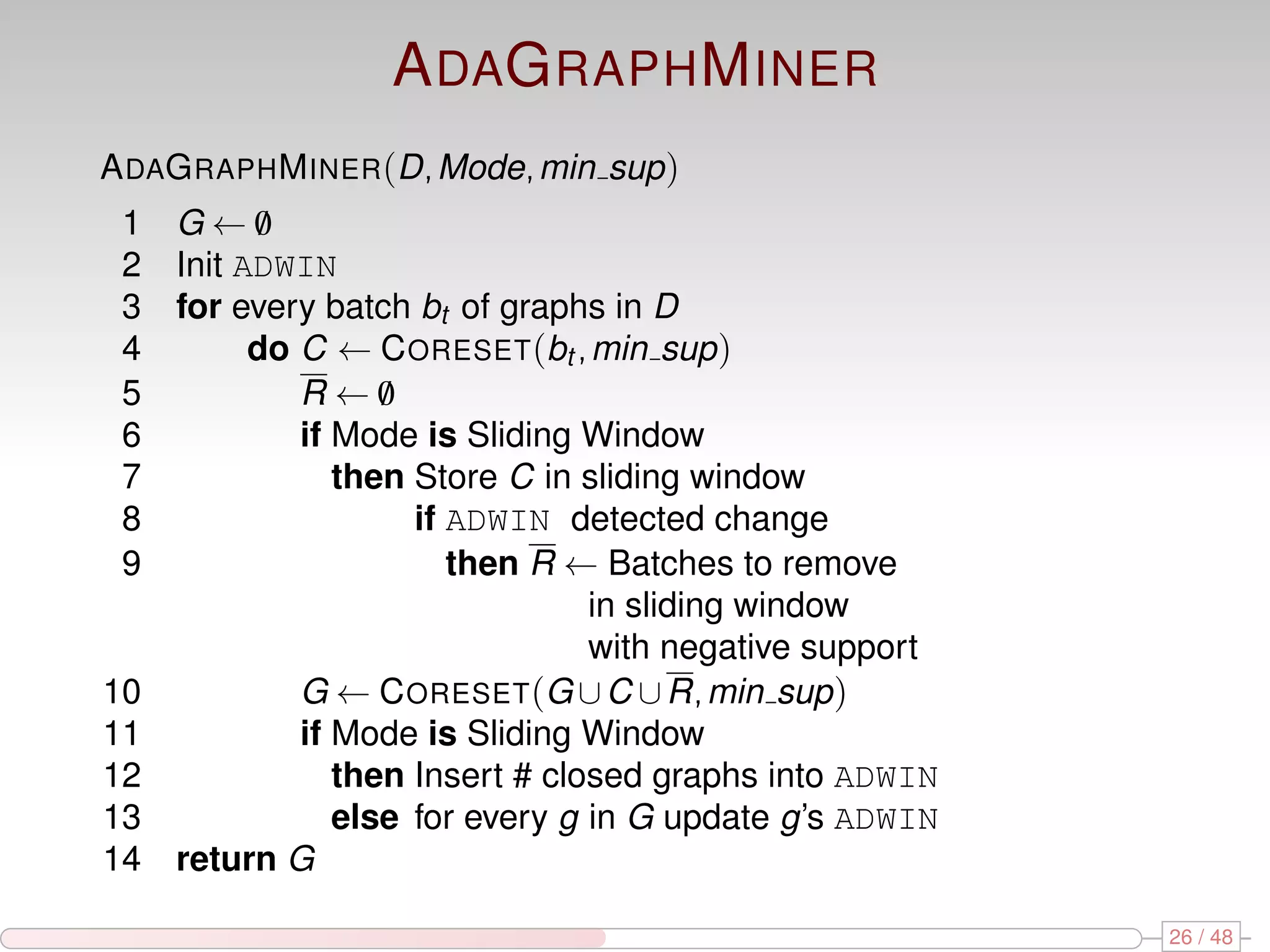
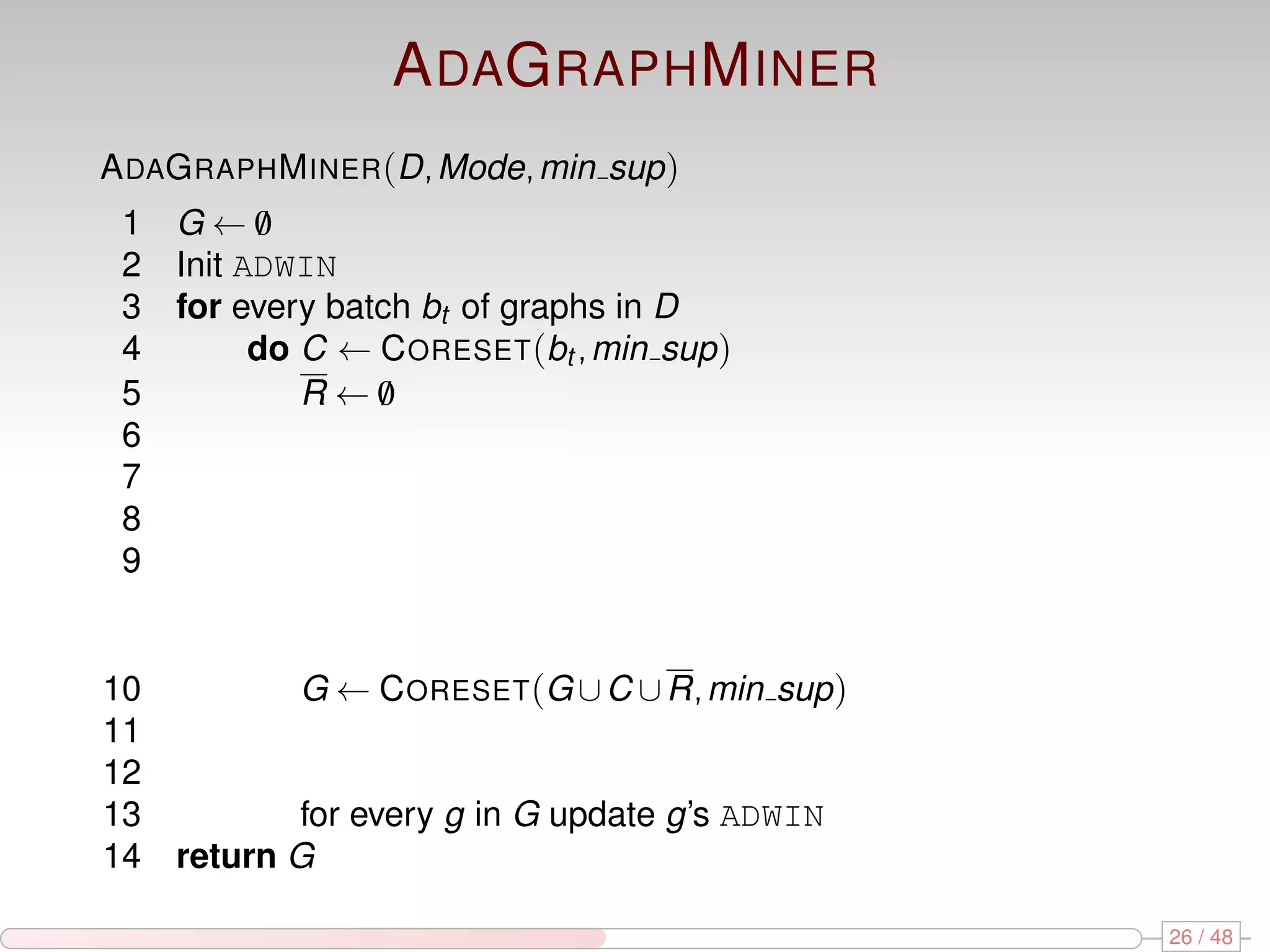
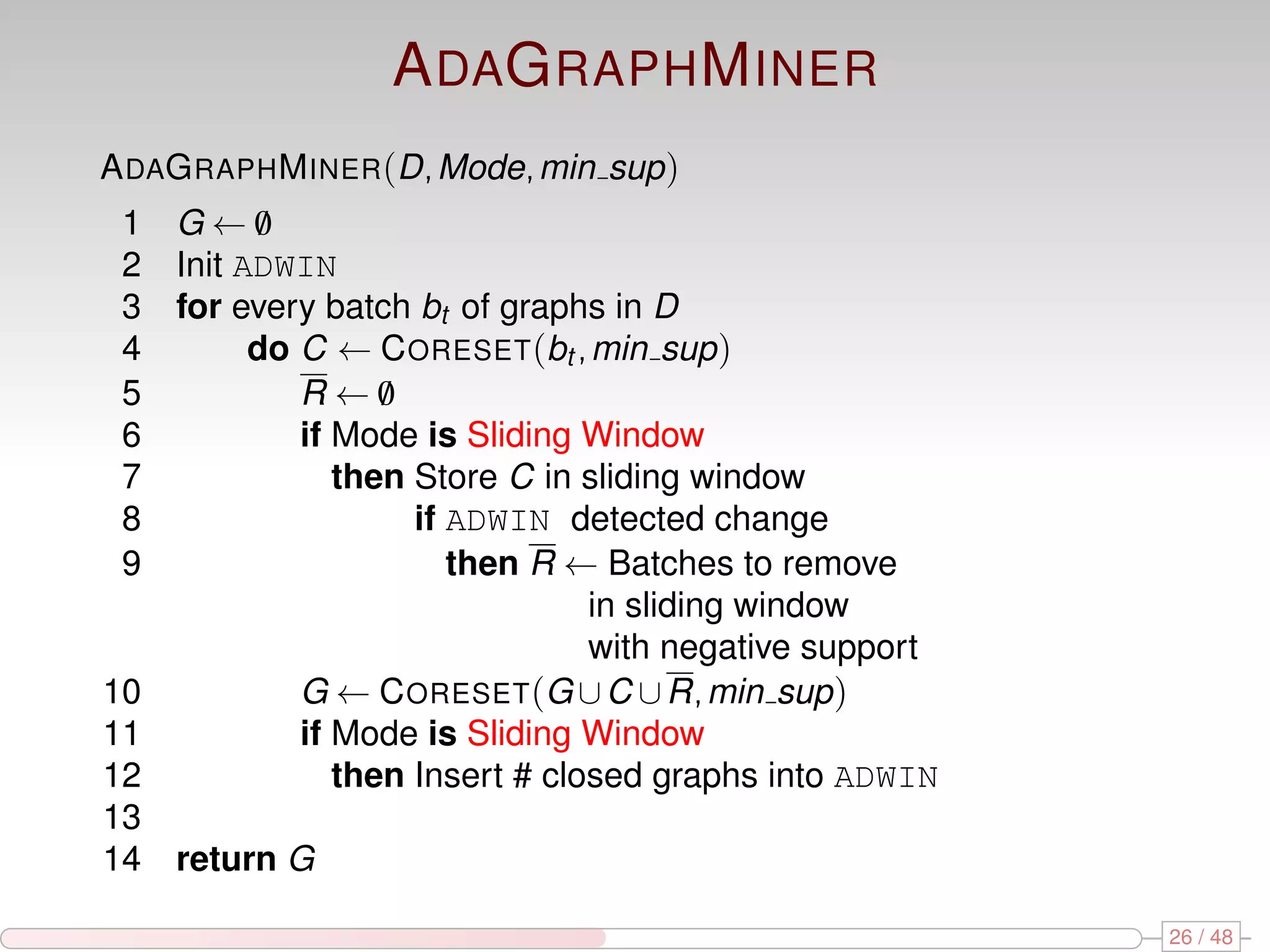
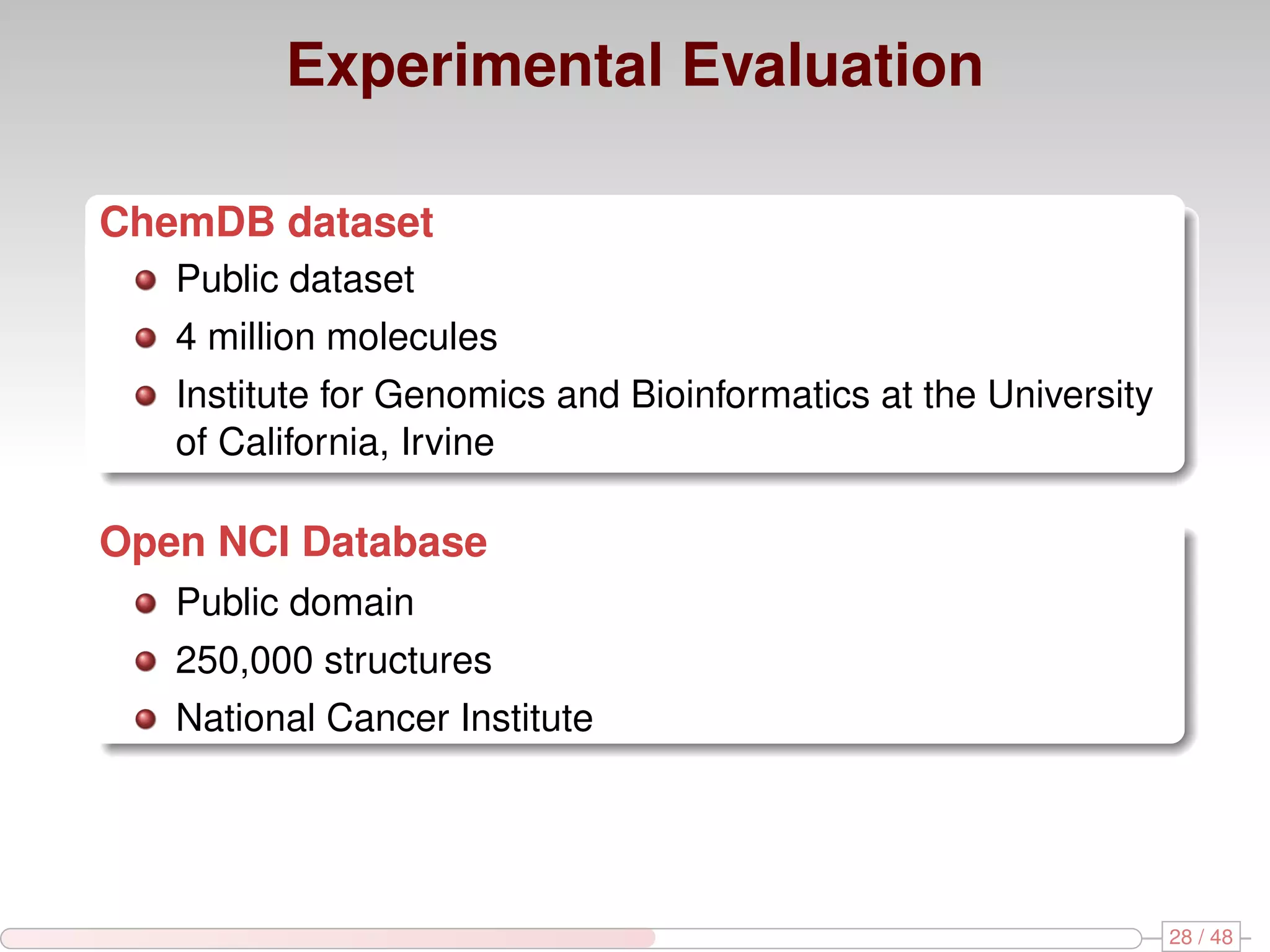
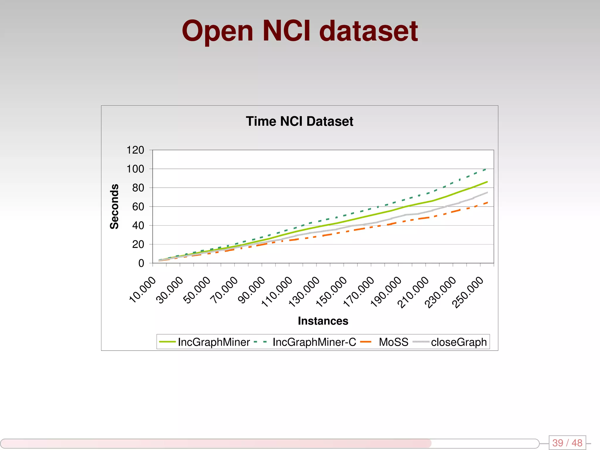
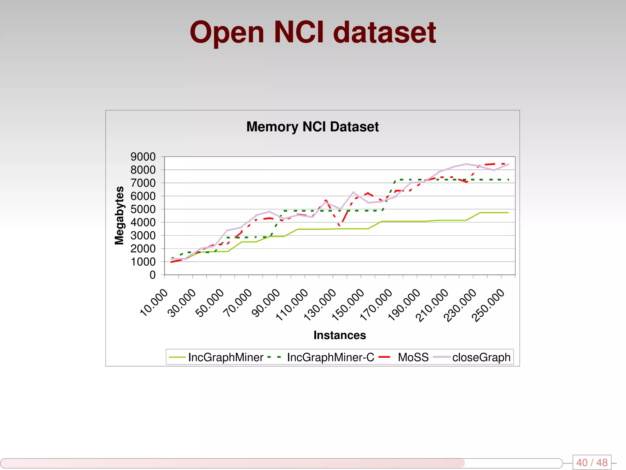
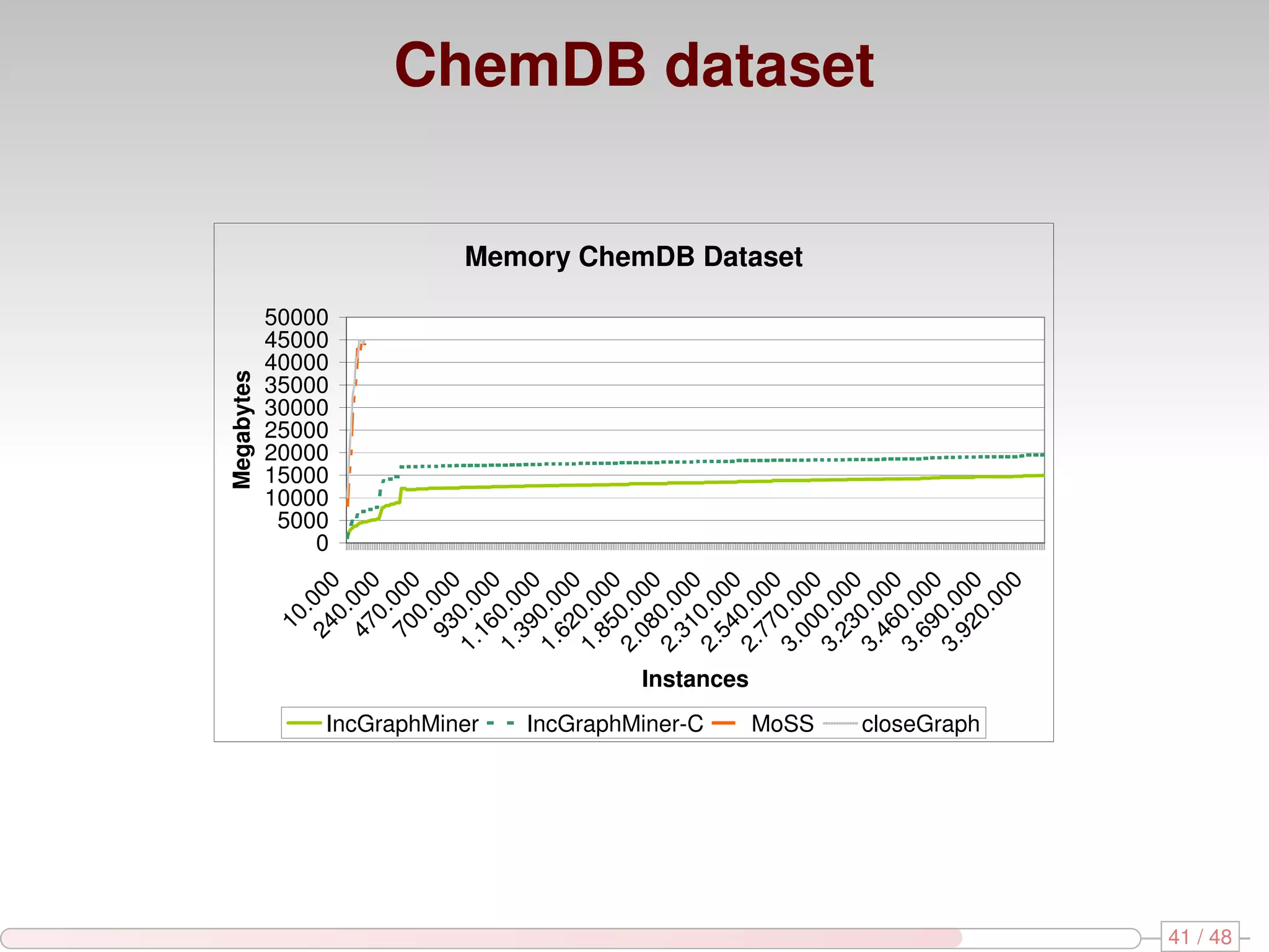
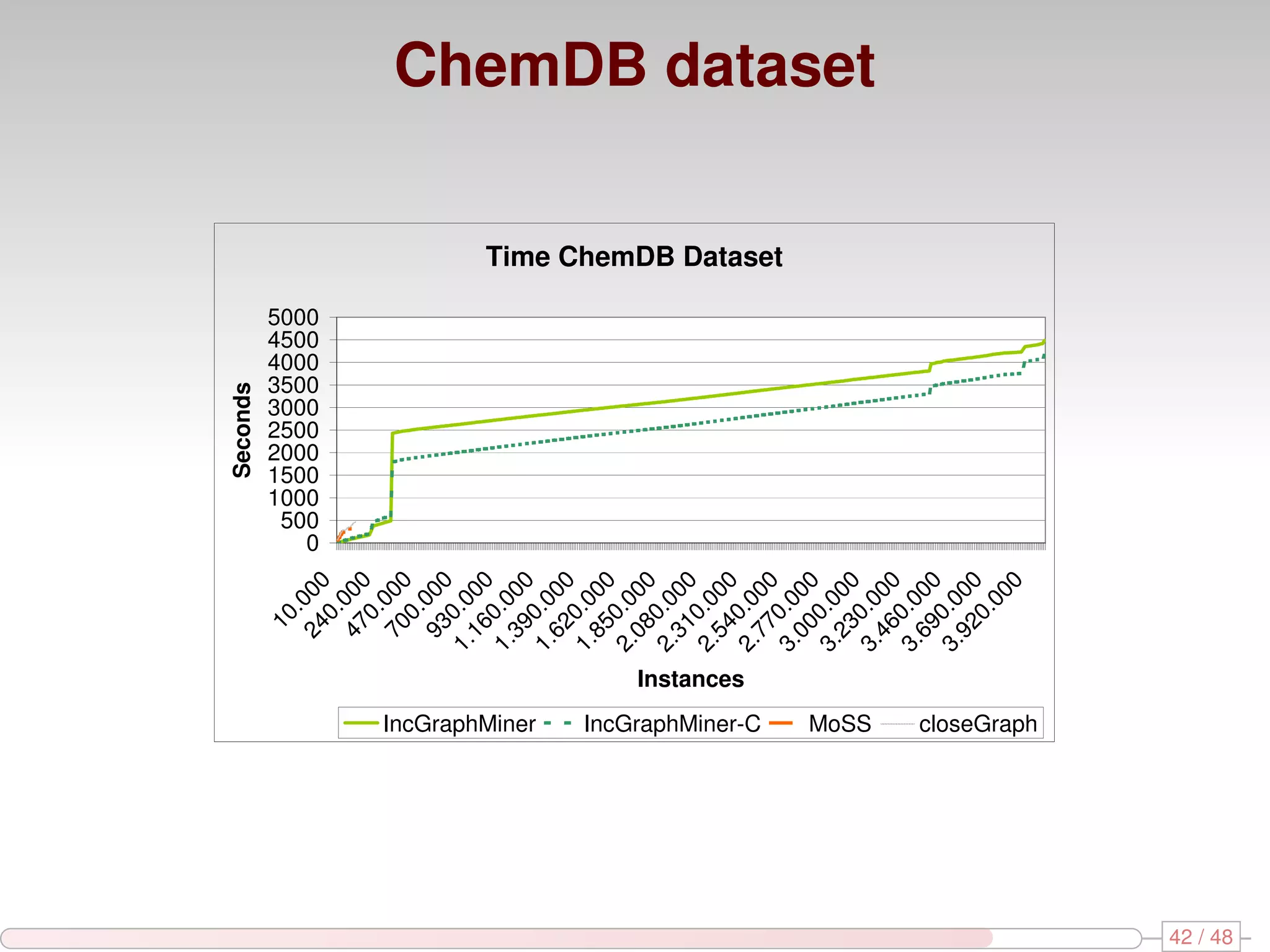
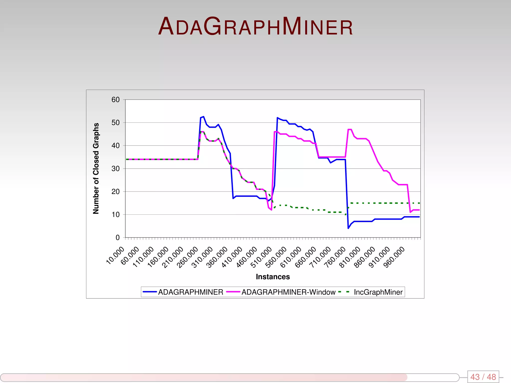
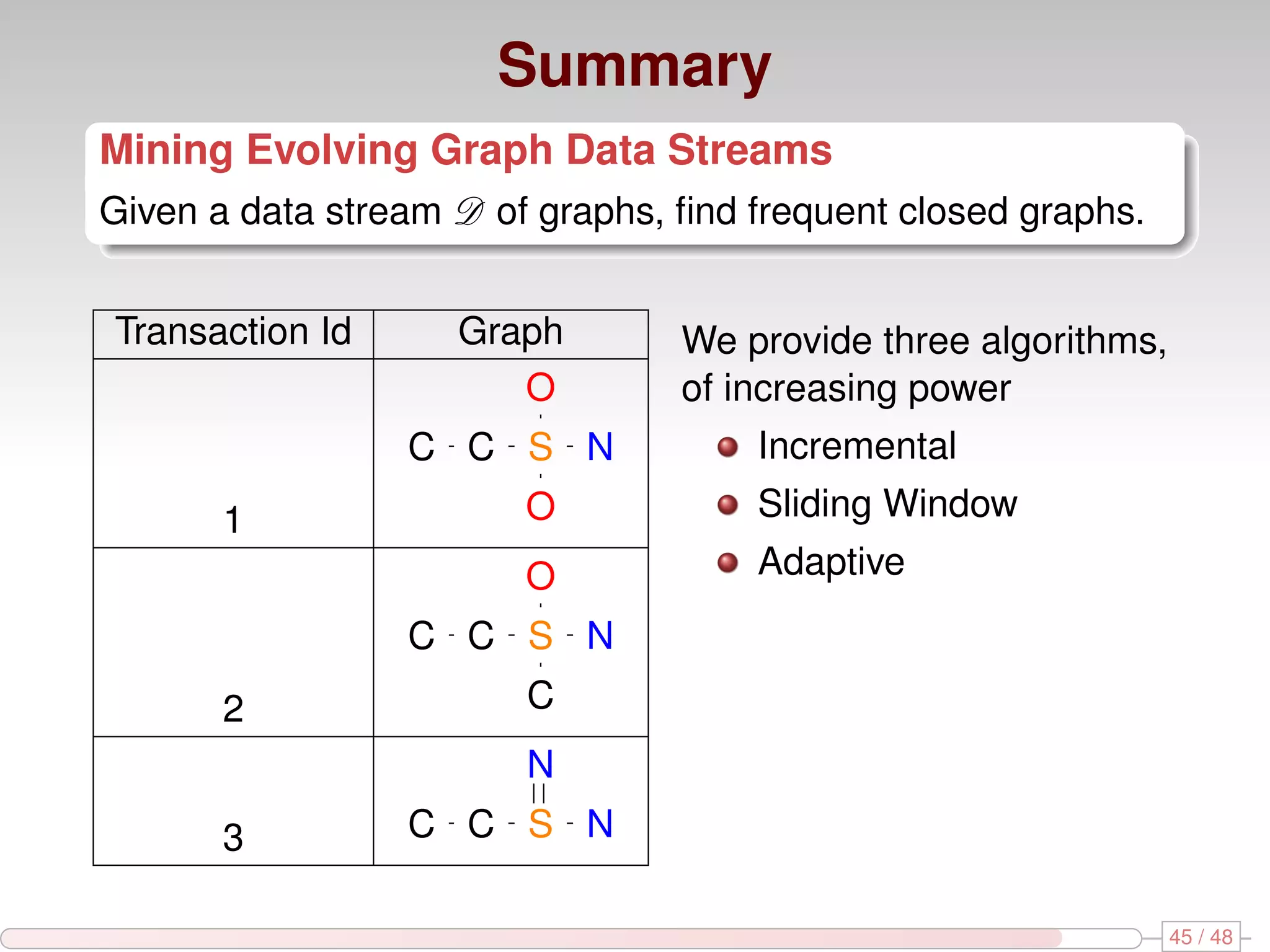
Mining Frequent Closed Graphs on Evolving Data Streams ` A. Bifet, G. Holmes, B. Pfahringer and R. Gavalda University of Waikato Hamilton, New Zealand Laboratory for Relational Algorithmics, Complexity and Learning LARCA UPC-Barcelona Tech, Catalonia San Diego, 24 August 2011 17th ACM SIGKDD International Conference on Knowledge Discovery and Data Mining 2011
Mining Evolving Graph Data Streams Problem Given a data stream D of graphs, find frequent closed graphs. Transaction Id Graph We provide three algorithms, O of increasing power C C S N Incremental 1 O Sliding Window O Adaptive C C S N 2 C N 3 C C S N 2 / 48
Non-incremental Frequent Closed Graph Mining CloseGraph: Xifeng Yan, Jiawei Han right-most extension based on depth-first search based on gSpan ICDM’02 MoSS: Christian Borgelt, Michael R. Berthold breadth-first search based on MoFa ICDM’02 3 / 48
Outline 1 Streaming Data 2 Frequent Pattern Mining Mining Evolving Graph Streams A DAG RAPH M INER 3 Experimental Evaluation 4 Summary and Future Work 4 / 48
Outline 1 Streaming Data 2 Frequent Pattern Mining Mining Evolving Graph Streams A DAG RAPH M INER 3 Experimental Evaluation 4 Summary and Future Work 5 / 48
Mining Massive Data Source: IDC’s Digital Universe Study (EMC), June 2011 6 / 48
Data Streams Data Streams Sequence is potentially infinite High amount of data High speed of arrival Once an element from a data stream has been processed it is discarded or archived Tools: approximation randomization, sampling sketching 7 / 48
Data Streams Approximation Algorithms 1011000111 1010101 Sliding Window We can maintain simple statistics over sliding windows, using O ( 1 log2 N ) space, where ε N is the length of the sliding window ε is the accuracy parameter M. Datar, A. Gionis, P. Indyk, and R. Motwani. Maintaining stream statistics over sliding windows. 2002 8 / 48
Data Streams Approximation Algorithms 10110001111 0101011 Sliding Window We can maintain simple statistics over sliding windows, using O ( 1 log2 N ) space, where ε N is the length of the sliding window ε is the accuracy parameter M. Datar, A. Gionis, P. Indyk, and R. Motwani. Maintaining stream statistics over sliding windows. 2002 8 / 48
Data Streams Approximation Algorithms 101100011110 1010111 Sliding Window We can maintain simple statistics over sliding windows, using O ( 1 log2 N ) space, where ε N is the length of the sliding window ε is the accuracy parameter M. Datar, A. Gionis, P. Indyk, and R. Motwani. Maintaining stream statistics over sliding windows. 2002 8 / 48
Data Streams Approximation Algorithms 1011000111101 0101110 Sliding Window We can maintain simple statistics over sliding windows, using O ( 1 log2 N ) space, where ε N is the length of the sliding window ε is the accuracy parameter M. Datar, A. Gionis, P. Indyk, and R. Motwani. Maintaining stream statistics over sliding windows. 2002 8 / 48
Data Streams Approximation Algorithms 10110001111010 1011101 Sliding Window We can maintain simple statistics over sliding windows, using O ( 1 log2 N ) space, where ε N is the length of the sliding window ε is the accuracy parameter M. Datar, A. Gionis, P. Indyk, and R. Motwani. Maintaining stream statistics over sliding windows. 2002 8 / 48
Data Streams Approximation Algorithms 101100011110101 0111010 Sliding Window We can maintain simple statistics over sliding windows, using O ( 1 log2 N ) space, where ε N is the length of the sliding window ε is the accuracy parameter M. Datar, A. Gionis, P. Indyk, and R. Motwani. Maintaining stream statistics over sliding windows. 2002 8 / 48
Outline 1 Streaming Data 2 Frequent Pattern Mining Mining Evolving Graph Streams A DAG RAPH M INER 3 Experimental Evaluation 4 Summary and Future Work 9 / 48
Pattern Mining Dataset Example Document Patterns d1 abce d2 cde d3 abce d4 acde d5 abcde d6 bcd 10 / 48
Itemset Mining d1 abce Support Frequent d2 cde d1,d2,d3,d4,d5,d6 c d3 abce d1,d2,d3,d4,d5 e,ce d4 acde d1,d3,d4,d5 a,ac,ae,ace d5 abcde d1,d3,d5,d6 b,bc d6 bcd d2,d4,d5 d,cd d1,d3,d5 ab,abc,abe be,bce,abce d2,d4,d5 de,cde 11 / 48
Itemset Mining d1 abce Support Frequent d2 cde 6 c d3 abce 5 e,ce d4 acde 4 a,ac,ae,ace d5 abcde 4 b,bc d6 bcd 4 d,cd 3 ab,abc,abe be,bce,abce 3 de,cde 12 / 48
Itemset Mining d1 abce Support Frequent Gen Closed d2 cde 6 c c c d3 abce 5 e,ce e ce d4 acde 4 a,ac,ae,ace a ace d5 abcde 4 b,bc b bc d6 bcd 4 d,cd d cd 3 ab,abc,abe ab be,bce,abce be abce 3 de,cde de cde 12 / 48
Itemset Mining d1 abce Support Frequent Gen Closed Max d2 cde 6 c c c d3 abce 5 e,ce e ce d4 acde 4 a,ac,ae,ace a ace d5 abcde 4 b,bc b bc d6 bcd 4 d,cd d cd 3 ab,abc,abe ab be,bce,abce be abce abce 3 de,cde de cde cde 12 / 48
Outline 1 Streaming Data 2 Frequent Pattern Mining Mining Evolving Graph Streams A DAG RAPH M INER 3 Experimental Evaluation 4 Summary and Future Work 13 / 48
Graph Dataset Transaction Id Graph Weight O C C S N 1 O 1 O C C S N 2 C 1 O C S N 3 C 1 N 4 C C S N 1 14 / 48
Graph Coresets Coreset of a set P with respect to some problem Small subset that approximates the original set P. Solving the problem for the coreset provides an approximate solution for the problem on P. δ -tolerance Closed Graph A graph g is δ -tolerance closed if none of its proper frequent supergraphs has a weighted support ≥ (1 − δ ) · support (g ). Maximal graph: 1-tolerance closed graph Closed graph: 0-tolerance closed graph. 15 / 48
Graph Coresets Relative support of a closed graph Support of a graph minus the relative support of its closed supergraphs. The sum of the closed supergraphs’ relative supports of a graph and its relative support is equal to its own support. (s, δ )-coreset for the problem of computing closed graphs Weighted multiset of frequent δ -tolerance closed graphs with minimum support s using their relative support as a weight. 16 / 48
Graph Dataset Transaction Id Graph Weight O C C S N 1 O 1 O C C S N 2 C 1 O C S N 3 C 1 N 4 C C S N 1 17 / 48
Graph Coresets Graph Relative Support Support C C S N 3 3 O C S N 3 3 N C S 3 3 Table: Example of a coreset with minimum support 50% and δ = 1 18 / 48
Graph Coresets Figure: Number of graphs in a (40%, δ )-coreset for NCI. 19 / 48
Outline 1 Streaming Data 2 Frequent Pattern Mining Mining Evolving Graph Streams A DAG RAPH M INER 3 Experimental Evaluation 4 Summary and Future Work 20 / 48
I NC G RAPH M INER I NC G RAPH M INER (D, min sup ) Input: A graph dataset D, and min sup. Output: The frequent graph set G. 1 G←0 / 2 for every batch bt of graphs in D 3 do C ← C ORESET (bt , min sup ) 4 G ← C ORESET (G ∪ C, min sup ) 5 return G 21 / 48
W IN G RAPH M INER W IN G RAPH M INER (D, W , min sup ) Input: A graph dataset D, a size window W and min sup. Output: The frequent graph set G. 1 G←0 / 2 for every batch bt of graphs in D 3 do C ← C ORESET (bt , min sup ) 4 Store C in sliding window 5 if sliding window is full 6 then R ← Oldest C stored in sliding window, negate all support values 7 else R ← 0 / 8 G ← C ORESET (G ∪ C ∪ R, min sup ) 9 return G 22 / 48
Algorithm ADaptive Sliding WINdow Example W = 101010110111111 W0 = 1 ADWIN: A DAPTIVE W INDOWING A LGORITHM 1 Initialize Window W 2 for each t > 0 3 do W ← W ∪ {xt } (i.e., add xt to the head of W ) 4 repeat Drop elements from the tail of W 5 until |µW0 − µW1 | ≥ εc holds ˆ ˆ 6 for every split of W into W = W0 · W1 7 Output µWˆ 23 / 48
Algorithm ADaptive Sliding WINdow Example W = 101010110111111 W0 = 1 W1 = 01010110111111 ADWIN: A DAPTIVE W INDOWING A LGORITHM 1 Initialize Window W 2 for each t > 0 3 do W ← W ∪ {xt } (i.e., add xt to the head of W ) 4 repeat Drop elements from the tail of W 5 until |µW0 − µW1 | ≥ εc holds ˆ ˆ 6 for every split of W into W = W0 · W1 7 Output µWˆ 23 / 48
Algorithm ADaptive Sliding WINdow Example W = 101010110111111 W0 = 10 W1 = 1010110111111 ADWIN: A DAPTIVE W INDOWING A LGORITHM 1 Initialize Window W 2 for each t > 0 3 do W ← W ∪ {xt } (i.e., add xt to the head of W ) 4 repeat Drop elements from the tail of W 5 until |µW0 − µW1 | ≥ εc holds ˆ ˆ 6 for every split of W into W = W0 · W1 7 Output µWˆ 23 / 48
Algorithm ADaptive Sliding WINdow Example W = 101010110111111 W0 = 101 W1 = 010110111111 ADWIN: A DAPTIVE W INDOWING A LGORITHM 1 Initialize Window W 2 for each t > 0 3 do W ← W ∪ {xt } (i.e., add xt to the head of W ) 4 repeat Drop elements from the tail of W 5 until |µW0 − µW1 | ≥ εc holds ˆ ˆ 6 for every split of W into W = W0 · W1 7 Output µWˆ 23 / 48
Algorithm ADaptive Sliding WINdow Example W = 101010110111111 W0 = 1010 W1 = 10110111111 ADWIN: A DAPTIVE W INDOWING A LGORITHM 1 Initialize Window W 2 for each t > 0 3 do W ← W ∪ {xt } (i.e., add xt to the head of W ) 4 repeat Drop elements from the tail of W 5 until |µW0 − µW1 | ≥ εc holds ˆ ˆ 6 for every split of W into W = W0 · W1 7 Output µWˆ 23 / 48
Algorithm ADaptive Sliding WINdow Example W = 101010110111111 W0 = 10101 W1 = 0110111111 ADWIN: A DAPTIVE W INDOWING A LGORITHM 1 Initialize Window W 2 for each t > 0 3 do W ← W ∪ {xt } (i.e., add xt to the head of W ) 4 repeat Drop elements from the tail of W 5 until |µW0 − µW1 | ≥ εc holds ˆ ˆ 6 for every split of W into W = W0 · W1 7 Output µWˆ 23 / 48
Algorithm ADaptive Sliding WINdow Example W = 101010110111111 W0 = 101010 W1 = 110111111 ADWIN: A DAPTIVE W INDOWING A LGORITHM 1 Initialize Window W 2 for each t > 0 3 do W ← W ∪ {xt } (i.e., add xt to the head of W ) 4 repeat Drop elements from the tail of W 5 until |µW0 − µW1 | ≥ εc holds ˆ ˆ 6 for every split of W into W = W0 · W1 7 Output µWˆ 23 / 48
Algorithm ADaptive Sliding WINdow Example W = 101010110111111 W0 = 1010101 W1 = 10111111 ADWIN: A DAPTIVE W INDOWING A LGORITHM 1 Initialize Window W 2 for each t > 0 3 do W ← W ∪ {xt } (i.e., add xt to the head of W ) 4 repeat Drop elements from the tail of W 5 until |µW0 − µW1 | ≥ εc holds ˆ ˆ 6 for every split of W into W = W0 · W1 7 Output µWˆ 23 / 48
Algorithm ADaptive Sliding WINdow Example W = 101010110111111 W0 = 10101011 W1 = 0111111 ADWIN: A DAPTIVE W INDOWING A LGORITHM 1 Initialize Window W 2 for each t > 0 3 do W ← W ∪ {xt } (i.e., add xt to the head of W ) 4 repeat Drop elements from the tail of W 5 until |µW0 − µW1 | ≥ εc holds ˆ ˆ 6 for every split of W into W = W0 · W1 7 Output µWˆ 23 / 48
Algorithm ADaptive Sliding WINdow Example W = 101010110111111 |µW0 − µW1 | ≥ εc : CHANGE DET.! ˆ ˆ W0 = 101010110 W1 = 111111 ADWIN: A DAPTIVE W INDOWING A LGORITHM 1 Initialize Window W 2 for each t > 0 3 do W ← W ∪ {xt } (i.e., add xt to the head of W ) 4 repeat Drop elements from the tail of W 5 until |µW0 − µW1 | ≥ εc holds ˆ ˆ 6 for every split of W into W = W0 · W1 7 Output µWˆ 23 / 48
Algorithm ADaptive Sliding WINdow Example W = 101010110111111 Drop elements from the tail of W W0 = 101010110 W1 = 111111 ADWIN: A DAPTIVE W INDOWING A LGORITHM 1 Initialize Window W 2 for each t > 0 3 do W ← W ∪ {xt } (i.e., add xt to the head of W ) 4 repeat Drop elements from the tail of W 5 until |µW0 − µW1 | ≥ εc holds ˆ ˆ 6 for every split of W into W = W0 · W1 7 Output µWˆ 23 / 48
Algorithm ADaptive Sliding WINdow Example W = 01010110111111 Drop elements from the tail of W W0 = 101010110 W1 = 111111 ADWIN: A DAPTIVE W INDOWING A LGORITHM 1 Initialize Window W 2 for each t > 0 3 do W ← W ∪ {xt } (i.e., add xt to the head of W ) 4 repeat Drop elements from the tail of W 5 until |µW0 − µW1 | ≥ εc holds ˆ ˆ 6 for every split of W into W = W0 · W1 7 Output µWˆ 23 / 48
Algorithm ADaptive Sliding WINdow Theorem At every time step we have: 1 (False positive rate bound). If µt remains constant within W , the probability that ADWIN shrinks the window at this step is at most δ . 2 (False negative rate bound). Suppose that for some partition of W in two parts W0 W1 (where W1 contains the most recent items) we have |µW0 − µW1 | > 2εc . Then with probability 1 − δ ADWIN shrinks W to W1 , or shorter. ADWIN tunes itself to the data stream at hand, with no need for the user to hardwire or precompute parameters. 24 / 48
Algorithm ADaptive Sliding WINdow ADWIN using a Data Stream Sliding Window Model, can provide the exact counts of 1’s in O (1) time per point. tries O (log W ) cutpoints uses O ( 1 log W ) memory words ε the processing time per example is O (log W ) (amortized and worst-case). Sliding Window Model 1010101 101 11 1 1 Content: 4 2 2 1 1 Capacity: 7 3 2 1 1 25 / 48
A DAG RAPH M INER A DAG RAPH M INER (D, Mode, min sup ) 1 G←0 / 2 Init ADWIN 3 for every batch bt of graphs in D 4 do C ← C ORESET (bt , min sup ) 5 R←0 / 6 if Mode is Sliding Window 7 then Store C in sliding window 8 if ADWIN detected change 9 then R ← Batches to remove in sliding window with negative support 10 G ← C ORESET (G ∪ C ∪ R, min sup ) 11 if Mode is Sliding Window 12 then Insert # closed graphs into ADWIN 13 else for every g in G update g’s ADWIN 14 return G 26 / 48
A DAG RAPH M INER A DAG RAPH M INER (D, Mode, min sup ) 1 G←0 / 2 Init ADWIN 3 for every batch bt of graphs in D 4 do C ← C ORESET (bt , min sup ) 5 R←0 / 6 7 8 9 10 G ← C ORESET (G ∪ C ∪ R, min sup ) 11 12 13 for every g in G update g’s ADWIN 14 return G 26 / 48
A DAG RAPH M INER A DAG RAPH M INER (D, Mode, min sup ) 1 G←0 / 2 Init ADWIN 3 for every batch bt of graphs in D 4 do C ← C ORESET (bt , min sup ) 5 R←0 / 6 if Mode is Sliding Window 7 then Store C in sliding window 8 if ADWIN detected change 9 then R ← Batches to remove in sliding window with negative support 10 G ← C ORESET (G ∪ C ∪ R, min sup ) 11 if Mode is Sliding Window 12 then Insert # closed graphs into ADWIN 13 14 return G 26 / 48
Outline 1 Streaming Data 2 Frequent Pattern Mining Mining Evolving Graph Streams A DAG RAPH M INER 3 Experimental Evaluation 4 Summary and Future Work 27 / 48
Experimental Evaluation ChemDB dataset Public dataset 4 million molecules Institute for Genomics and Bioinformatics at the University of California, Irvine Open NCI Database Public domain 250,000 structures National Cancer Institute 28 / 48
What is MOA? {M}assive {O}nline {A}nalysis is a framework for online learning from data streams. It is closely related to WEKA It includes a collection of offline and online as well as tools for evaluation: classification clustering Easy to extend Easy to design and run experiments 29 / 48
WEKA: the bird 30 / 48
MOA: the bird The Moa (another native NZ bird) is not only flightless, like the Weka, but also extinct. 31 / 48
Classification Experimental Setting 32 / 48
Classification Experimental Setting Classifiers Naive Bayes Decision stumps Hoeffding Tree Hoeffding Option Tree Bagging and Boosting ADWIN Bagging and Leveraging Bagging Prediction strategies Majority class Naive Bayes Leaves Adaptive Hybrid 33 / 48
Clustering Experimental Setting 34 / 48
Clustering Experimental Setting Clusterers StreamKM++ CluStream ClusTree Den-Stream CobWeb 35 / 48
Clustering Experimental Setting Internal measures External measures Gamma Rand statistic C Index Jaccard coefficient Point-Biserial Folkes and Mallow Index Log Likelihood Hubert Γ statistics Dunn’s Index Minkowski score Tau Purity Tau A van Dongen criterion Tau C V-measure Somer’s Gamma Completeness Ratio of Repetition Homogeneity Modified Ratio of Repetition Variation of information Adjusted Ratio of Clustering Mutual information Fagan’s Index Class-based entropy Deviation Index Cluster-based entropy Z-Score Index Precision D Index Recall Silhouette coefficient F-measure Table: Internal and external clustering evaluation measures. 36 / 48
Cluster Mapping Measure Hardy Kremer, Philipp Kranen, Timm Jansen, Thomas Seidl, Albert Bifet, Geoff Holmes and Bernhard Pfahringer. An Effective Evaluation Measure for Clustering on Evolving Data Stream KDD’11 CMM: Cluster Mapping Measure A novel evaluation measure for stream clustering on evolving streams ∑o∈F w (o ) · pen(o, C ) CMM (C , C L ) = 1 − ∑o∈F w (o ) · con(o, Cl (o )) 37 / 48
Extensions of MOA Multi-label Classification Active Learning Regression Closed Frequent Graph Mining Twitter Sentiment Analysis Challenges for bigger data streams Sampling and distributed systems (Map-Reduce, Hadoop, S4) 38 / 48
Open NCI dataset Time NCI Dataset 120 100 80 Seconds 60 40 20 0 00 00 00 00 00 0 0 0 0 0 0 0 0 00 00 00 00 00 00 00 00 .0 .0 .0 .0 .0 0. 0. 0. 0. 0. 0. 0. 0. 10 30 50 70 90 11 13 15 17 19 21 23 25 Instances IncGraphMiner IncGraphMiner-C MoSS closeGraph 39 / 48
Open NCI dataset Memory NCI Dataset 9000 8000 7000 Megabytes 6000 5000 4000 3000 2000 1000 0 00 00 00 00 00 0 0 0 0 0 0 0 0 00 00 00 00 00 00 00 00 .0 .0 .0 .0 .0 0. 0. 0. 0. 0. 0. 0. 0. 10 30 50 70 90 11 13 15 17 19 21 23 25 Instances IncGraphMiner IncGraphMiner-C MoSS closeGraph 40 / 48
Megabytes 10 . 0 5000 10000 15000 20000 25000 30000 35000 40000 45000 24 000 50000 0. 47 000 0. 70 000 0. 93 000 IncGraphMiner 1. 0. 0 16 00 1. 0.0 39 00 1. 0.0 62 00 1. 0.0 85 00 2. 0.0 08 00 2. 0.0 31 00 IncGraphMiner-C 2. 0.0 54 00 Instances 2. 0.0 77 00 Memory ChemDB Dataset 3. 0.0 MoSS 00 00 3. 0.0 23 00 ChemDB dataset 3. 0.0 46 00 3. 0.0 69 00 3. 0.0 92 00 closeGraph 0. 00 0 41 / 48
Seconds 10 . 0 500 1000 1500 2000 2500 3000 3500 4000 4500 5000 24 000 0. 47 000 0. 70 000 0. 93 000 1. 0. 0 16 00 1. 0.0 39 00 IncGraphMiner 1. 0.0 62 00 1. 0.0 85 00 2. 0.0 08 00 2. 0.0 31 00 2. 0.0 54 00 Instances IncGraphMiner-C 2. 0.0 77 00 Time ChemDB Dataset 3. 0.0 00 00 3. 0.0 23 00 MoSS ChemDB dataset 3. 0.0 46 00 3. 0.0 69 00 3. 0.0 92 00 0. 00 0 closeGraph 42 / 48
Number of Closed Graphs 10 .0 0 10 20 30 40 50 60 0 60 0 .0 11 00 0. 0 16 00 0. 00 21 0 0. 0 26 00 0. 0 31 00 0. 0 36 00 0. 0 ADAGRAPHMINER 41 00 0. 0 46 00 0. 0 51 00 0. 0 56 00 0. 00 Instances 61 0 0. 0 66 00 0. 0 71 00 0. 0 76 00 ADAGRAPHMINER-Window 0. 0 81 00 0. A DAG RAPH M INER 0 86 00 0. 0 91 00 0. 0 96 00 0. 00 IncGraphMiner 0 43 / 48
Outline 1 Streaming Data 2 Frequent Pattern Mining Mining Evolving Graph Streams A DAG RAPH M INER 3 Experimental Evaluation 4 Summary and Future Work 44 / 48
Summary Mining Evolving Graph Data Streams Given a data stream D of graphs, find frequent closed graphs. Transaction Id Graph We provide three algorithms, O of increasing power C C S N Incremental 1 O Sliding Window O Adaptive C C S N 2 C N 3 C C S N 45 / 48
Summary {M}assive {O}nline {A}nalysis is a framework for online learning from data streams. http://moa.cs.waikato.ac.nz It is closely related to WEKA It includes a collection of offline and online as well as tools for evaluation: classification clustering frequent pattern mining MOA deals with evolving data streams MOA is easy to use and extend 46 / 48
Future work Structured massive data mining sampling, sketching parallel techniques 47 / 48
Thanks! 48 / 48

Mining Frequent Closed Graphs on Evolving Data Streams

  • 1.
    Mining Frequent ClosedGraphs on Evolving Data Streams ` A. Bifet, G. Holmes, B. Pfahringer and R. Gavalda University of Waikato Hamilton, New Zealand Laboratory for Relational Algorithmics, Complexity and Learning LARCA UPC-Barcelona Tech, Catalonia San Diego, 24 August 2011 17th ACM SIGKDD International Conference on Knowledge Discovery and Data Mining 2011
  • 2.
    Mining Evolving GraphData Streams Problem Given a data stream D of graphs, find frequent closed graphs. Transaction Id Graph We provide three algorithms, O of increasing power C C S N Incremental 1 O Sliding Window O Adaptive C C S N 2 C N 3 C C S N 2 / 48
  • 3.
    Non-incremental Frequent Closed Graph Mining CloseGraph: Xifeng Yan, Jiawei Han right-most extension based on depth-first search based on gSpan ICDM’02 MoSS: Christian Borgelt, Michael R. Berthold breadth-first search based on MoFa ICDM’02 3 / 48
  • 4.
    Outline 1 Streaming Data 2 Frequent Pattern Mining Mining Evolving Graph Streams A DAG RAPH M INER 3 Experimental Evaluation 4 Summary and Future Work 4 / 48
  • 5.
    Outline 1 Streaming Data 2 Frequent Pattern Mining Mining Evolving Graph Streams A DAG RAPH M INER 3 Experimental Evaluation 4 Summary and Future Work 5 / 48
  • 6.
    Mining Massive Data Source:IDC’s Digital Universe Study (EMC), June 2011 6 / 48
  • 7.
    Data Streams Data Streams Sequence is potentially infinite High amount of data High speed of arrival Once an element from a data stream has been processed it is discarded or archived Tools: approximation randomization, sampling sketching 7 / 48
  • 8.
    Data Streams ApproximationAlgorithms 1011000111 1010101 Sliding Window We can maintain simple statistics over sliding windows, using O ( 1 log2 N ) space, where ε N is the length of the sliding window ε is the accuracy parameter M. Datar, A. Gionis, P. Indyk, and R. Motwani. Maintaining stream statistics over sliding windows. 2002 8 / 48
  • 9.
    Data Streams ApproximationAlgorithms 10110001111 0101011 Sliding Window We can maintain simple statistics over sliding windows, using O ( 1 log2 N ) space, where ε N is the length of the sliding window ε is the accuracy parameter M. Datar, A. Gionis, P. Indyk, and R. Motwani. Maintaining stream statistics over sliding windows. 2002 8 / 48
  • 10.
    Data Streams ApproximationAlgorithms 101100011110 1010111 Sliding Window We can maintain simple statistics over sliding windows, using O ( 1 log2 N ) space, where ε N is the length of the sliding window ε is the accuracy parameter M. Datar, A. Gionis, P. Indyk, and R. Motwani. Maintaining stream statistics over sliding windows. 2002 8 / 48
  • 11.
    Data Streams ApproximationAlgorithms 1011000111101 0101110 Sliding Window We can maintain simple statistics over sliding windows, using O ( 1 log2 N ) space, where ε N is the length of the sliding window ε is the accuracy parameter M. Datar, A. Gionis, P. Indyk, and R. Motwani. Maintaining stream statistics over sliding windows. 2002 8 / 48
  • 12.
    Data Streams ApproximationAlgorithms 10110001111010 1011101 Sliding Window We can maintain simple statistics over sliding windows, using O ( 1 log2 N ) space, where ε N is the length of the sliding window ε is the accuracy parameter M. Datar, A. Gionis, P. Indyk, and R. Motwani. Maintaining stream statistics over sliding windows. 2002 8 / 48
  • 13.
    Data Streams ApproximationAlgorithms 101100011110101 0111010 Sliding Window We can maintain simple statistics over sliding windows, using O ( 1 log2 N ) space, where ε N is the length of the sliding window ε is the accuracy parameter M. Datar, A. Gionis, P. Indyk, and R. Motwani. Maintaining stream statistics over sliding windows. 2002 8 / 48
  • 14.
    Outline 1 Streaming Data 2 Frequent Pattern Mining Mining Evolving Graph Streams A DAG RAPH M INER 3 Experimental Evaluation 4 Summary and Future Work 9 / 48
  • 15.
    Pattern Mining Dataset Example Document Patterns d1 abce d2 cde d3 abce d4 acde d5 abcde d6 bcd 10 / 48
  • 16.
    Itemset Mining d1 abce Support Frequent d2 cde d1,d2,d3,d4,d5,d6 c d3 abce d1,d2,d3,d4,d5 e,ce d4 acde d1,d3,d4,d5 a,ac,ae,ace d5 abcde d1,d3,d5,d6 b,bc d6 bcd d2,d4,d5 d,cd d1,d3,d5 ab,abc,abe be,bce,abce d2,d4,d5 de,cde 11 / 48
  • 17.
    Itemset Mining d1 abce Support Frequent d2 cde 6 c d3 abce 5 e,ce d4 acde 4 a,ac,ae,ace d5 abcde 4 b,bc d6 bcd 4 d,cd 3 ab,abc,abe be,bce,abce 3 de,cde 12 / 48
  • 18.
    Itemset Mining d1 abce Support Frequent Gen Closed d2 cde 6 c c c d3 abce 5 e,ce e ce d4 acde 4 a,ac,ae,ace a ace d5 abcde 4 b,bc b bc d6 bcd 4 d,cd d cd 3 ab,abc,abe ab be,bce,abce be abce 3 de,cde de cde 12 / 48
  • 19.
    Itemset Mining d1 abce Support Frequent Gen Closed Max d2 cde 6 c c c d3 abce 5 e,ce e ce d4 acde 4 a,ac,ae,ace a ace d5 abcde 4 b,bc b bc d6 bcd 4 d,cd d cd 3 ab,abc,abe ab be,bce,abce be abce abce 3 de,cde de cde cde 12 / 48
  • 20.
    Outline 1 Streaming Data 2 Frequent Pattern Mining Mining Evolving Graph Streams A DAG RAPH M INER 3 Experimental Evaluation 4 Summary and Future Work 13 / 48
  • 21.
    Graph Dataset Transaction Id Graph Weight O C C S N 1 O 1 O C C S N 2 C 1 O C S N 3 C 1 N 4 C C S N 1 14 / 48
  • 22.
    Graph Coresets Coreset ofa set P with respect to some problem Small subset that approximates the original set P. Solving the problem for the coreset provides an approximate solution for the problem on P. δ -tolerance Closed Graph A graph g is δ -tolerance closed if none of its proper frequent supergraphs has a weighted support ≥ (1 − δ ) · support (g ). Maximal graph: 1-tolerance closed graph Closed graph: 0-tolerance closed graph. 15 / 48
  • 23.
    Graph Coresets Coreset ofa set P with respect to some problem Small subset that approximates the original set P. Solving the problem for the coreset provides an approximate solution for the problem on P. δ -tolerance Closed Graph A graph g is δ -tolerance closed if none of its proper frequent supergraphs has a weighted support ≥ (1 − δ ) · support (g ). Maximal graph: 1-tolerance closed graph Closed graph: 0-tolerance closed graph. 15 / 48
  • 24.
    Graph Coresets Relative supportof a closed graph Support of a graph minus the relative support of its closed supergraphs. The sum of the closed supergraphs’ relative supports of a graph and its relative support is equal to its own support. (s, δ )-coreset for the problem of computing closed graphs Weighted multiset of frequent δ -tolerance closed graphs with minimum support s using their relative support as a weight. 16 / 48
  • 25.
    Graph Coresets Relative supportof a closed graph Support of a graph minus the relative support of its closed supergraphs. The sum of the closed supergraphs’ relative supports of a graph and its relative support is equal to its own support. (s, δ )-coreset for the problem of computing closed graphs Weighted multiset of frequent δ -tolerance closed graphs with minimum support s using their relative support as a weight. 16 / 48
  • 26.
    Graph Dataset Transaction Id Graph Weight O C C S N 1 O 1 O C C S N 2 C 1 O C S N 3 C 1 N 4 C C S N 1 17 / 48
  • 27.
    Graph Coresets Graph Relative Support Support C C S N 3 3 O C S N 3 3 N C S 3 3 Table: Example of a coreset with minimum support 50% and δ = 1 18 / 48
  • 28.
    Graph Coresets Figure: Numberof graphs in a (40%, δ )-coreset for NCI. 19 / 48
  • 29.
    Outline 1 Streaming Data 2 Frequent Pattern Mining Mining Evolving Graph Streams A DAG RAPH M INER 3 Experimental Evaluation 4 Summary and Future Work 20 / 48
  • 30.
    I NC GRAPH M INER I NC G RAPH M INER (D, min sup ) Input: A graph dataset D, and min sup. Output: The frequent graph set G. 1 G←0 / 2 for every batch bt of graphs in D 3 do C ← C ORESET (bt , min sup ) 4 G ← C ORESET (G ∪ C, min sup ) 5 return G 21 / 48
  • 31.
    W IN GRAPH M INER W IN G RAPH M INER (D, W , min sup ) Input: A graph dataset D, a size window W and min sup. Output: The frequent graph set G. 1 G←0 / 2 for every batch bt of graphs in D 3 do C ← C ORESET (bt , min sup ) 4 Store C in sliding window 5 if sliding window is full 6 then R ← Oldest C stored in sliding window, negate all support values 7 else R ← 0 / 8 G ← C ORESET (G ∪ C ∪ R, min sup ) 9 return G 22 / 48
  • 32.
    Algorithm ADaptive SlidingWINdow Example W = 101010110111111 W0 = 1 ADWIN: A DAPTIVE W INDOWING A LGORITHM 1 Initialize Window W 2 for each t > 0 3 do W ← W ∪ {xt } (i.e., add xt to the head of W ) 4 repeat Drop elements from the tail of W 5 until |µW0 − µW1 | ≥ εc holds ˆ ˆ 6 for every split of W into W = W0 · W1 7 Output µWˆ 23 / 48
  • 33.
    Algorithm ADaptive SlidingWINdow Example W = 101010110111111 W0 = 1 W1 = 01010110111111 ADWIN: A DAPTIVE W INDOWING A LGORITHM 1 Initialize Window W 2 for each t > 0 3 do W ← W ∪ {xt } (i.e., add xt to the head of W ) 4 repeat Drop elements from the tail of W 5 until |µW0 − µW1 | ≥ εc holds ˆ ˆ 6 for every split of W into W = W0 · W1 7 Output µWˆ 23 / 48
  • 34.
    Algorithm ADaptive SlidingWINdow Example W = 101010110111111 W0 = 10 W1 = 1010110111111 ADWIN: A DAPTIVE W INDOWING A LGORITHM 1 Initialize Window W 2 for each t > 0 3 do W ← W ∪ {xt } (i.e., add xt to the head of W ) 4 repeat Drop elements from the tail of W 5 until |µW0 − µW1 | ≥ εc holds ˆ ˆ 6 for every split of W into W = W0 · W1 7 Output µWˆ 23 / 48
  • 35.
    Algorithm ADaptive SlidingWINdow Example W = 101010110111111 W0 = 101 W1 = 010110111111 ADWIN: A DAPTIVE W INDOWING A LGORITHM 1 Initialize Window W 2 for each t > 0 3 do W ← W ∪ {xt } (i.e., add xt to the head of W ) 4 repeat Drop elements from the tail of W 5 until |µW0 − µW1 | ≥ εc holds ˆ ˆ 6 for every split of W into W = W0 · W1 7 Output µWˆ 23 / 48
  • 36.
    Algorithm ADaptive SlidingWINdow Example W = 101010110111111 W0 = 1010 W1 = 10110111111 ADWIN: A DAPTIVE W INDOWING A LGORITHM 1 Initialize Window W 2 for each t > 0 3 do W ← W ∪ {xt } (i.e., add xt to the head of W ) 4 repeat Drop elements from the tail of W 5 until |µW0 − µW1 | ≥ εc holds ˆ ˆ 6 for every split of W into W = W0 · W1 7 Output µWˆ 23 / 48
  • 37.
    Algorithm ADaptive SlidingWINdow Example W = 101010110111111 W0 = 10101 W1 = 0110111111 ADWIN: A DAPTIVE W INDOWING A LGORITHM 1 Initialize Window W 2 for each t > 0 3 do W ← W ∪ {xt } (i.e., add xt to the head of W ) 4 repeat Drop elements from the tail of W 5 until |µW0 − µW1 | ≥ εc holds ˆ ˆ 6 for every split of W into W = W0 · W1 7 Output µWˆ 23 / 48
  • 38.
    Algorithm ADaptive SlidingWINdow Example W = 101010110111111 W0 = 101010 W1 = 110111111 ADWIN: A DAPTIVE W INDOWING A LGORITHM 1 Initialize Window W 2 for each t > 0 3 do W ← W ∪ {xt } (i.e., add xt to the head of W ) 4 repeat Drop elements from the tail of W 5 until |µW0 − µW1 | ≥ εc holds ˆ ˆ 6 for every split of W into W = W0 · W1 7 Output µWˆ 23 / 48
  • 39.
    Algorithm ADaptive SlidingWINdow Example W = 101010110111111 W0 = 1010101 W1 = 10111111 ADWIN: A DAPTIVE W INDOWING A LGORITHM 1 Initialize Window W 2 for each t > 0 3 do W ← W ∪ {xt } (i.e., add xt to the head of W ) 4 repeat Drop elements from the tail of W 5 until |µW0 − µW1 | ≥ εc holds ˆ ˆ 6 for every split of W into W = W0 · W1 7 Output µWˆ 23 / 48
  • 40.
    Algorithm ADaptive SlidingWINdow Example W = 101010110111111 W0 = 10101011 W1 = 0111111 ADWIN: A DAPTIVE W INDOWING A LGORITHM 1 Initialize Window W 2 for each t > 0 3 do W ← W ∪ {xt } (i.e., add xt to the head of W ) 4 repeat Drop elements from the tail of W 5 until |µW0 − µW1 | ≥ εc holds ˆ ˆ 6 for every split of W into W = W0 · W1 7 Output µWˆ 23 / 48
  • 41.
    Algorithm ADaptive SlidingWINdow Example W = 101010110111111 |µW0 − µW1 | ≥ εc : CHANGE DET.! ˆ ˆ W0 = 101010110 W1 = 111111 ADWIN: A DAPTIVE W INDOWING A LGORITHM 1 Initialize Window W 2 for each t > 0 3 do W ← W ∪ {xt } (i.e., add xt to the head of W ) 4 repeat Drop elements from the tail of W 5 until |µW0 − µW1 | ≥ εc holds ˆ ˆ 6 for every split of W into W = W0 · W1 7 Output µWˆ 23 / 48
  • 42.
    Algorithm ADaptive SlidingWINdow Example W = 101010110111111 Drop elements from the tail of W W0 = 101010110 W1 = 111111 ADWIN: A DAPTIVE W INDOWING A LGORITHM 1 Initialize Window W 2 for each t > 0 3 do W ← W ∪ {xt } (i.e., add xt to the head of W ) 4 repeat Drop elements from the tail of W 5 until |µW0 − µW1 | ≥ εc holds ˆ ˆ 6 for every split of W into W = W0 · W1 7 Output µWˆ 23 / 48
  • 43.
    Algorithm ADaptive SlidingWINdow Example W = 01010110111111 Drop elements from the tail of W W0 = 101010110 W1 = 111111 ADWIN: A DAPTIVE W INDOWING A LGORITHM 1 Initialize Window W 2 for each t > 0 3 do W ← W ∪ {xt } (i.e., add xt to the head of W ) 4 repeat Drop elements from the tail of W 5 until |µW0 − µW1 | ≥ εc holds ˆ ˆ 6 for every split of W into W = W0 · W1 7 Output µWˆ 23 / 48
  • 44.
    Algorithm ADaptive SlidingWINdow Theorem At every time step we have: 1 (False positive rate bound). If µt remains constant within W , the probability that ADWIN shrinks the window at this step is at most δ . 2 (False negative rate bound). Suppose that for some partition of W in two parts W0 W1 (where W1 contains the most recent items) we have |µW0 − µW1 | > 2εc . Then with probability 1 − δ ADWIN shrinks W to W1 , or shorter. ADWIN tunes itself to the data stream at hand, with no need for the user to hardwire or precompute parameters. 24 / 48
  • 45.
    Algorithm ADaptive SlidingWINdow ADWIN using a Data Stream Sliding Window Model, can provide the exact counts of 1’s in O (1) time per point. tries O (log W ) cutpoints uses O ( 1 log W ) memory words ε the processing time per example is O (log W ) (amortized and worst-case). Sliding Window Model 1010101 101 11 1 1 Content: 4 2 2 1 1 Capacity: 7 3 2 1 1 25 / 48
  • 46.
    A DAG RAPHM INER A DAG RAPH M INER (D, Mode, min sup ) 1 G←0 / 2 Init ADWIN 3 for every batch bt of graphs in D 4 do C ← C ORESET (bt , min sup ) 5 R←0 / 6 if Mode is Sliding Window 7 then Store C in sliding window 8 if ADWIN detected change 9 then R ← Batches to remove in sliding window with negative support 10 G ← C ORESET (G ∪ C ∪ R, min sup ) 11 if Mode is Sliding Window 12 then Insert # closed graphs into ADWIN 13 else for every g in G update g’s ADWIN 14 return G 26 / 48
  • 47.
    A DAG RAPHM INER A DAG RAPH M INER (D, Mode, min sup ) 1 G←0 / 2 Init ADWIN 3 for every batch bt of graphs in D 4 do C ← C ORESET (bt , min sup ) 5 R←0 / 6 7 8 9 10 G ← C ORESET (G ∪ C ∪ R, min sup ) 11 12 13 for every g in G update g’s ADWIN 14 return G 26 / 48
  • 48.
    A DAG RAPHM INER A DAG RAPH M INER (D, Mode, min sup ) 1 G←0 / 2 Init ADWIN 3 for every batch bt of graphs in D 4 do C ← C ORESET (bt , min sup ) 5 R←0 / 6 if Mode is Sliding Window 7 then Store C in sliding window 8 if ADWIN detected change 9 then R ← Batches to remove in sliding window with negative support 10 G ← C ORESET (G ∪ C ∪ R, min sup ) 11 if Mode is Sliding Window 12 then Insert # closed graphs into ADWIN 13 14 return G 26 / 48
  • 49.
    Outline 1 Streaming Data 2 Frequent Pattern Mining Mining Evolving Graph Streams A DAG RAPH M INER 3 Experimental Evaluation 4 Summary and Future Work 27 / 48
  • 50.
    Experimental Evaluation ChemDB dataset Public dataset 4 million molecules Institute for Genomics and Bioinformatics at the University of California, Irvine Open NCI Database Public domain 250,000 structures National Cancer Institute 28 / 48
  • 51.
    What is MOA? {M}assive{O}nline {A}nalysis is a framework for online learning from data streams. It is closely related to WEKA It includes a collection of offline and online as well as tools for evaluation: classification clustering Easy to extend Easy to design and run experiments 29 / 48
  • 52.
  • 53.
    MOA: the bird TheMoa (another native NZ bird) is not only flightless, like the Weka, but also extinct. 31 / 48
  • 54.
    MOA: the bird TheMoa (another native NZ bird) is not only flightless, like the Weka, but also extinct. 31 / 48
  • 55.
    MOA: the bird TheMoa (another native NZ bird) is not only flightless, like the Weka, but also extinct. 31 / 48
  • 56.
  • 57.
    Classification Experimental Setting Classifiers Naive Bayes Decision stumps Hoeffding Tree Hoeffding Option Tree Bagging and Boosting ADWIN Bagging and Leveraging Bagging Prediction strategies Majority class Naive Bayes Leaves Adaptive Hybrid 33 / 48
  • 58.
  • 59.
    Clustering Experimental Setting Clusterers StreamKM++ CluStream ClusTree Den-Stream CobWeb 35 / 48
  • 60.
    Clustering Experimental Setting Internal measures External measures Gamma Rand statistic C Index Jaccard coefficient Point-Biserial Folkes and Mallow Index Log Likelihood Hubert Γ statistics Dunn’s Index Minkowski score Tau Purity Tau A van Dongen criterion Tau C V-measure Somer’s Gamma Completeness Ratio of Repetition Homogeneity Modified Ratio of Repetition Variation of information Adjusted Ratio of Clustering Mutual information Fagan’s Index Class-based entropy Deviation Index Cluster-based entropy Z-Score Index Precision D Index Recall Silhouette coefficient F-measure Table: Internal and external clustering evaluation measures. 36 / 48
  • 61.
    Cluster Mapping Measure Hardy Kremer, Philipp Kranen, Timm Jansen, Thomas Seidl, Albert Bifet, Geoff Holmes and Bernhard Pfahringer. An Effective Evaluation Measure for Clustering on Evolving Data Stream KDD’11 CMM: Cluster Mapping Measure A novel evaluation measure for stream clustering on evolving streams ∑o∈F w (o ) · pen(o, C ) CMM (C , C L ) = 1 − ∑o∈F w (o ) · con(o, Cl (o )) 37 / 48
  • 62.
    Extensions of MOA Multi-label Classification Active Learning Regression Closed Frequent Graph Mining Twitter Sentiment Analysis Challenges for bigger data streams Sampling and distributed systems (Map-Reduce, Hadoop, S4) 38 / 48
  • 63.
    Open NCI dataset Time NCI Dataset 120 100 80 Seconds 60 40 20 0 00 00 00 00 00 0 0 0 0 0 0 0 0 00 00 00 00 00 00 00 00 .0 .0 .0 .0 .0 0. 0. 0. 0. 0. 0. 0. 0. 10 30 50 70 90 11 13 15 17 19 21 23 25 Instances IncGraphMiner IncGraphMiner-C MoSS closeGraph 39 / 48
  • 64.
    Open NCI dataset Memory NCI Dataset 9000 8000 7000 Megabytes 6000 5000 4000 3000 2000 1000 0 00 00 00 00 00 0 0 0 0 0 0 0 0 00 00 00 00 00 00 00 00 .0 .0 .0 .0 .0 0. 0. 0. 0. 0. 0. 0. 0. 10 30 50 70 90 11 13 15 17 19 21 23 25 Instances IncGraphMiner IncGraphMiner-C MoSS closeGraph 40 / 48
  • 65.
    Megabytes 10 . 0 5000 10000 15000 20000 25000 30000 35000 40000 45000 24 000 50000 0. 47 000 0. 70 000 0. 93 000 IncGraphMiner 1. 0. 0 16 00 1. 0.0 39 00 1. 0.0 62 00 1. 0.0 85 00 2. 0.0 08 00 2. 0.0 31 00 IncGraphMiner-C 2. 0.0 54 00 Instances 2. 0.0 77 00 Memory ChemDB Dataset 3. 0.0 MoSS 00 00 3. 0.0 23 00 ChemDB dataset 3. 0.0 46 00 3. 0.0 69 00 3. 0.0 92 00 closeGraph 0. 00 0 41 / 48
  • 66.
    Seconds 10 . 0 500 1000 1500 2000 2500 3000 3500 4000 4500 5000 24 000 0. 47 000 0. 70 000 0. 93 000 1. 0. 0 16 00 1. 0.0 39 00 IncGraphMiner 1. 0.0 62 00 1. 0.0 85 00 2. 0.0 08 00 2. 0.0 31 00 2. 0.0 54 00 Instances IncGraphMiner-C 2. 0.0 77 00 Time ChemDB Dataset 3. 0.0 00 00 3. 0.0 23 00 MoSS ChemDB dataset 3. 0.0 46 00 3. 0.0 69 00 3. 0.0 92 00 0. 00 0 closeGraph 42 / 48
  • 67.
    Number of ClosedGraphs 10 .0 0 10 20 30 40 50 60 0 60 0 .0 11 00 0. 0 16 00 0. 00 21 0 0. 0 26 00 0. 0 31 00 0. 0 36 00 0. 0 ADAGRAPHMINER 41 00 0. 0 46 00 0. 0 51 00 0. 0 56 00 0. 00 Instances 61 0 0. 0 66 00 0. 0 71 00 0. 0 76 00 ADAGRAPHMINER-Window 0. 0 81 00 0. A DAG RAPH M INER 0 86 00 0. 0 91 00 0. 0 96 00 0. 00 IncGraphMiner 0 43 / 48
  • 68.
    Outline 1 Streaming Data 2 Frequent Pattern Mining Mining Evolving Graph Streams A DAG RAPH M INER 3 Experimental Evaluation 4 Summary and Future Work 44 / 48
  • 69.
    Summary Mining Evolving GraphData Streams Given a data stream D of graphs, find frequent closed graphs. Transaction Id Graph We provide three algorithms, O of increasing power C C S N Incremental 1 O Sliding Window O Adaptive C C S N 2 C N 3 C C S N 45 / 48
  • 70.
    Summary {M}assive {O}nline {A}nalysisis a framework for online learning from data streams. http://moa.cs.waikato.ac.nz It is closely related to WEKA It includes a collection of offline and online as well as tools for evaluation: classification clustering frequent pattern mining MOA deals with evolving data streams MOA is easy to use and extend 46 / 48
  • 71.
    Future work Structured massivedata mining sampling, sketching parallel techniques 47 / 48
  • 72.
    Thanks! 48 / 48