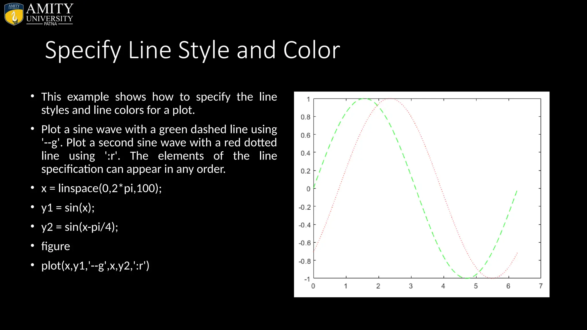
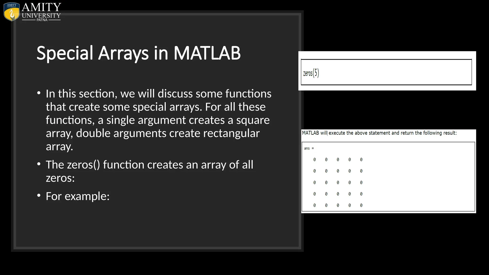
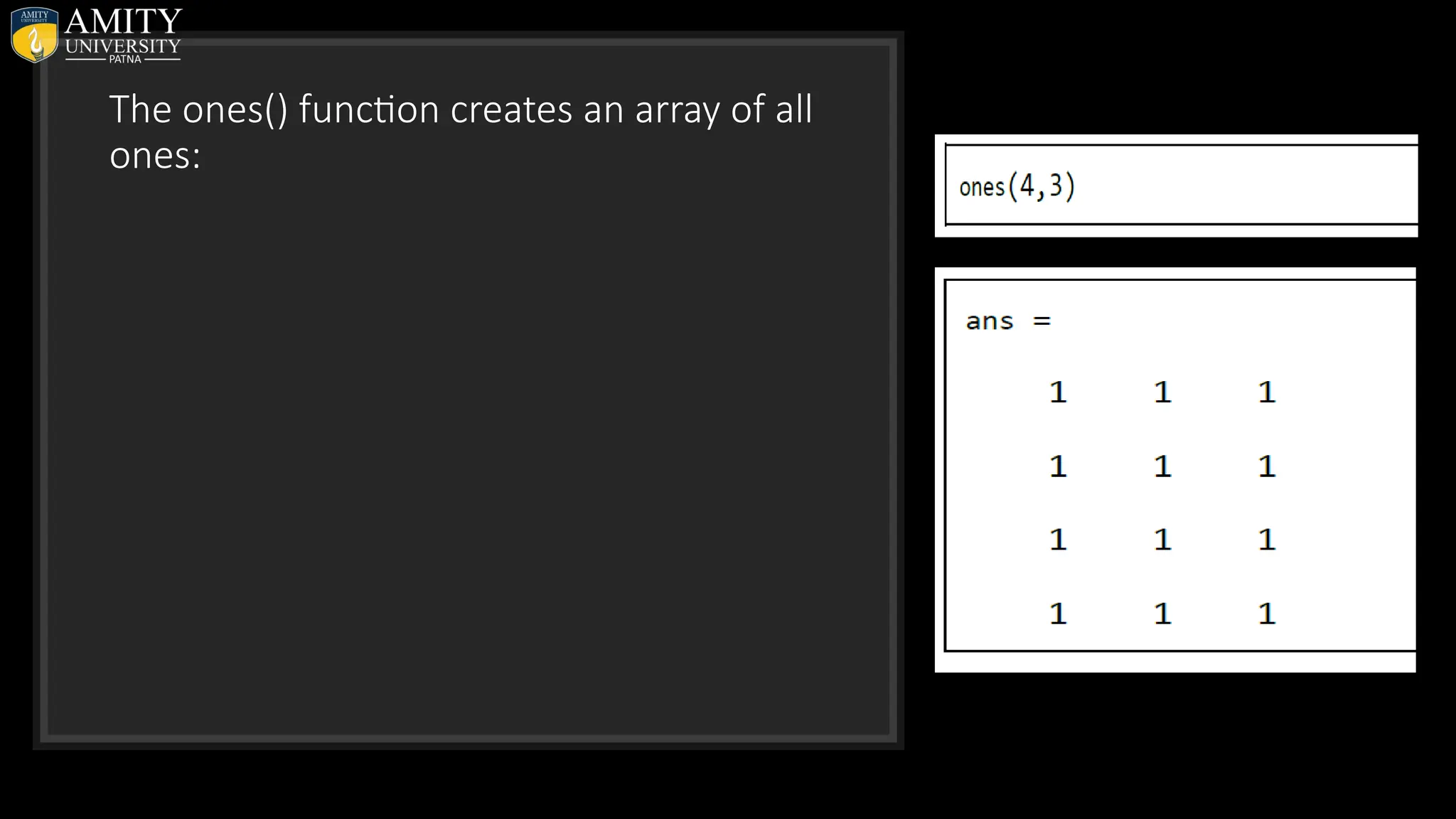
Download to read offline


![Commonly used Operators and Special Characters (Cont.) Operator Purpose . Array left-division operator. ./ Array right-division operator. : Colon; generates regularly spaced elements and represents an entire row or column. ( ) Parentheses; encloses function arguments and array indices; overrides precedence. [ ] Brackets; enclosures array elements. . Decimal point. … Ellipsis; line-continuation operator , Comma; separates statements and elements in a row ; Semicolon; separates columns and suppresses display. % Percent sign; designates a comment and specifies formatting. = Assignment operator.](https://image.slidesharecdn.com/matlab-250703055339-75318ae5/75/MATLAB-Introduction-Features-Display-Windows-Syntax-Operators-Graph-Plot-17-2048.jpg)
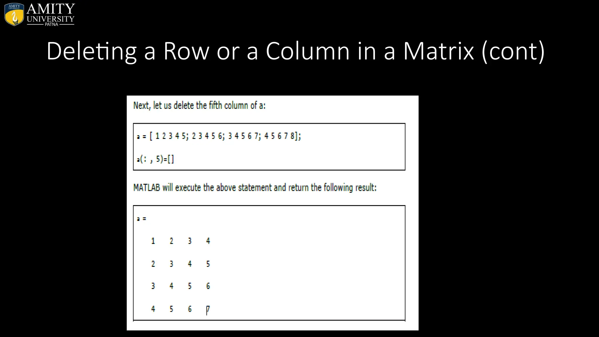
![Deleting a Row or a Column in a Matrix • You can delete an entire row or column of a matrix by assigning an empty set of square braces [] to that row or column. Basically, [] denotes an empty array. • For example, let us delete the fourth row of a: a = [ 1 2 3 4 5; 2 3 4 5 6; 3 4 5 6 7; 4 5 6 7 8]; a( 4 , : ) = [] MATLAB will execute the above statement and return the following result: a = 1 2 3 4 5 2 3 4 5 6 3 4 5 6 7](https://image.slidesharecdn.com/matlab-250703055339-75318ae5/75/MATLAB-Introduction-Features-Display-Windows-Syntax-Operators-Graph-Plot-26-2048.jpg)
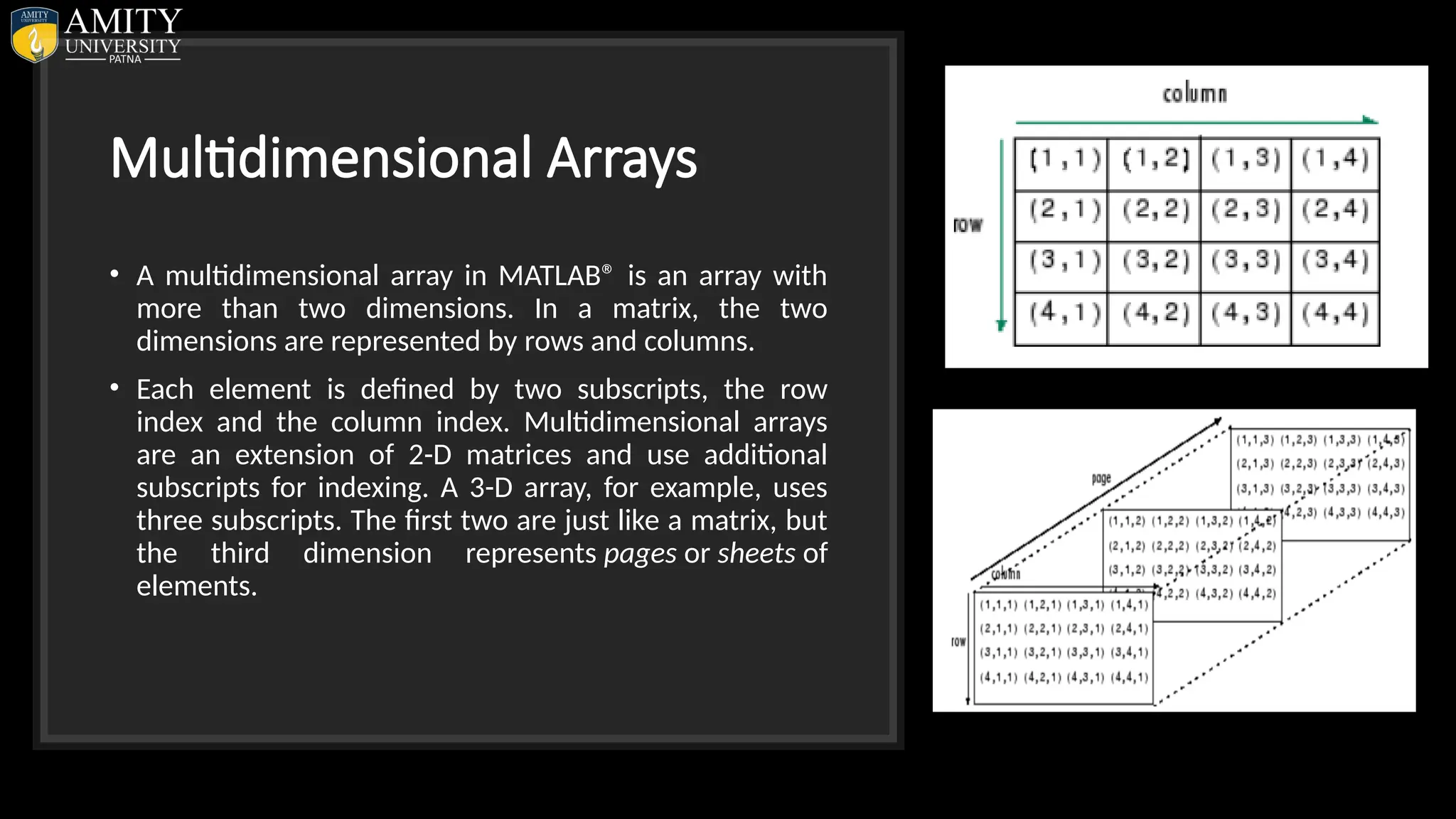
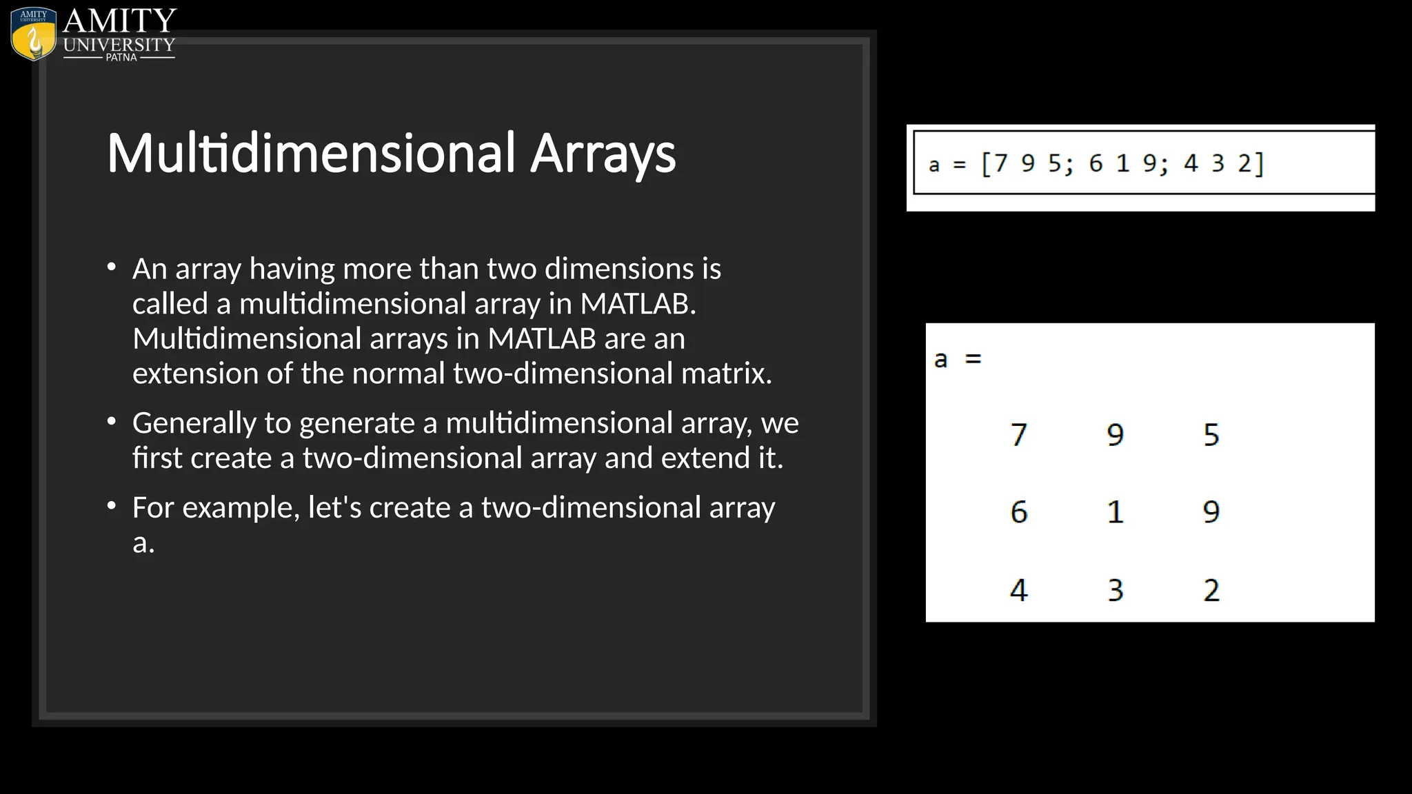
![ARRAYS • Arrays are Set of Elements having same data type or we can Say that Arrays are Collection of Elements having same name and same data type. • All variables of all data types in MATLAB are multidimensional arrays. • A vector is a one-dimensional array and a matrix is a two-dimensional array. • Two Dimensional Array or the Matrix • The Two Dimensional array is used for representing the elements of the array in the form of the rows and columns and these are used for representing the Matrix A Two Dimensional Array uses the two subscripts for declaring the elements of the Array • “Like this int a[3][3]” • This is the Example of the Two Dimensional Array In this first 3 represents the total number of Rows and the Second Elements Represents the Total number of Columns The Total Number of elements are judge by Multiplying the Numbers of Rows * Number of Columns. In the above array the Total Number of elements](https://image.slidesharecdn.com/matlab-250703055339-75318ae5/75/MATLAB-Introduction-Features-Display-Windows-Syntax-Operators-Graph-Plot-43-2048.jpg)
![We can also use the cat() function to build multidimensional arrays. It concatenates a list of arrays along a specified dimension: Syntax for the cat() function is: B = cat(3,A,[3 2 1; 0 9 8; 5 3 7])](https://image.slidesharecdn.com/matlab-250703055339-75318ae5/75/MATLAB-Introduction-Features-Display-Windows-Syntax-Operators-Graph-Plot-48-2048.jpg)
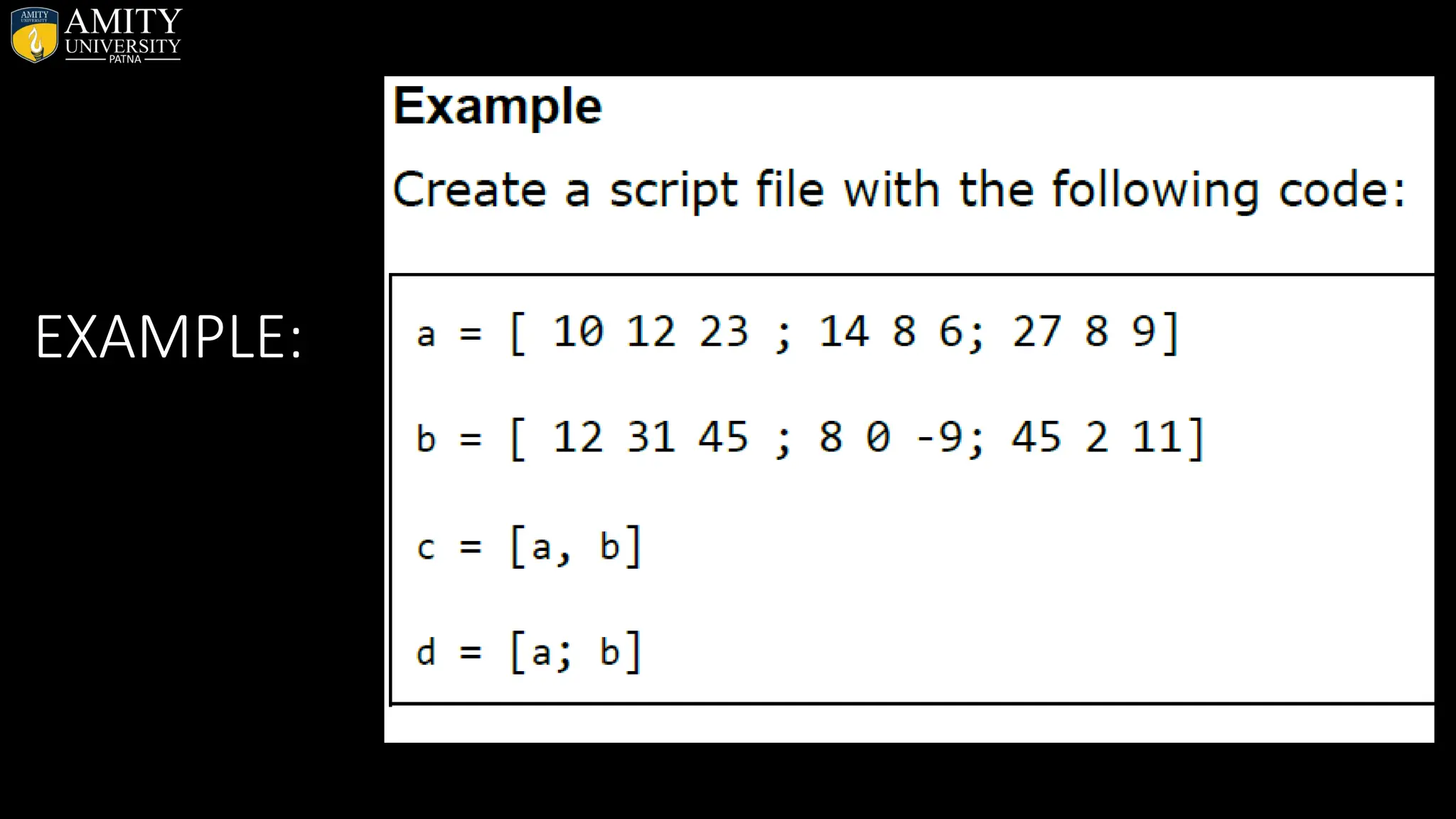
![Concatenating Matrice • You can concatenate two matrices to create a larger matrix. The pair of square brackets '[]' is the concatenation operator. • MATLAB allows two types of concatenations: • Horizontal concatenation • Vertical concatenation • When you concatenate two matrices by separating those using commas, they are just appended horizontally. It is called horizontal concatenation. • Alternatively, if you concatenate two matrices by separating those using semicolons, they are appended vertically. It is called vertical concatenation.](https://image.slidesharecdn.com/matlab-250703055339-75318ae5/75/MATLAB-Introduction-Features-Display-Windows-Syntax-Operators-Graph-Plot-51-2048.jpg)
![Reshape • Reshape array collapse all in page • Syntax • B = reshape(A,sz) • B = reshape(A,sz1,...,szN) EXAMPLE • h=[2 3 4 5;8 1 2 0;6 9 3 7] • g=reshape(h,6,2)](https://image.slidesharecdn.com/matlab-250703055339-75318ae5/75/MATLAB-Introduction-Features-Display-Windows-Syntax-Operators-Graph-Plot-56-2048.jpg)
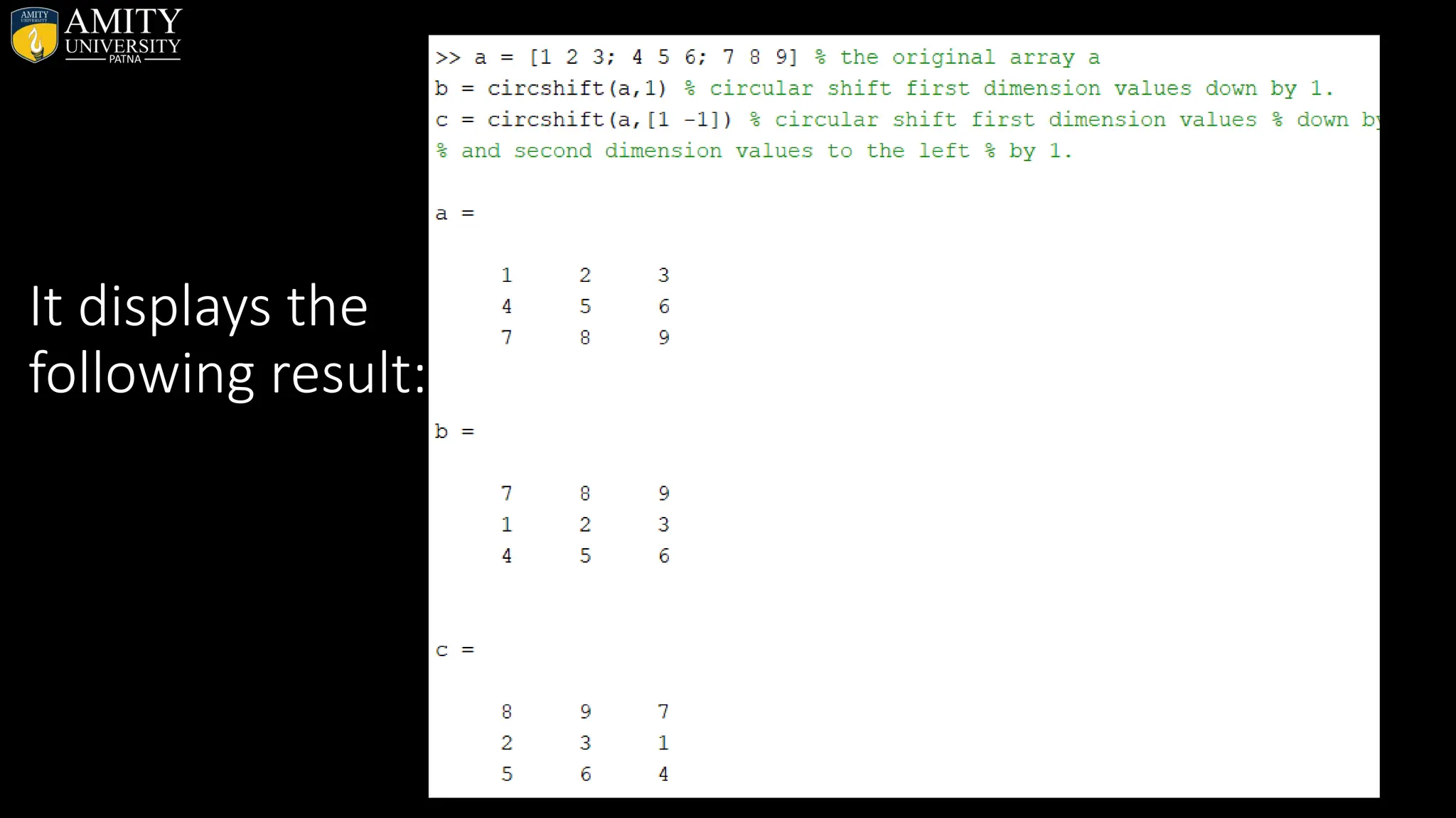
![Shifting the Matrix • Circular Shifting of the Array Elements: • Create a script file and type the following code into it: • a = [1 2 3; 4 5 6; 7 8 9] % the original array a • b = circshift(a,1) % circular shift first dimension values down by 1. • c = circshift(a,[1 -1]) % circular shift first dimension values % down by 1 • % and second dimension values to the left % by 1.](https://image.slidesharecdn.com/matlab-250703055339-75318ae5/75/MATLAB-Introduction-Features-Display-Windows-Syntax-Operators-Graph-Plot-59-2048.jpg)
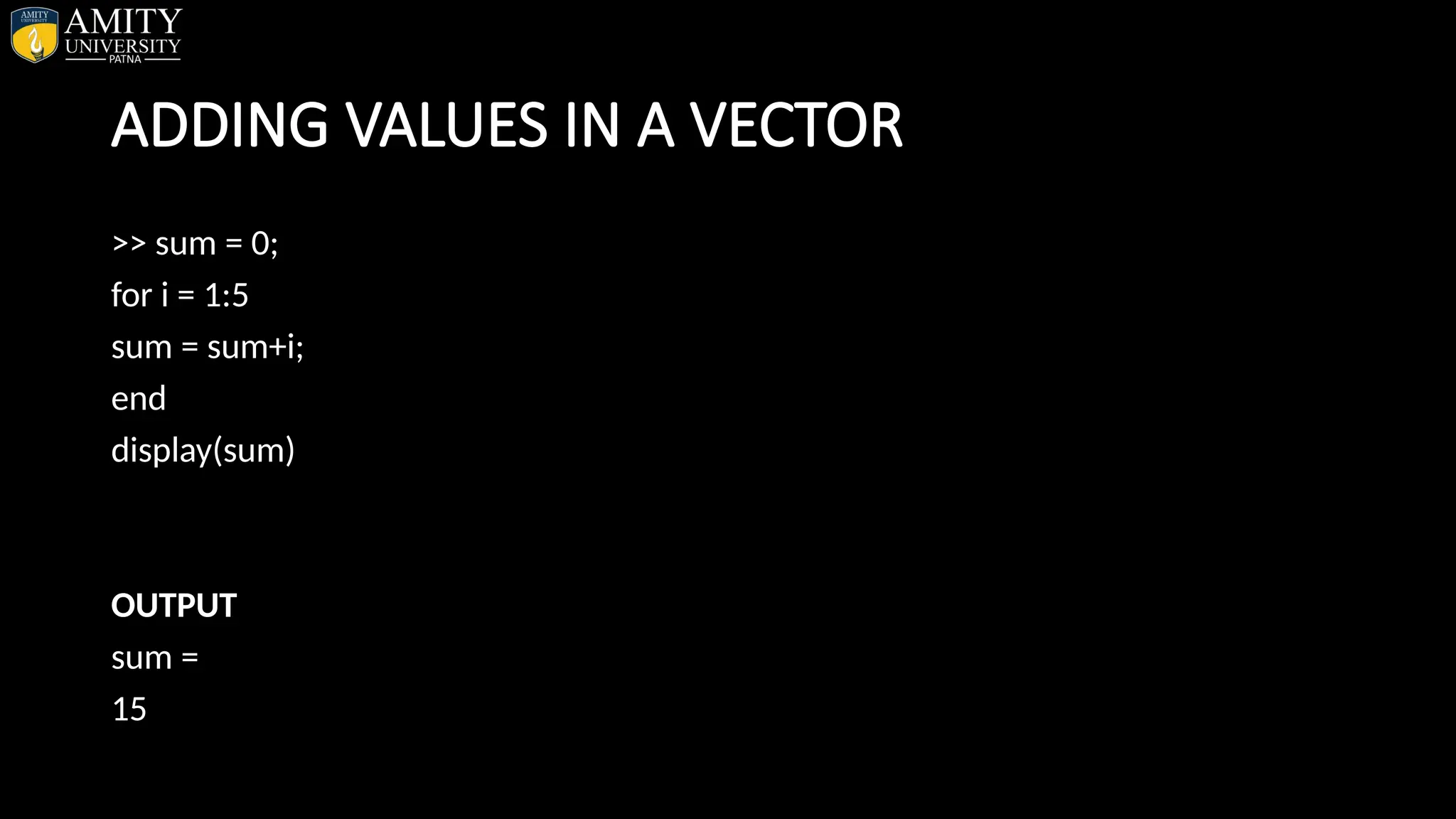
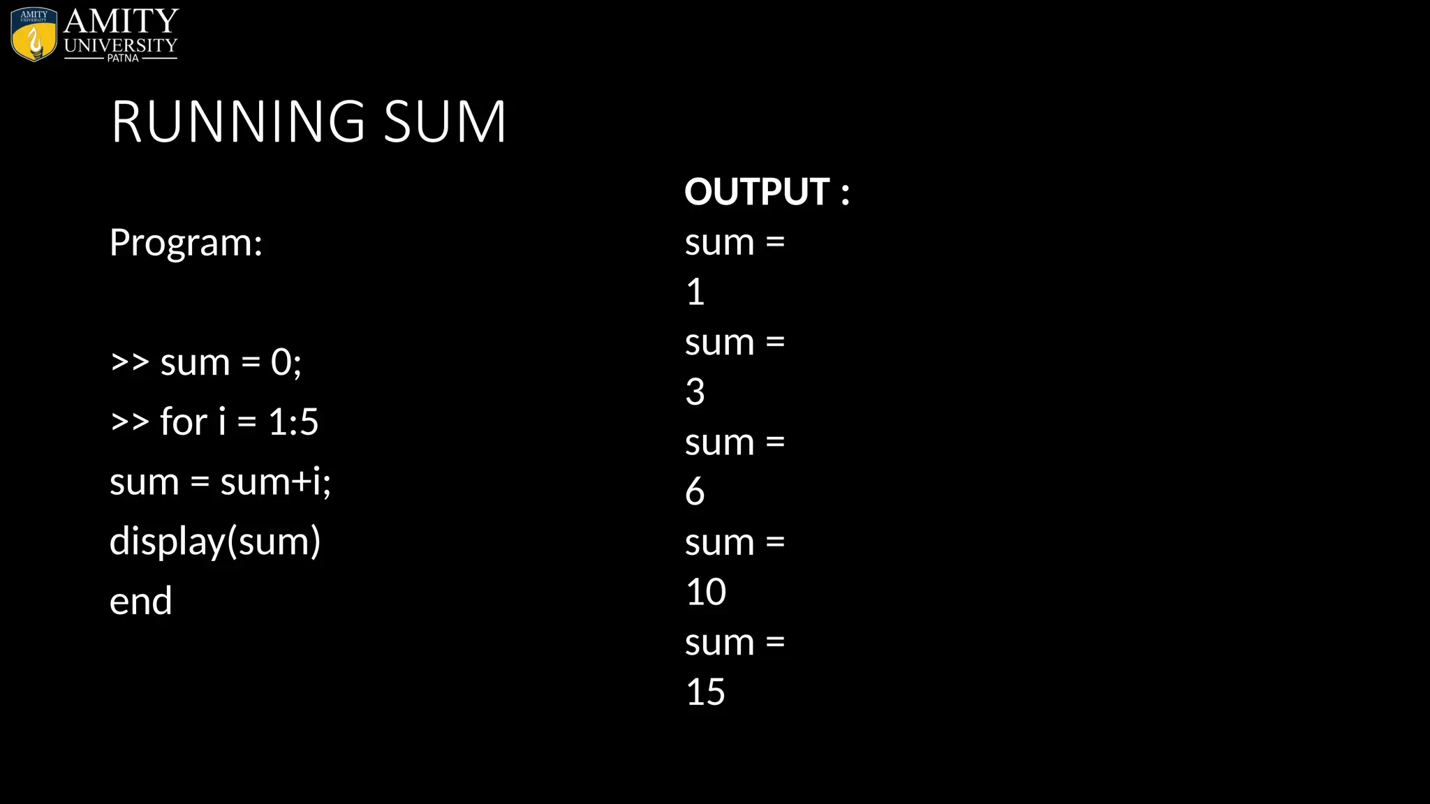
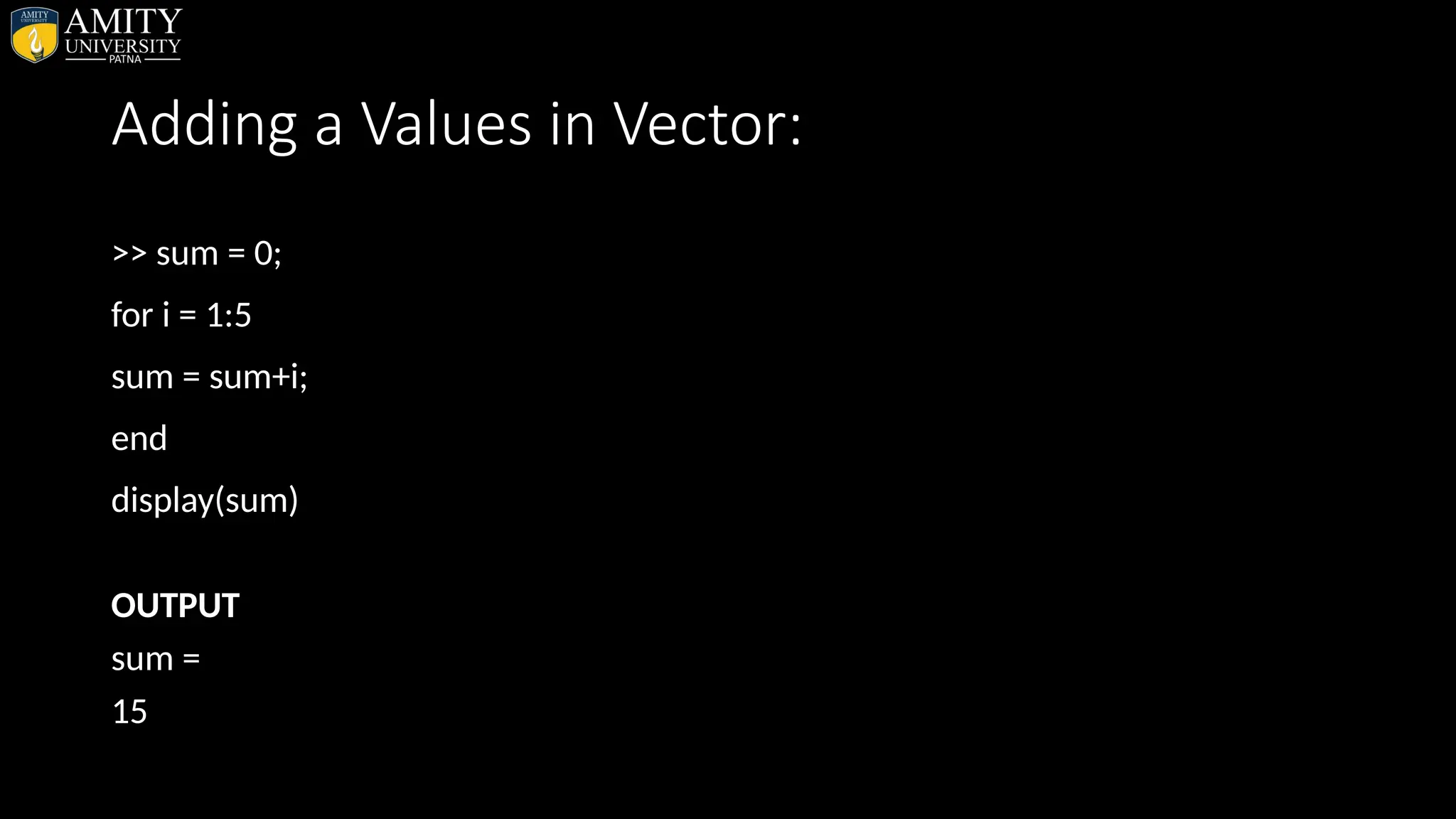
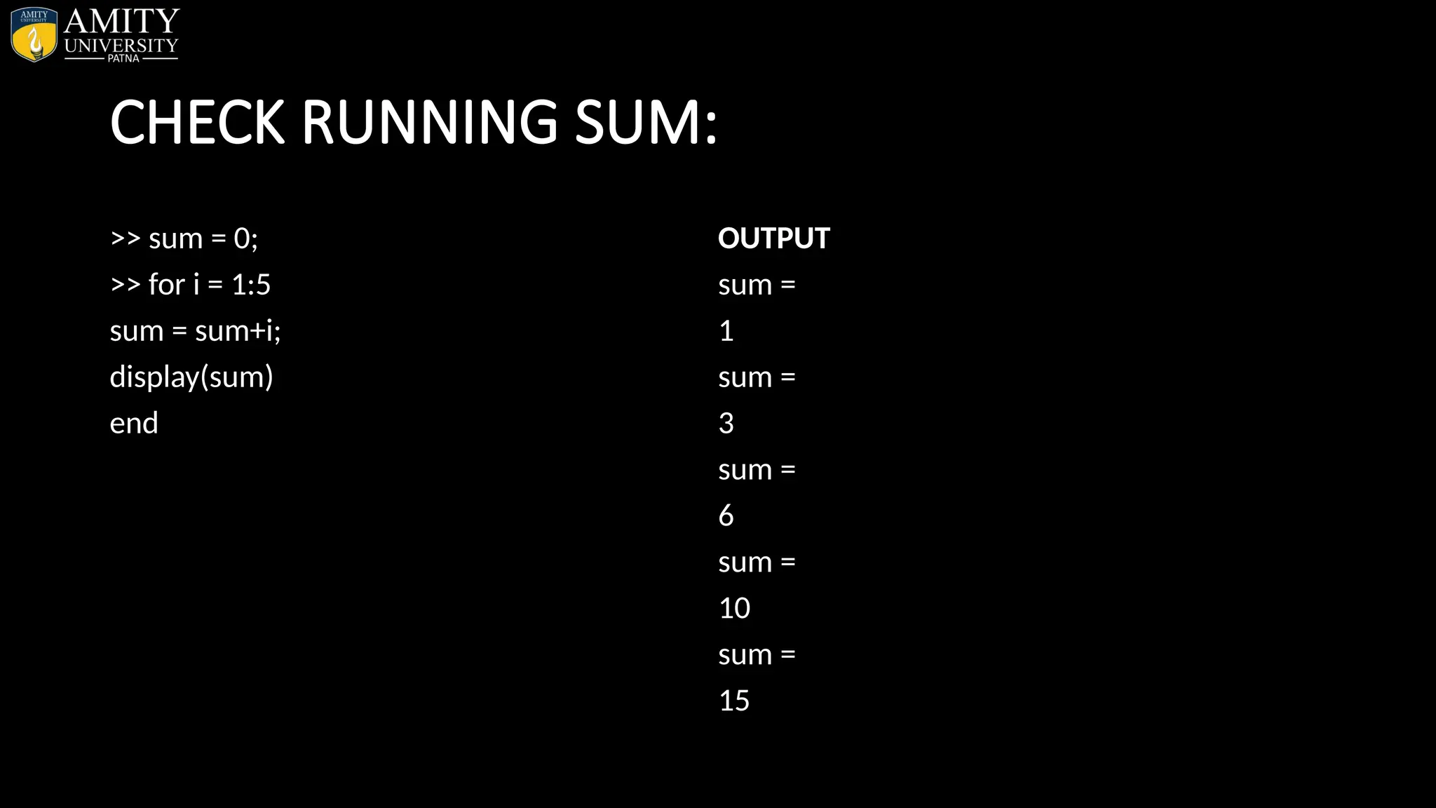
![CHECKING THE SUM CHECK SUM: >> A = [1 2 3 4 5] OUTPUT A = 1 2 3 4 5 >> B = sum(A) OUTPUT B = 15](https://image.slidesharecdn.com/matlab-250703055339-75318ae5/75/MATLAB-Introduction-Features-Display-Windows-Syntax-Operators-Graph-Plot-69-2048.jpg)
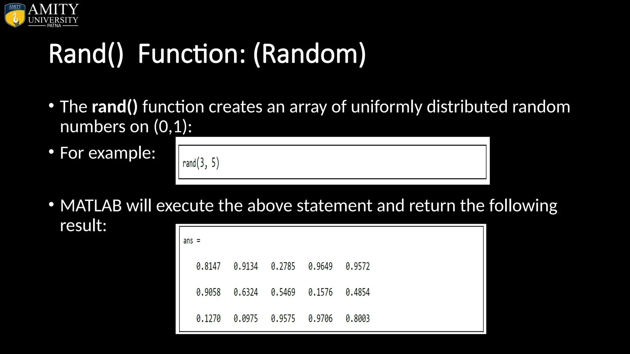
![Cumulative sum • Syntax –CUMSUM • Find the cumulative sum of the integers from 1 to 5. The element B(2) is the sum of A(1) and A(2), while B(5) is the sum of elements A(1) through A(5). Eg: >> A = [1 2 3 4 5] A = 1 2 3 4 5 >> B = cumsum(A) B = 1 3 6 10 15](https://image.slidesharecdn.com/matlab-250703055339-75318ae5/75/MATLAB-Introduction-Features-Display-Windows-Syntax-Operators-Graph-Plot-71-2048.jpg)
![CHECK SUM: • >> A = [1 2 3 4 5] OUTPUT A = 1 2 3 4 5 >> B = sum(A) OUTPUT B = 15](https://image.slidesharecdn.com/matlab-250703055339-75318ae5/75/MATLAB-Introduction-Features-Display-Windows-Syntax-Operators-Graph-Plot-74-2048.jpg)
![CHECK CUMSUM: • >> A = [1 2 3 4 5] OUTPUT A = 1 2 3 4 5 >> B = cumsum(A) OUTPUT B = 1 3 6 10 15](https://image.slidesharecdn.com/matlab-250703055339-75318ae5/75/MATLAB-Introduction-Features-Display-Windows-Syntax-Operators-Graph-Plot-76-2048.jpg)
![Examples with syntax (Rounding Functions) • 1. ROUND >>round(3.67) • OUTPUT ans = 4 • 2. FLOOR >>floor(3.67) • OUTPUT ans = 3 • 3. CEIL >>ceil(3.67) • OUTPUT ans = 4 • 4. FIX >>a = [1.88 2.05 9.54 8.5] • OUTPUT • a = 1.8800 2.0500 9.5400 8.5000 >>fix(a) • ans = 1 2 9 8](https://image.slidesharecdn.com/matlab-250703055339-75318ae5/75/MATLAB-Introduction-Features-Display-Windows-Syntax-Operators-Graph-Plot-80-2048.jpg)

![• Sphere Plot • The sphere function generates the x-, y-, and z-coordinates of a unit sphere for use with surf and mesh. • sphere generates a sphere consisting of 20-by-20 faces. • sphere(n) draws a surf plot of an n-by-n sphere in the current figure. • [X,Y,Z] = sphere(n) returns the coordinates of a sphere in three matrices that are (n+1)-by-(n+1) in size. You draw the sphere with surf(X,Y,Z) or mesh(X,Y,Z).](https://image.slidesharecdn.com/matlab-250703055339-75318ae5/75/MATLAB-Introduction-Features-Display-Windows-Syntax-Operators-Graph-Plot-110-2048.jpg)
![• Cylinder Plot • cylinder generates x-, y-, and z-coordinates of a unit cylinder. You can draw the cylindrical object using surf ormesh, or draw it immediately by not providing output arguments. • [X,Y,Z] = cylinder returns the x-, y-, and z-coordinates of a cylinder with a radius equal to 1. The cylinder has 20 equally spaced points around its circumference.](https://image.slidesharecdn.com/matlab-250703055339-75318ae5/75/MATLAB-Introduction-Features-Display-Windows-Syntax-Operators-Graph-Plot-113-2048.jpg)
![3-D Contour Lines • >>x = -2:0.25:2; • >>[X,Y] = meshgrid(x); • >>Z = X.*exp(-X.^2-Y.^2); • >>contour3(X,Y,Z,30) • Output:](https://image.slidesharecdn.com/matlab-250703055339-75318ae5/75/MATLAB-Introduction-Features-Display-Windows-Syntax-Operators-Graph-Plot-115-2048.jpg)
![Pie Chart & Bar Chart • >> x = [1,2,3,4,5,6,7,8]; • >> pie(x); • Output: • >> z = magic(5); • >> b = bar3(z); • Output:](https://image.slidesharecdn.com/matlab-250703055339-75318ae5/75/MATLAB-Introduction-Features-Display-Windows-Syntax-Operators-Graph-Plot-116-2048.jpg)

Introduction to MATLAB MATLAB (MATrix LABoratory) is a fourth-generation high-level programming language and interactive environment for numerical computation, visualization and programming. MATLAB is developed by MathWorks. It allows matrix manipulations; plotting of functions and data; implementation of algorithms; creation of user interfaces; interfacing with programs written in other languages, including C, C++, Java, and FORTRAN; analyze data; develop algorithms; and create models and applications. It has numerous built-in commands and math functions that help you in mathematical calculations, generating plots, and performing numerical methods. Uses of MATLAB MATLAB is widely used as a computational tool in science and engineering encompassing the fields of physics, chemistry, math and all engineering streams. It is used in a range of applications including: Signal processing and Communications Image and video Processing Control systems Test and measurement Computational finance Computational biology Algorithm development Data acquisition Modeling, simulation, and prototyping Data analysis, exploration, and visualization Scientific and engineering graphics Application development, including graphical user interface building