Matlab Functions for programming fundamentals

Matlab Functions for programming fundamentals

• 1.
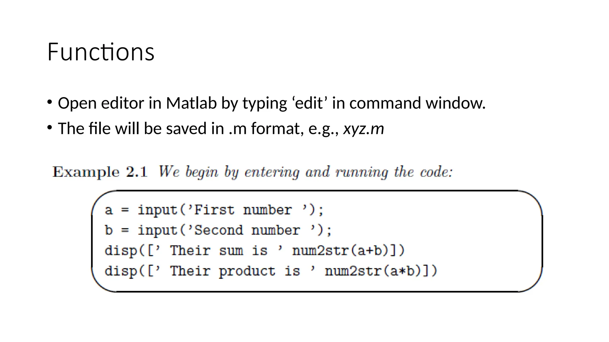
  Functions • Open editorin Matlab by typing ‘edit’ in command window. • The file will be saved in .m format, e.g., xyz.m
• 2.
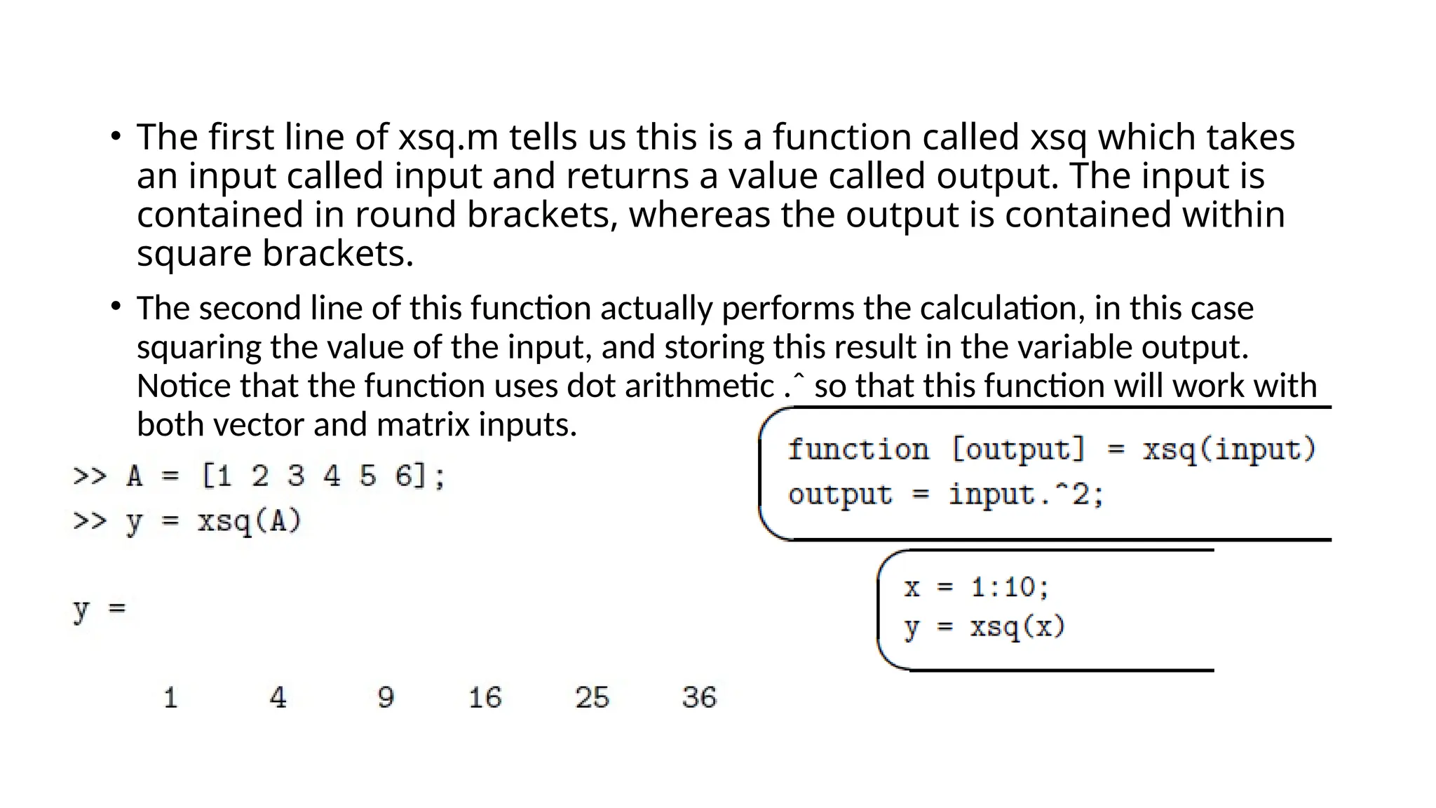
  • The firstline of xsq.m tells us this is a function called xsq which takes an input called input and returns a value called output. The input is contained in round brackets, whereas the output is contained within square brackets. • The second line of this function actually performs the calculation, in this case squaring the value of the input, and storing this result in the variable output. Notice that the function uses dot arithmetic .ˆ so that this function will work with both vector and matrix inputs.
• 3.
  Example 2.3: Supposewe want to plot contours of a function of two variables z = x2 + y2 . We can use the code. function [output] = func (x,y) output = x.ˆ2 + y.ˆ2; x = 0.0:pi/10:pi; y = x; [X,Y] = meshgrid(x,y); f = func(X,Y); contour(X,Y,f) axis([0 pi 0 pi]) axis equal
• 4.
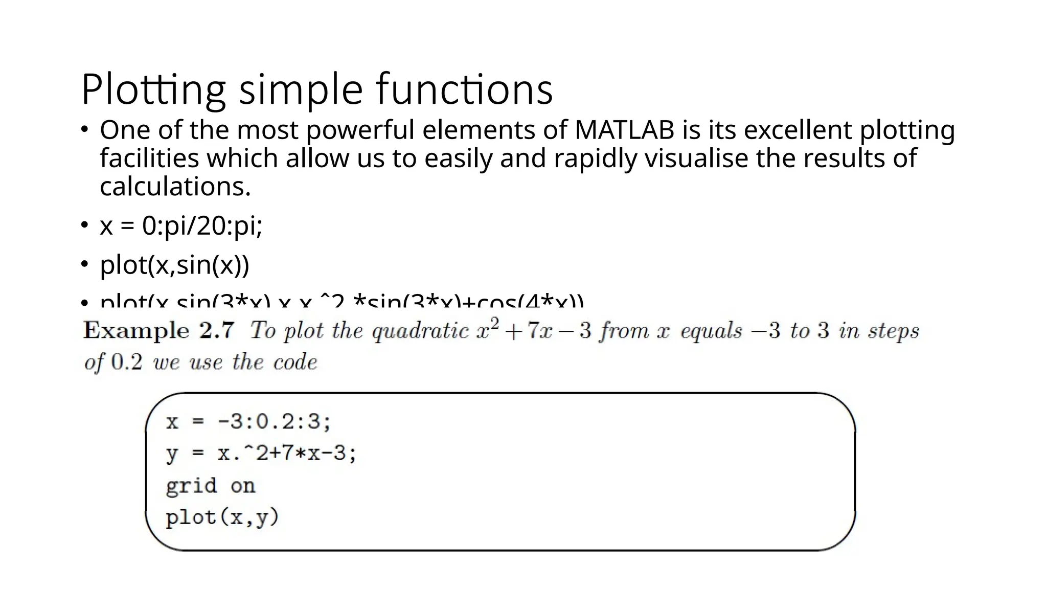
  Plotting simple functions •One of the most powerful elements of MATLAB is its excellent plotting facilities which allow us to easily and rapidly visualise the results of calculations. • x = 0:pi/20:pi; • plot(x,sin(x)) • plot(x,sin(3*x),x,x.ˆ2.*sin(3*x)+cos(4*x))
• 5.
  Example 2.8 x =0:pi/20:pi; n = length(x); r = 1:n/7:n; y = x.ˆ2+3; plot(x,y,’b’,x(r),y(r),’r*’) axis([-pi/3 pi+pi/3 -1 15]) xlabel(’x values’) ylabel(’Function values’) title(’Demonstration plot’) text(pi/10,0,’alpha=betaˆ2’)
• 6.
  3D Graphs • Oneof the excellent features of MATLAB is the way in which it handles two and three-dimensional graphics. Although we will have little need to exploit the power of MATLAB’s graphical rendering we should be aware of the basic commands. Examples serve to highlight some of the many possibilities: x = linspace(-pi/2,pi/2,40); y = x; [X,Y] = meshgrid(x,y); f = sin(X.ˆ2-Y.ˆ2); figure(1) contour(X,Y,f) figure(2) contourf(X,Y,f,20) figure(3) surf(X,Y,f)
• 7.
  Derivative of afunction % % evaluate_poly2.m % function [f, fprime] = evaluate_poly2(x) f = 3*x.ˆ2+2*x+1; fprime = 6*x+2; • This MATLAB function calculates the values of the polynomial and its derivative. This could be called using the sequence of commands x = -5:0.5:5; [func,dfunc] = evaluate_poly2(x);
• 8.
  Evaluating Polynomials andPlotting Curves % quadratic.m % This program evaluates a quadratic % at a certain value of x % The coefficients are stored in a2, a1 and a0. % SRO & JPD % str = ’Please enter the ’; a2 = input([str ’coefficient of x squared: ’]); a1 = input([str ’coefficient of x: ’]); a0 = input([str ’constant term: ’]); x = input([str ’value of x: ’]); y = a2*x*x+a1*x+a0; % Now display the result disp([’Polynomial value is: ’ num2str(y)])
• 9.
  % % evaluate_poly.m % function [value]= evaluate_poly(x) value = 3*x.ˆ2+2*x+1;
• 10.
  Advantages of functions •Functions allow you to break down large, complex problems to smaller, more manageable pieces. • Functional decomposition. • Code reuse • Generality • A function can solve a set of related problems, not just a specific one by accepting input arguments. • For example, the built in function plot can draw a wide range of figures based on its input.
• 11.
  Errors – NumericalErrors • It is very hard to get computers to perform exact calculations. • If we add (or subtract) integers then a computer can be expected to get the exact answer, but even this operation has its limits. • Once we try to perform the division operation we run into trouble. • Almost all numerical schemes are prone to some kind of error. It is important to bear this in mind and understand the possible extent of the error. Errors can be expressed as two basic types: • Absolute error: This is the difference between the exact answer and the numerical answer. • Relative error: This is the absolute error divided by the size of the answer (either the numerical one or the exact one), which is often converted to a percentage.
• 12.
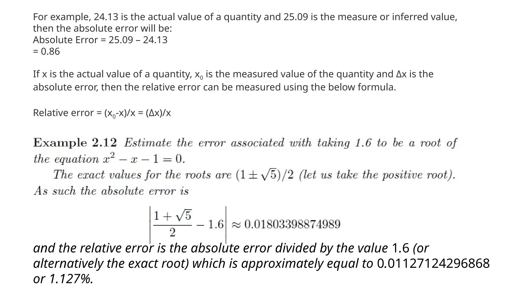
  and the relativeerror is the absolute error divided by the value 1.6 (or alternatively the exact root) which is approximately equal to 0.01127124296868 or 1.127%. For example, 24.13 is the actual value of a quantity and 25.09 is the measure or inferred value, then the absolute error will be: Absolute Error = 25.09 – 24.13 = 0.86 Relative error = (x0-x)/x = (Δx)/x If x is the actual value of a quantity, x0 is the measured value of the quantity and Δx is the absolute error, then the relative error can be measured using the below formula.
• 13.
  User Errors • Themost severe user errors will often cause MATLAB to generate error messages; these can help us to understand and identify where in our code we have made a mistake. • 1. Incorrect use of variable names. This may be due to a typographical error which has resulted in changes during the coding. • 2. Incorrect use of operators. The most common instance of this error occurs with dot arithmetic. • 3. Syntactical errors still produce feasible MATLAB code. For instance in order to evaluate the expression cos x, we should use cos(x): unfortunately the expression cos x also yields an answer (which is incorrect); somewhat bizarrely cos pi yields a row vector (which has the cosines of the ASCII values of the letters p and i as elements).
• 14.
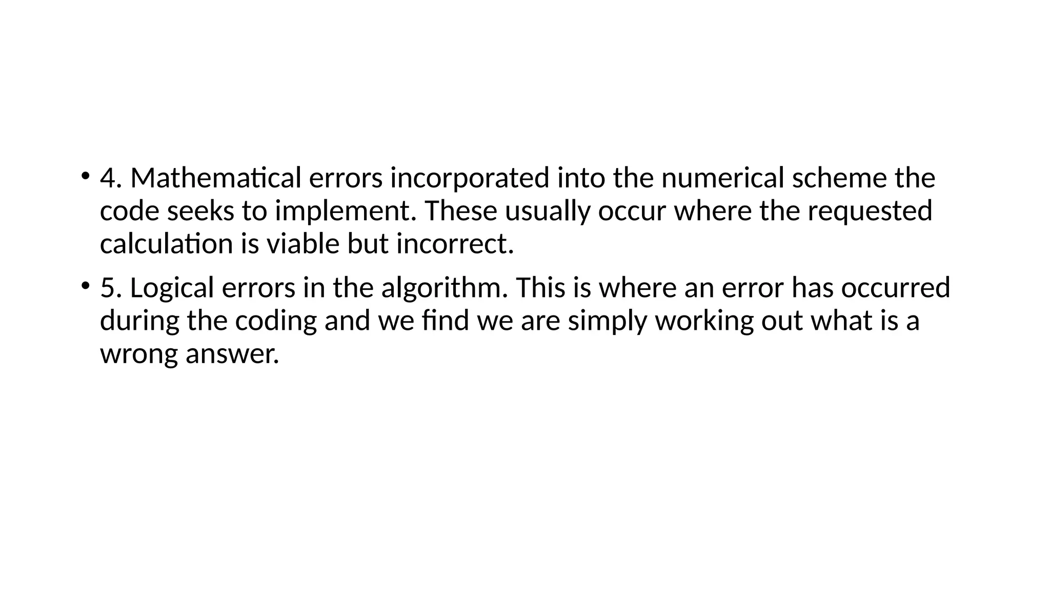
  • 4. Mathematicalerrors incorporated into the numerical scheme the code seeks to implement. These usually occur where the requested calculation is viable but incorrect. • 5. Logical errors in the algorithm. This is where an error has occurred during the coding and we find we are simply working out what is a wrong answer.
• 15.
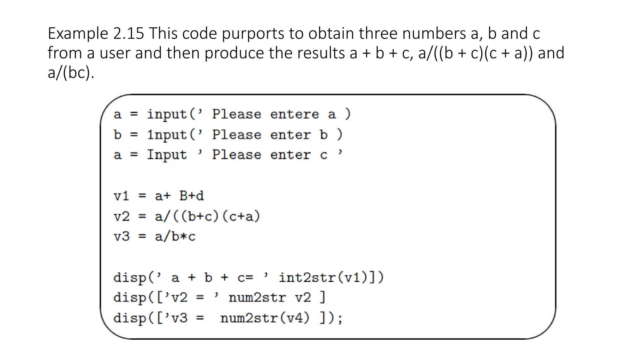
  Example 2.15 Thiscode purports to obtain three numbers a, b and c from a user and then produce the results a + b + c, a/((b + c)(c + a)) and a/(bc).