Download to read offline


![What is a data set? • Data Set • In the mind of a computer, a data set is any collection of data. It can be anything from an array to a complete database. • Example of an array: • [99,86,87,88,111,86,103,87,94,78,77,85,86]](https://image.slidesharecdn.com/mlteachtechtoe-200321044532/75/Machine-Learning-with-Python-made-easy-and-simple-3-2048.jpg)


![Machine Learning - Mean Median Mode In Machine Learning (and in mathematics) there are often three values that interests us: • Mean - The average value • Median - The mid point value • Mode - The most common value • Example: We have registered the speed of 13 cars: • speed = [99,86,87,88,111,86,103,87,94,78,77,85,86]](https://image.slidesharecdn.com/mlteachtechtoe-200321044532/75/Machine-Learning-with-Python-made-easy-and-simple-8-2048.jpg)
![Standard Deviation: • Standard deviation is a number that describes how spread out the values are. • A low standard deviation means that most of the numbers are close to the mean (average) value. • A high standard deviation means that the values are spread out over a wider range. • Example: This time we have registered the speed of 7 cars: • speed = [86,87,88,86,87,85,86] • The standard deviation is: • 0.9](https://image.slidesharecdn.com/mlteachtechtoe-200321044532/75/Machine-Learning-with-Python-made-easy-and-simple-9-2048.jpg)
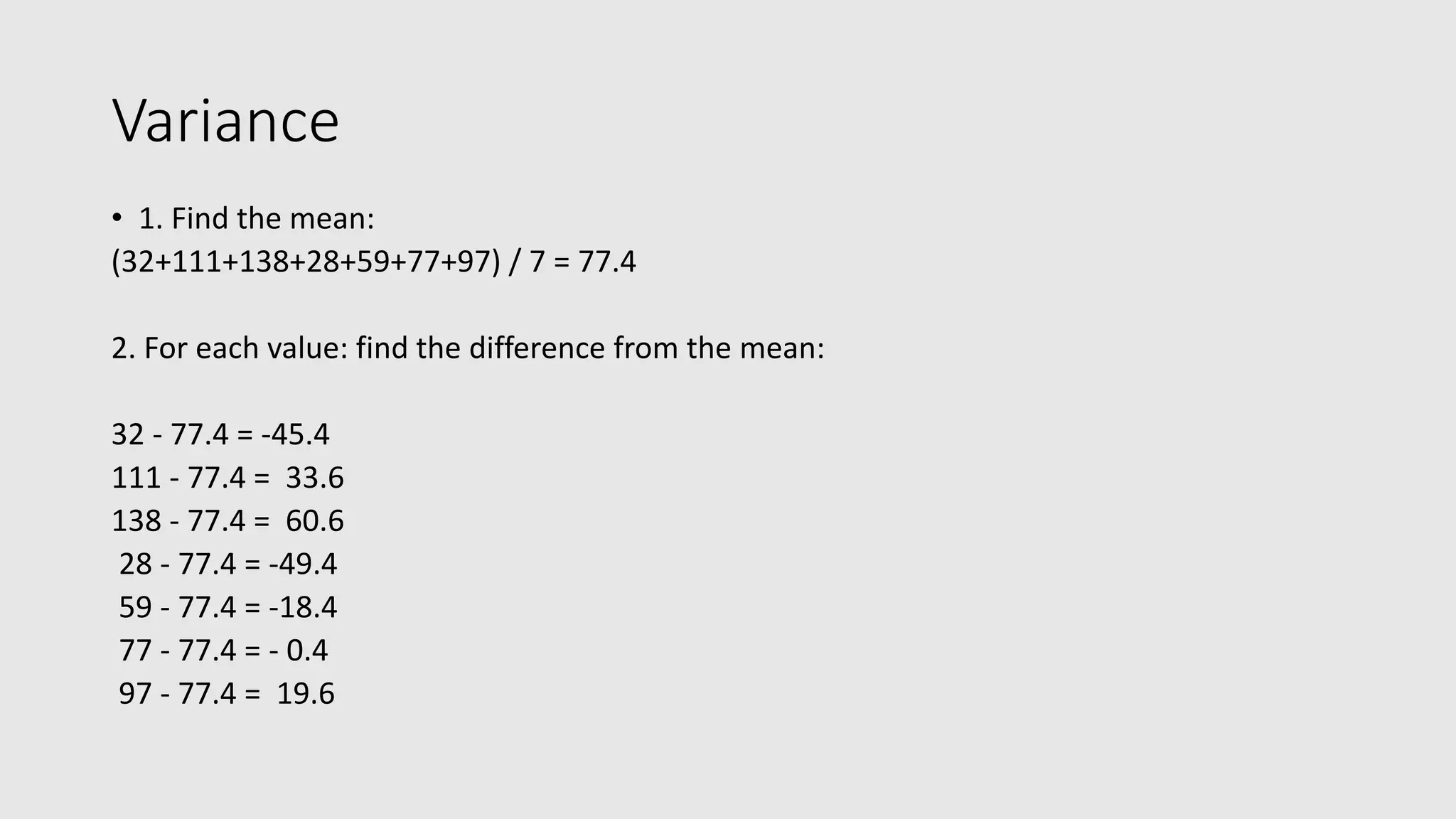
![Standard Deviation: • Meaning that most of the values are within the range of 0.9 from the mean value, which is 86.4. • Let us do the same with a selection of numbers with a wider range: • speed = [32,111,138,28,59,77,97] • The standard deviation is: 37.85 • Meaning that most of the values are within the range of 37.85 from the mean value, which is 77.4. • As you can see, a higher standard deviation indicates that the values are spread out over a wider range. • The NumPy module has a method to calculate the standard deviation:](https://image.slidesharecdn.com/mlteachtechtoe-200321044532/75/Machine-Learning-with-Python-made-easy-and-simple-10-2048.jpg)
![Machine Learning - Percentiles • What are Percentiles? • Percentiles are used in statistics to give you a number that describes the value that a given percent of the values are lower than. • Example: Let's say we have an array of the ages of all the people that lives in a street. • ages = [5,31,43,48,50,41,7,11,15,39,80,82,32,2,8,6,25,36,27,61,31] • What is the 75. percentile? The answer is 43, meaning that 75% of the people are 43 or younger.](https://image.slidesharecdn.com/mlteachtechtoe-200321044532/75/Machine-Learning-with-Python-made-easy-and-simple-16-2048.jpg)
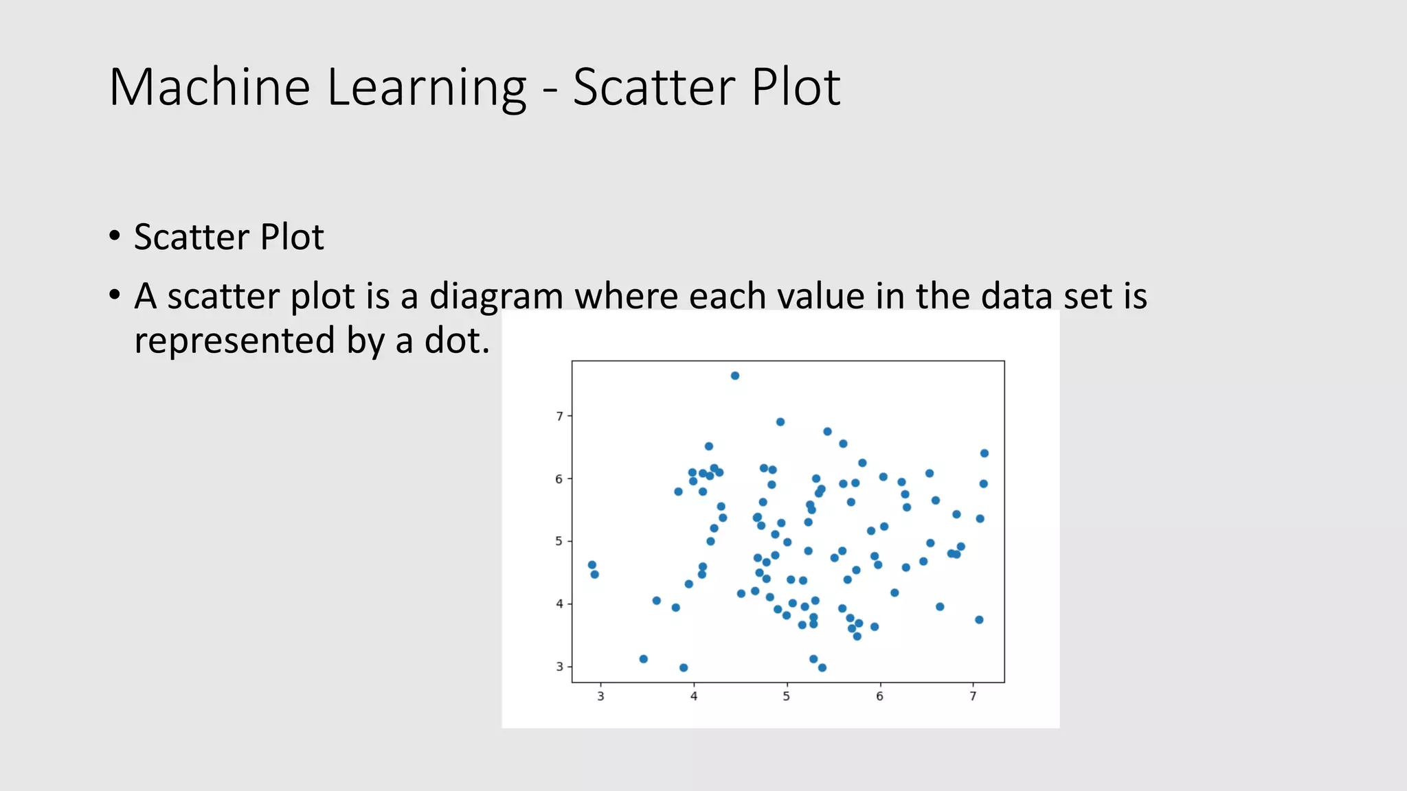
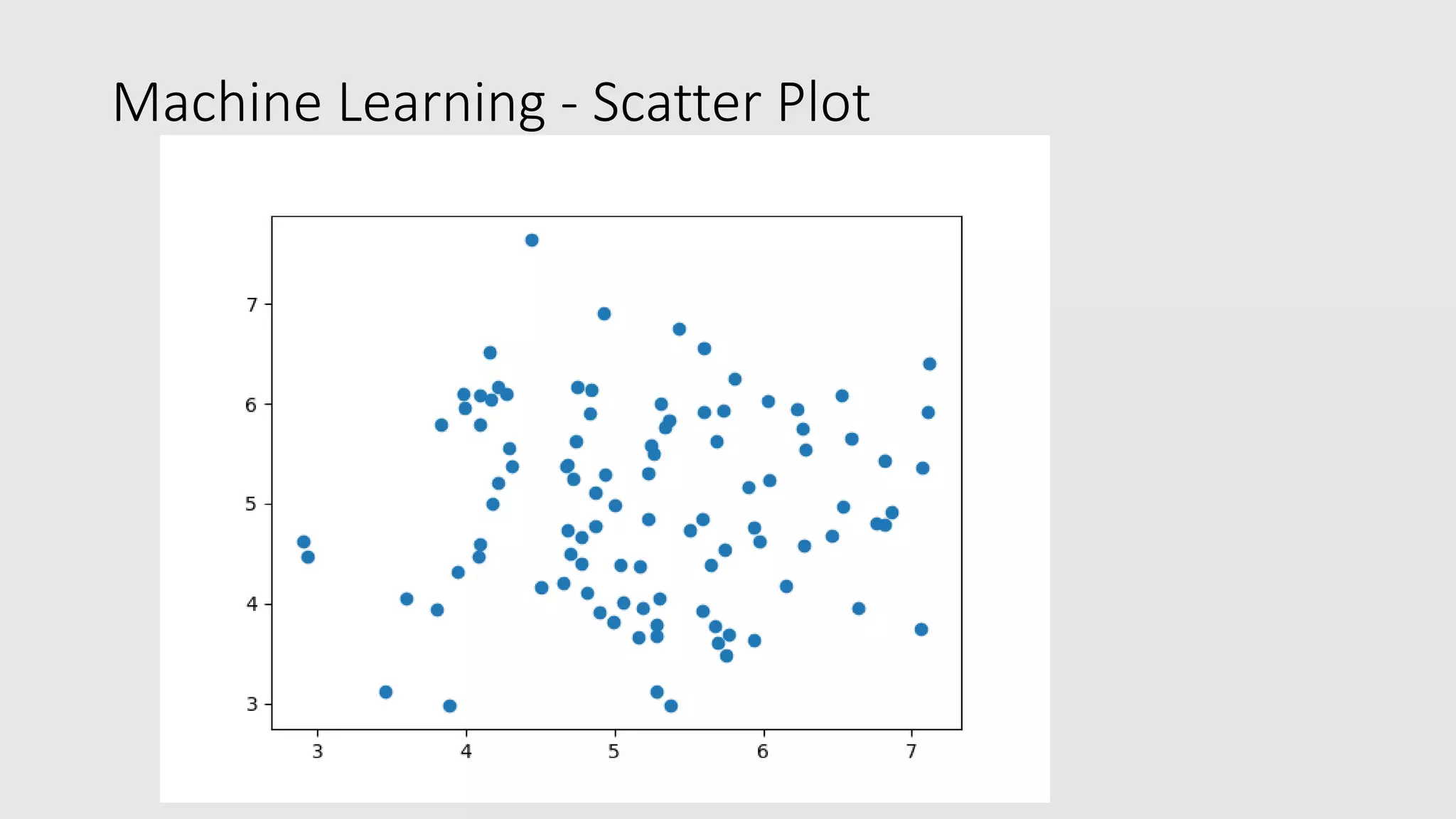
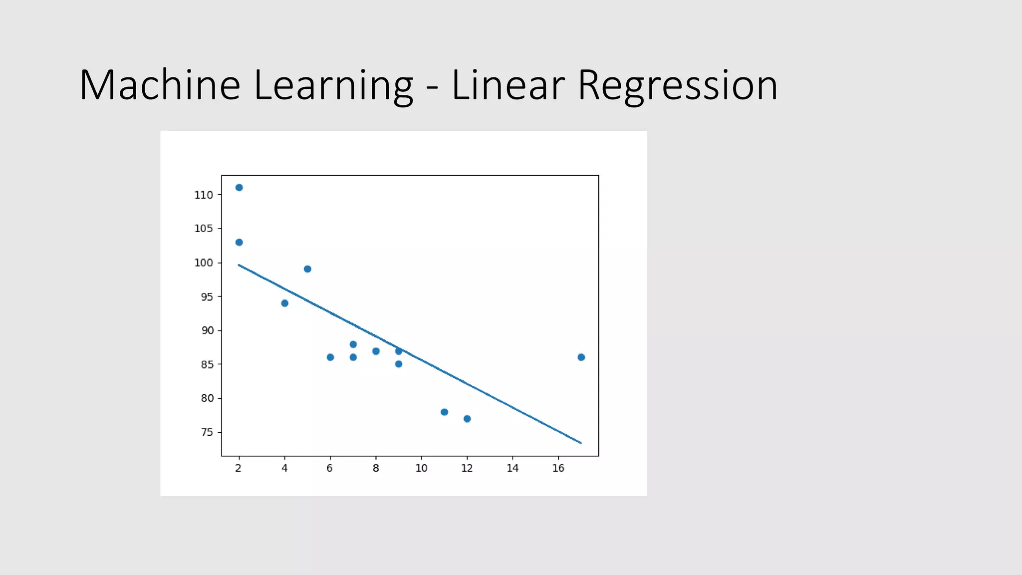
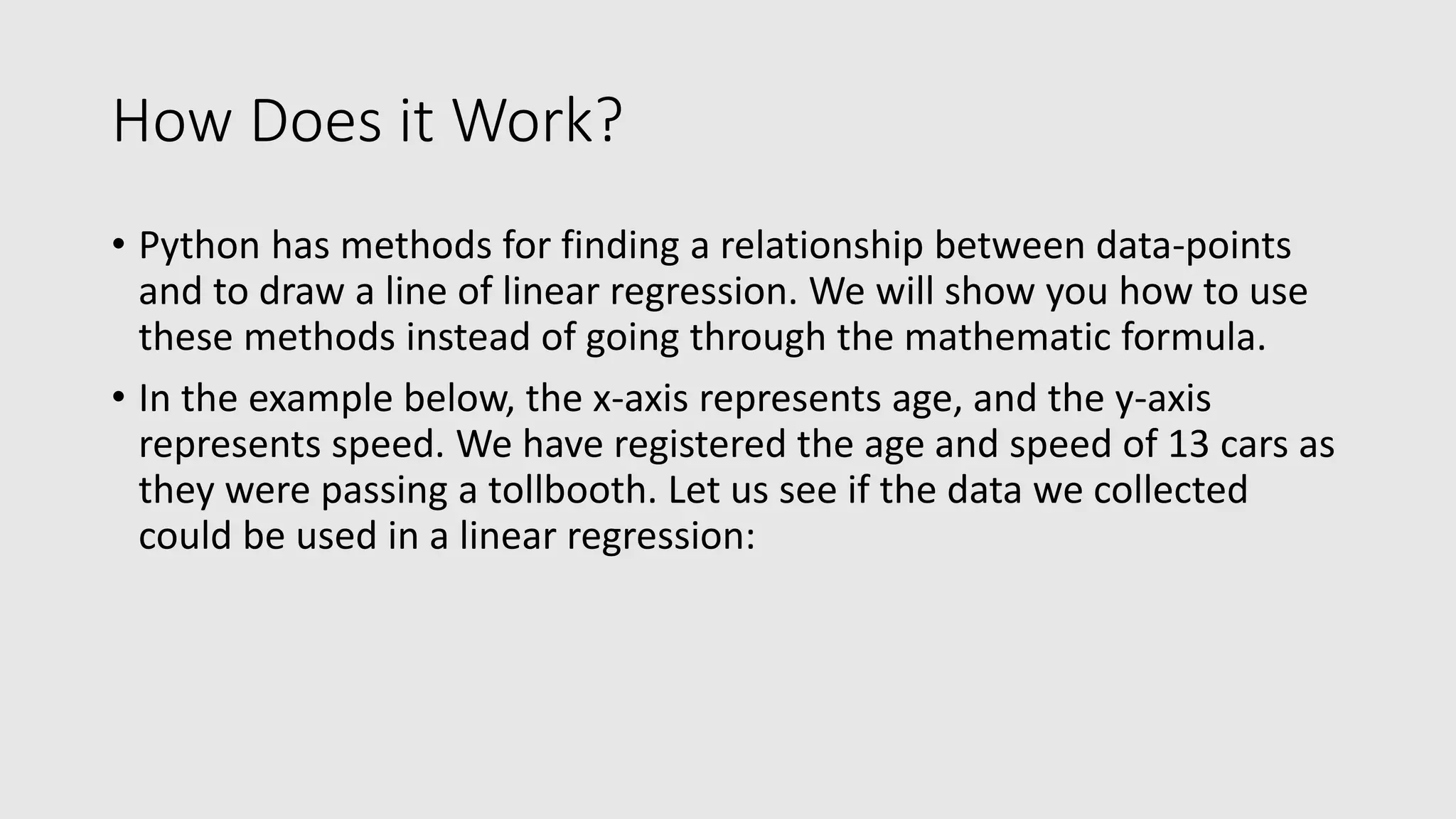
![Machine Learning - Scatter Plot • The Matplotlib module has a method for drawing scatter plots, it needs two arrays of the same length, one for the values of the x-axis, and one for the values of the y-axis: • x = [5,7,8,7,2,17,2,9,4,11,12,9,6] • y = [99,86,87,88,111,86,103,87,94,78,77,85,86] • The x array represents the age of each car. • The y array represents the speed of each car.](https://image.slidesharecdn.com/mlteachtechtoe-200321044532/75/Machine-Learning-with-Python-made-easy-and-simple-21-2048.jpg)


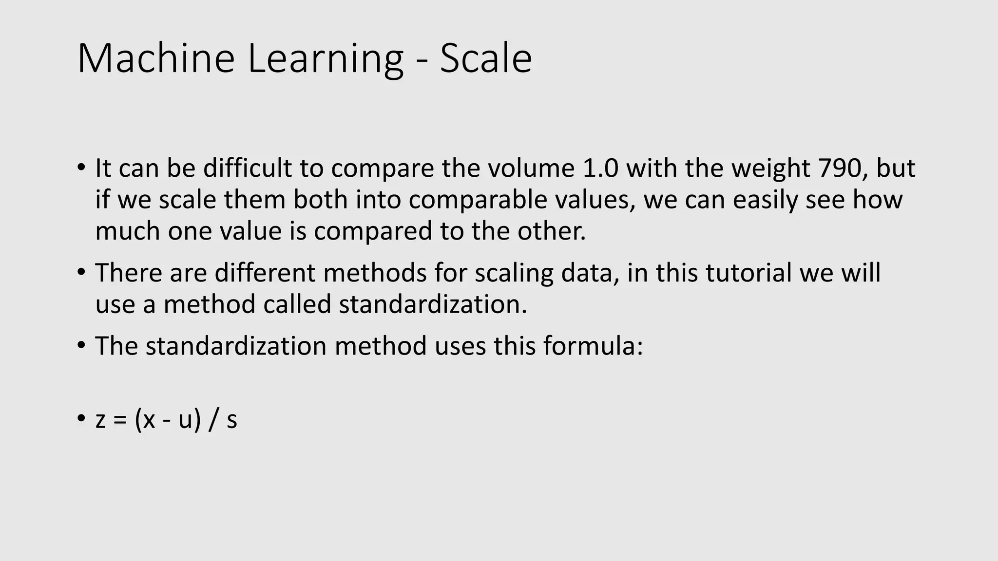
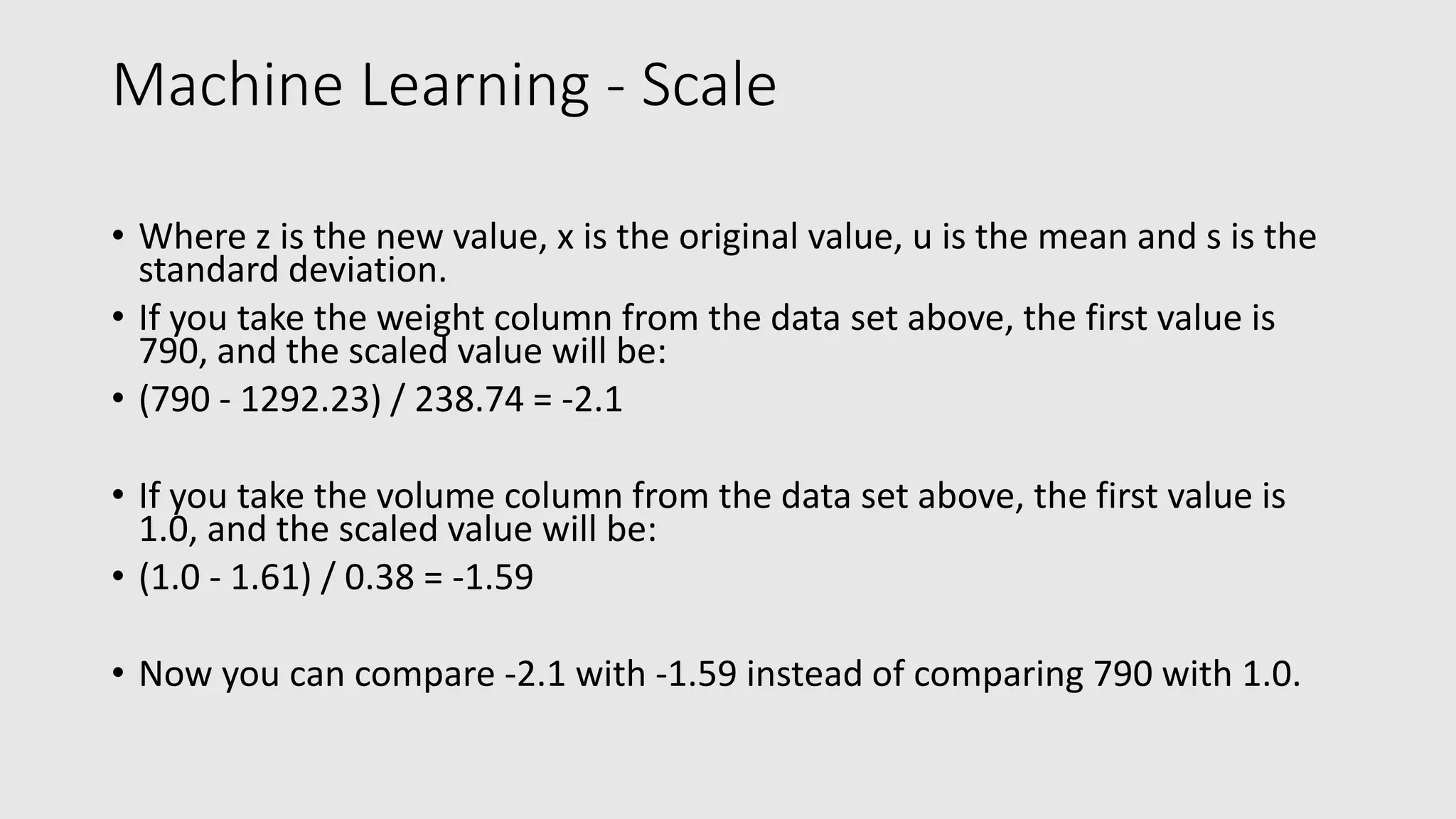


The document provides an overview of machine learning using Python, explaining key concepts such as the definition of machine learning, data sets, types of data, and various statistical measures like mean, median, mode, and standard deviation. It also delves into data visualization techniques, including histograms and scatter plots, and methods for regression analysis, including linear, polynomial, and multiple regression. Finally, it covers the importance of scaling data for accurate comparisons and predictions, alongside practical examples using Python libraries.