Download as PDF, PPTX


![Tensors Vector Rank: 1 Dimension: (3,) [3, 4, 8]Vector](https://image.slidesharecdn.com/machinelearningwithpytorch-181012233426/75/Machine-learning-with-py-torch-15-2048.jpg)
![Tensors Vector import torch vector = torch.Tensor(3,) print(vector) # tensor([ 0.0000e+00, 3.6893e+19, -7.6570e-25])](https://image.slidesharecdn.com/machinelearningwithpytorch-181012233426/75/Machine-learning-with-py-torch-16-2048.jpg)
![Tensors Matrix Rank: 2 Dimension: (2, 3) [[1, 2, 3], [4, 5, 6]]Matrix](https://image.slidesharecdn.com/machinelearningwithpytorch-181012233426/75/Machine-learning-with-py-torch-17-2048.jpg)
![Tensors Matrix import torch matrix = torch.Tensor(2, 3) print(matrix) # tensor([[0.0000e+00, 1.5846e+29, 2.8179e+26], # [1.0845e-19, 4.2981e+21, 6.3828e+28]])](https://image.slidesharecdn.com/machinelearningwithpytorch-181012233426/75/Machine-learning-with-py-torch-18-2048.jpg)
![Tensors Tensor Rank: 3 Dimension: (2, 2, 3) [[[1, 2, 3], [4, 5, 6]], [[7, 8, 9], [10, 11, 12]]]Tensor](https://image.slidesharecdn.com/machinelearningwithpytorch-181012233426/75/Machine-learning-with-py-torch-19-2048.jpg)
![Tensors Tensor import torch tensor = torch.Tensor(2, 2, 3) print(tensor) # tensor([[[ 0.0000e+00, 3.6893e+19, 0.0000e+00], # [ 3.6893e+19, 4.2039e-45, 3.6893e+19]], # [[ 1.6986e+06, -2.8643e-42, 4.2981e+21], # [ 6.3828e+28, 3.8016e-39, 2.7551e-40]]])](https://image.slidesharecdn.com/machinelearningwithpytorch-181012233426/75/Machine-learning-with-py-torch-20-2048.jpg)

![Working With import torch a = torch.ones(5) print(a) # tensor([1., 1., 1., 1., 1.]) b = a.numpy() print(b) # [1. 1. 1. 1. 1.] import numpy as np a = np.ones(5) b = torch.from_numpy(a) np.add(a, 1, out=a) print(a) "#[2. 2. 2. 2. 2.] print(b) #tensor([2., 2., 2., 2., 2.], dtype=torch.float64)](https://image.slidesharecdn.com/machinelearningwithpytorch-181012233426/75/Machine-learning-with-py-torch-22-2048.jpg)

![Differen7a7on Refresher y = f(x) = 2xIF THEN dy dx = 2 IF THENy = f(x1, x2,…,xn) [ dy dx1 , dy dx2 , . . . , dy dxn ] Is the gradient of y w.r.t [x1, x2, …, xn]](https://image.slidesharecdn.com/machinelearningwithpytorch-181012233426/75/Machine-learning-with-py-torch-26-2048.jpg)


![Variable import torch from torch.autograd import Variable x = Variable(torch.FloatTensor([11.2]), requires_grad=True) y = 2 * x print(x) # tensor([11.2000], requires_grad=True) print(y) # tensor([22.4000], grad_fn=<MulBackward>) print(x.data) # tensor([11.2000]) print(y.data) # tensor([22.4000]) print(x.grad_fn) # None print(y.grad_fn) # <MulBackward object at 0x10ae58e48> y.backward() # Calculates the gradients print(x.grad) # tensor([2.])](https://image.slidesharecdn.com/machinelearningwithpytorch-181012233426/75/Machine-learning-with-py-torch-29-2048.jpg)


![Access Dataset Transform the data transform = transforms.Compose([ transforms.ToTensor(), transforms.Normalize((0.5, 0.5, 0.5), (0.5, 0.5, 0.5))])](https://image.slidesharecdn.com/machinelearningwithpytorch-181012233426/75/Machine-learning-with-py-torch-38-2048.jpg)
![Access Dataset Prepare train data trainset = torchvision.datasets.CIFAR10(root='./data', train=True, download=True, transform=transform) print(len(trainset.train_data)) # 5000 print(trainset.train_labels[1]) # 9 = Truck image](https://image.slidesharecdn.com/machinelearningwithpytorch-181012233426/75/Machine-learning-with-py-torch-39-2048.jpg)

![Access Dataset Iterate data and train the model for i, data in enumerate(trainloader): data, labels = data print(type(data)) # <class 'torch.Tensor'> print(data.size()) # torch.Size([10, 3, 32, 32]) print(type(labels)) # <class 'torch.Tensor'> print(labels.size()) # torch.Size([10]) # Model training happens here""...](https://image.slidesharecdn.com/machinelearningwithpytorch-181012233426/75/Machine-learning-with-py-torch-41-2048.jpg)


![Back to Iris Let’s Train The Neural Network net.train() # Training mode optimizer.zero_grad() # Reset gradients from past operation outputs = net(items) # Forward pass loss = criterion(outputs, classes) # Calculate the loss loss.backward() # Calculate the gradient optimizer.step() # Adjust weight based on gradients train_total += classes.size(0) _, predicted = torch.max(outputs.data, 1) train_correct += (predicted "== classes.data).sum() print('Epoch %d/%d, Iteration %d/%d, Loss: %.4f' %(epoch+1, num_epochs, i+1, len(train_ds)"//batch_size, loss.data[0]))](https://image.slidesharecdn.com/machinelearningwithpytorch-181012233426/75/Machine-learning-with-py-torch-65-2048.jpg)
![Back to Iris Let’s Train The Neural Network net.eval() # Put the network into evaluation mode train_loss.append(loss.data[0]) train_accuracy.append((100 * train_correct / train_total)) # Record the testing loss test_items = torch.FloatTensor(test_ds.data.values[:, 0:4]) test_classes = torch.LongTensor(test_ds.data.values[:, 4]) outputs = net(Variable(test_items)) loss = criterion(outputs, Variable(test_classes)) test_loss.append(loss.data[0]) # Record the testing accuracy _, predicted = torch.max(outputs.data, 1) total = test_classes.size(0) correct = (predicted "== test_classes).sum() test_accuracy.append((100 * correct / total))](https://image.slidesharecdn.com/machinelearningwithpytorch-181012233426/75/Machine-learning-with-py-torch-66-2048.jpg)
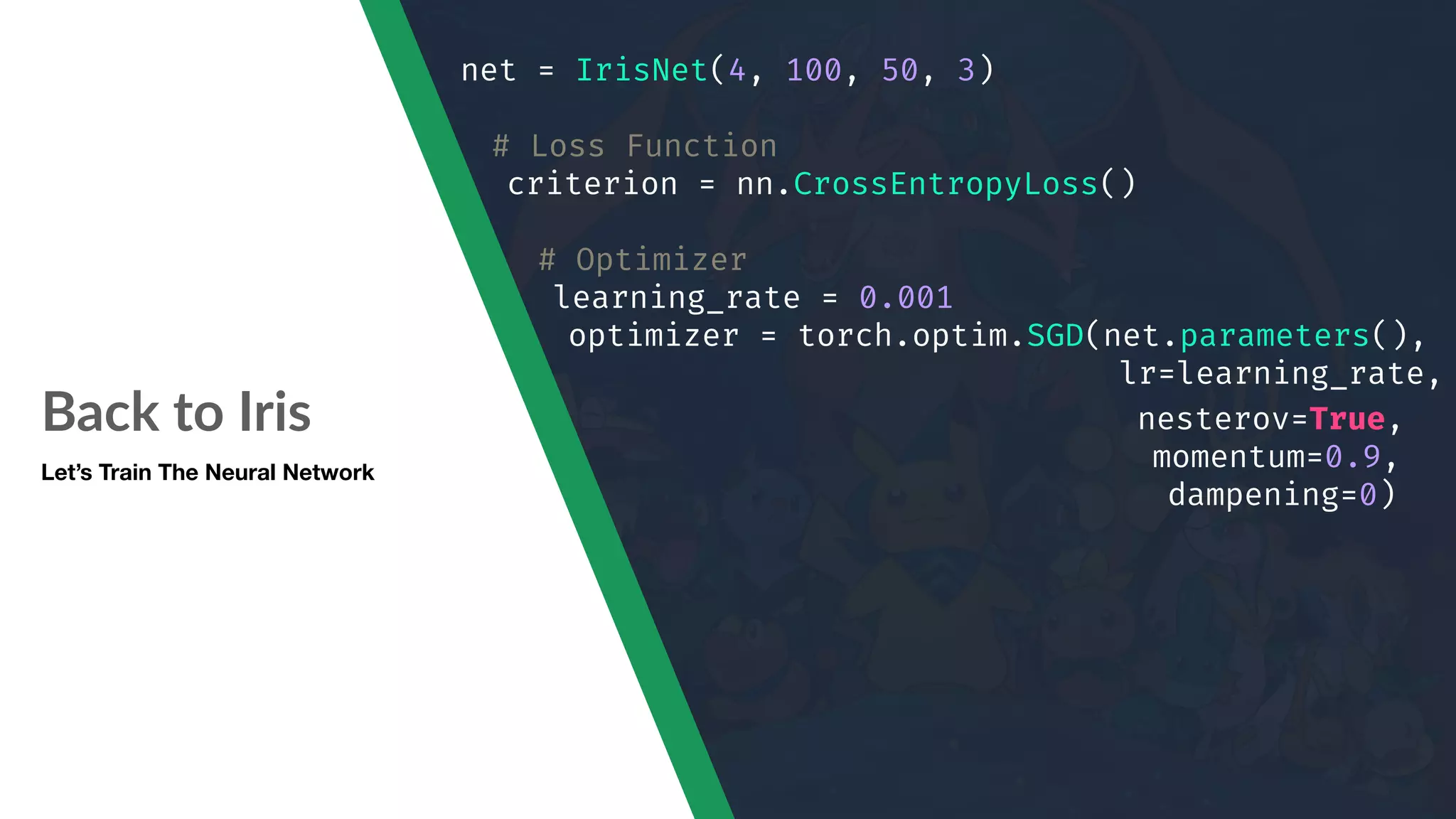
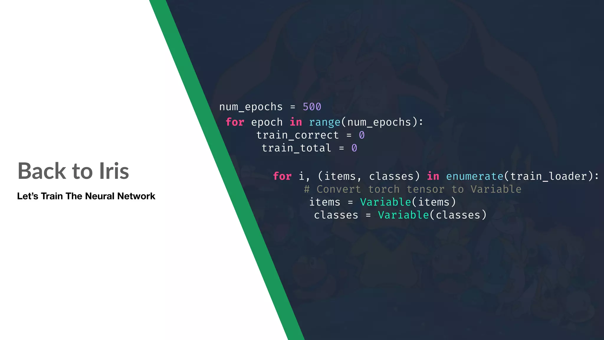
![Back to Iris Let’s Train The Neural Network import torch import torch.nn as nn import matplotlib.pyplot as plt from torch.autograd import Variable from data import iris # Create the module class IrisNet(nn.Module): def "__init"__(self, input_size, hidden1_size, hidden2_size, num_classes): super(IrisNet, self)."__init"__() self.layer1 = nn.Linear(input_size, hidden1_size) self.act1 = nn.ReLU() self.layer2 = nn.Linear(hidden1_size, hidden2_size) self.act2 = nn.ReLU() self.layer3 = nn.Linear(hidden2_size, num_classes) def forward(self, x): out = self.layer1(x) out = self.act1(out) out = self.layer2(out) out = self.act2(out) out = self.layer3(out) return out # Create a model instance model = IrisNet(4, 100, 50, 3) print(model) # Create the DataLoader batch_size = 60 iris_data_file = 'data/iris.data.txt' train_ds, test_ds = iris.get_datasets(iris_data_file) print('# instances in training set: ', len(train_ds)) print('# instances in testing/validation set: ', len(test_ds)) train_loader = torch.utils.data.DataLoader(dataset=train_ds, batch_size=batch_size, shuffle=True) test_loader = torch.utils.data.DataLoader(dataset=test_ds, batch_size=batch_size, shuffle=True) # Model net = IrisNet(4, 100, 50, 3) # Loss Function criterion = nn.CrossEntropyLoss() # Optimizer learning_rate = 0.001 optimizer = torch.optim.SGD(net.parameters(), lr=learning_rate, nesterov=True, momentum=0.9, dampening=0) # Training iteration num_epochs = 500 train_loss = [] test_loss = [] train_accuracy = [] test_accuracy = [] for epoch in range(num_epochs): train_correct = 0 train_total = 0 for i, (items, classes) in enumerate(train_loader): # Convert torch tensor to Variable items = Variable(items) classes = Variable(classes) net.train() # Training mode optimizer.zero_grad() # Reset gradients from past operation outputs = net(items) # Forward pass loss = criterion(outputs, classes) # Calculate the loss loss.backward() # Calculate the gradient optimizer.step() # Adjust weight/parameter based on gradients train_total += classes.size(0) _, predicted = torch.max(outputs.data, 1) train_correct += (predicted "== classes.data).sum() print('Epoch %d/%d, Iteration %d/%d, Loss: %.4f' %(epoch+1, num_epochs, i+1, len(train_ds)"//batch_size, loss.data[0])) net.eval() # Put the network into evaluation mode train_loss.append(loss.data[0]) train_accuracy.append((100 * train_correct / train_total)) # Record the testing loss test_items = torch.FloatTensor(test_ds.data.values[:, 0:4]) test_classes = torch.LongTensor(test_ds.data.values[:, 4]) outputs = net(Variable(test_items)) loss = criterion(outputs, Variable(test_classes)) test_loss.append(loss.data[0]) # Record the testing accuracy _, predicted = torch.max(outputs.data, 1) total = test_classes.size(0) correct = (predicted "== test_classes).sum() test_accuracy.append((100 * correct / total))](https://image.slidesharecdn.com/machinelearningwithpytorch-181012233426/75/Machine-learning-with-py-torch-67-2048.jpg)


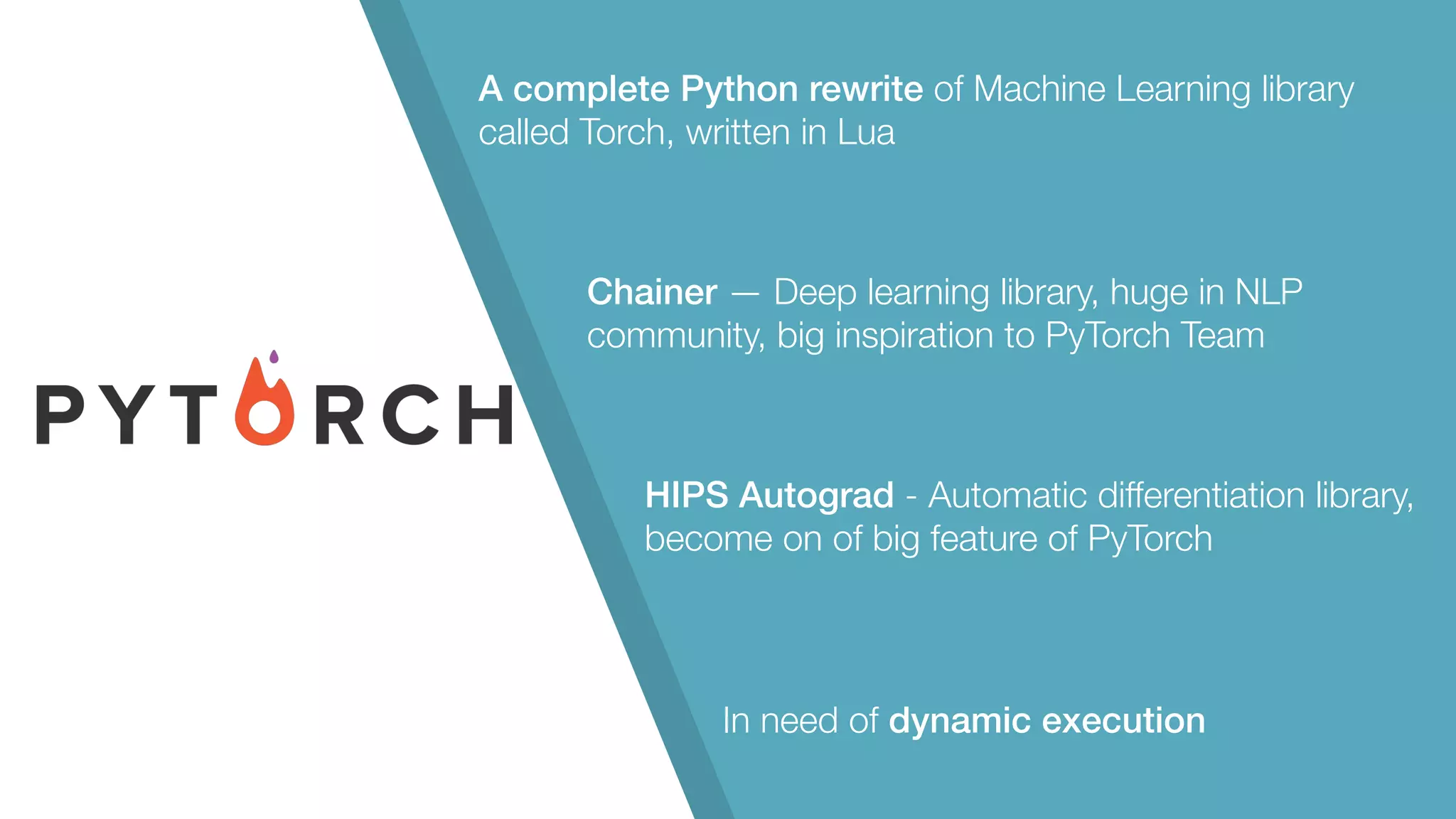
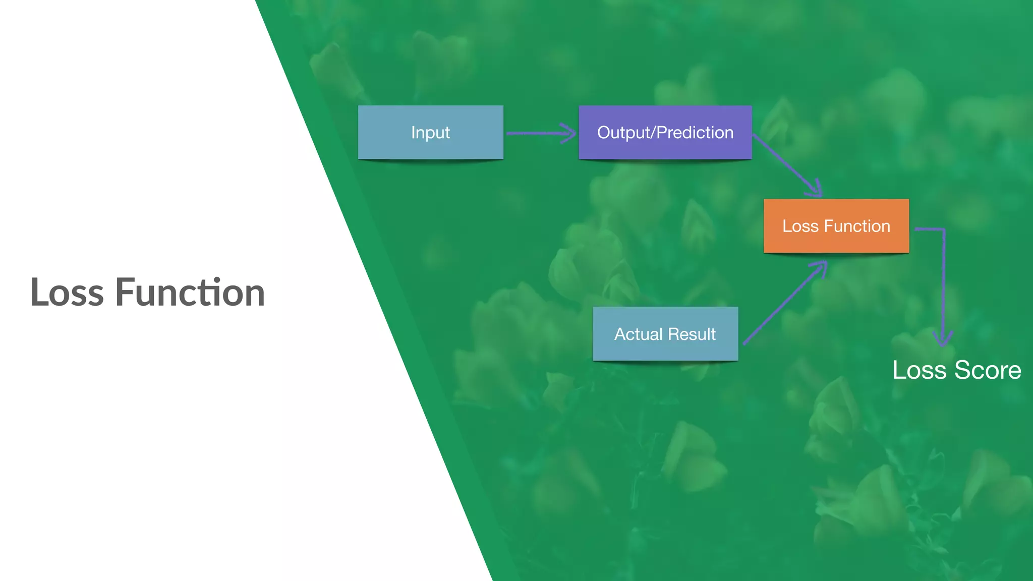
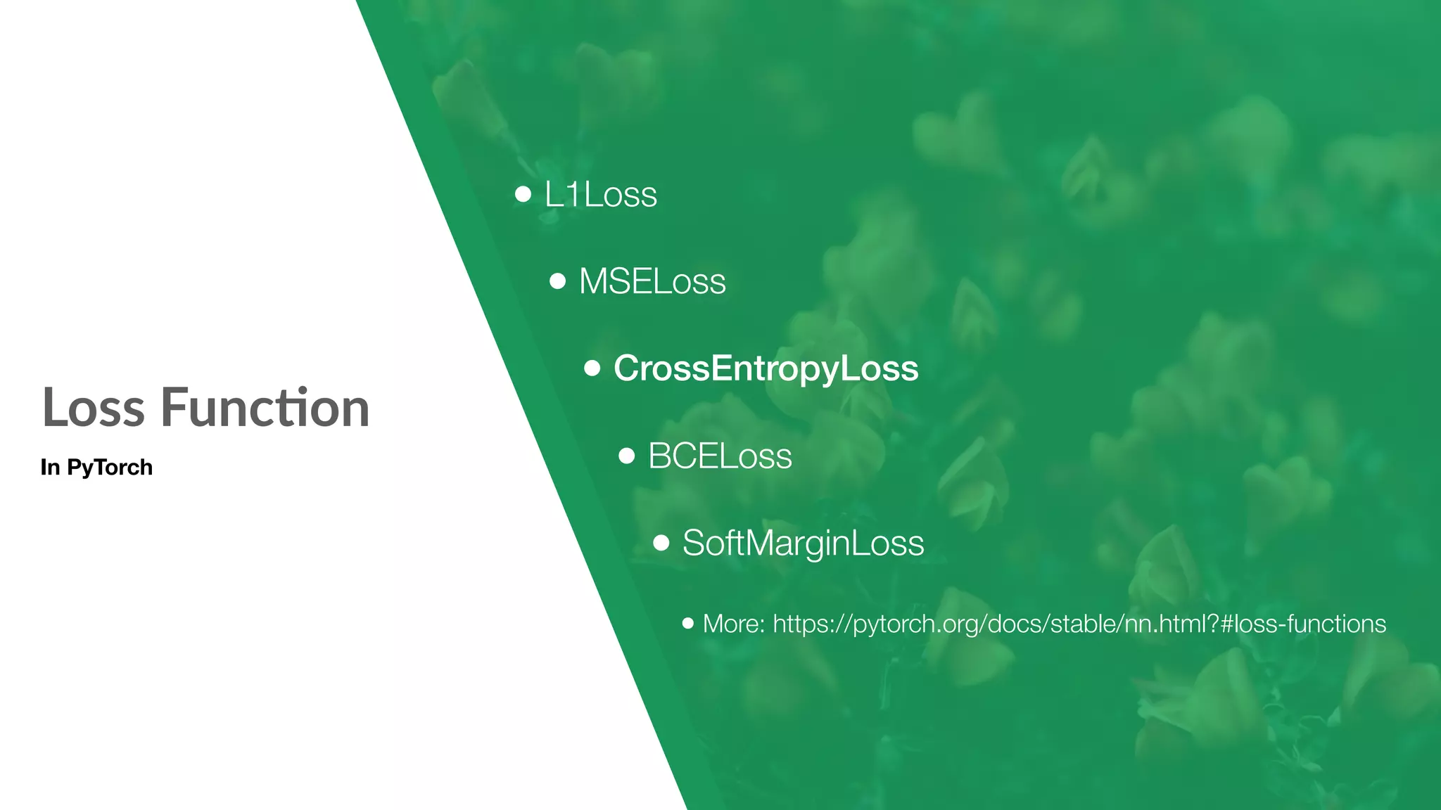
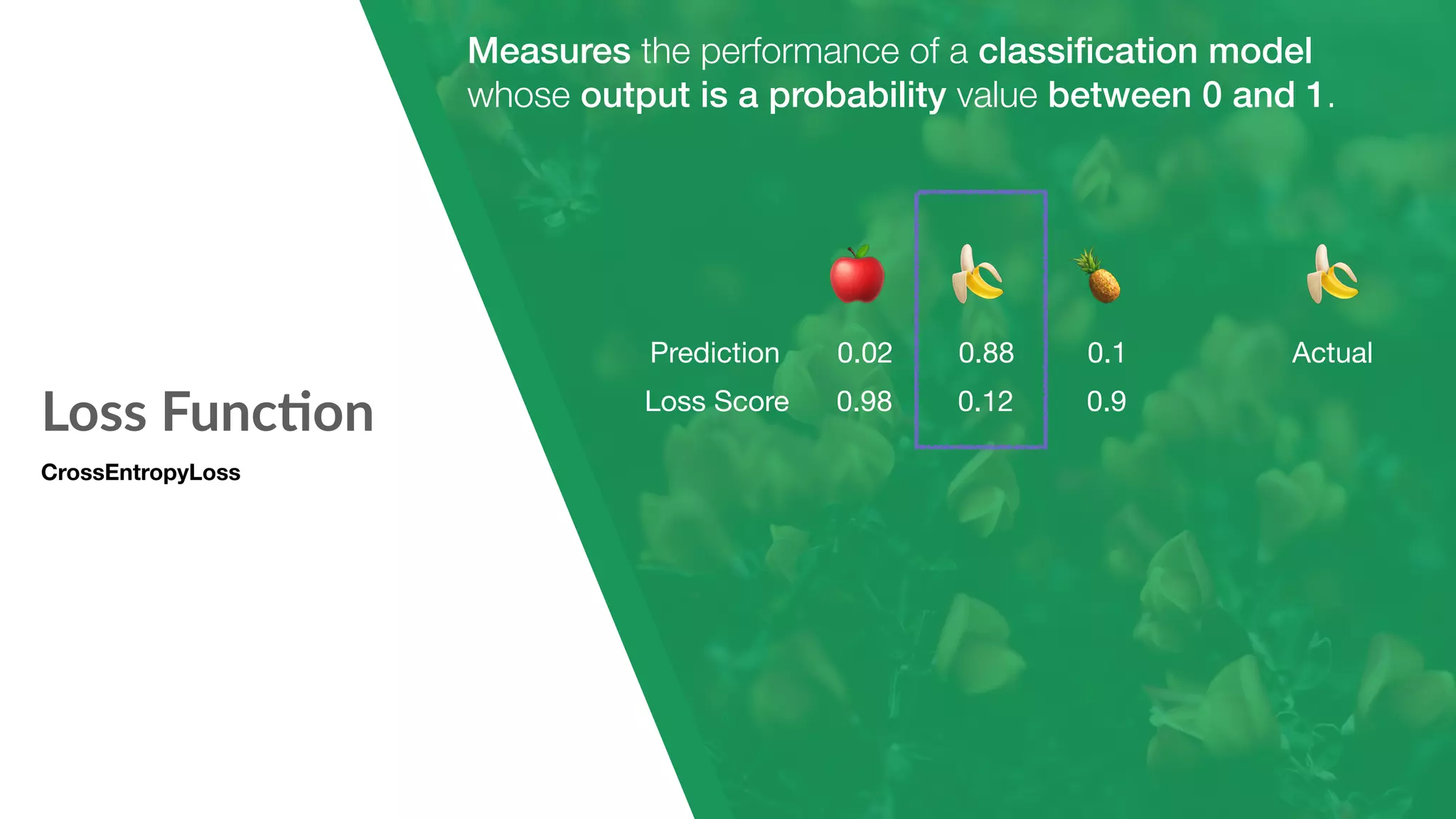
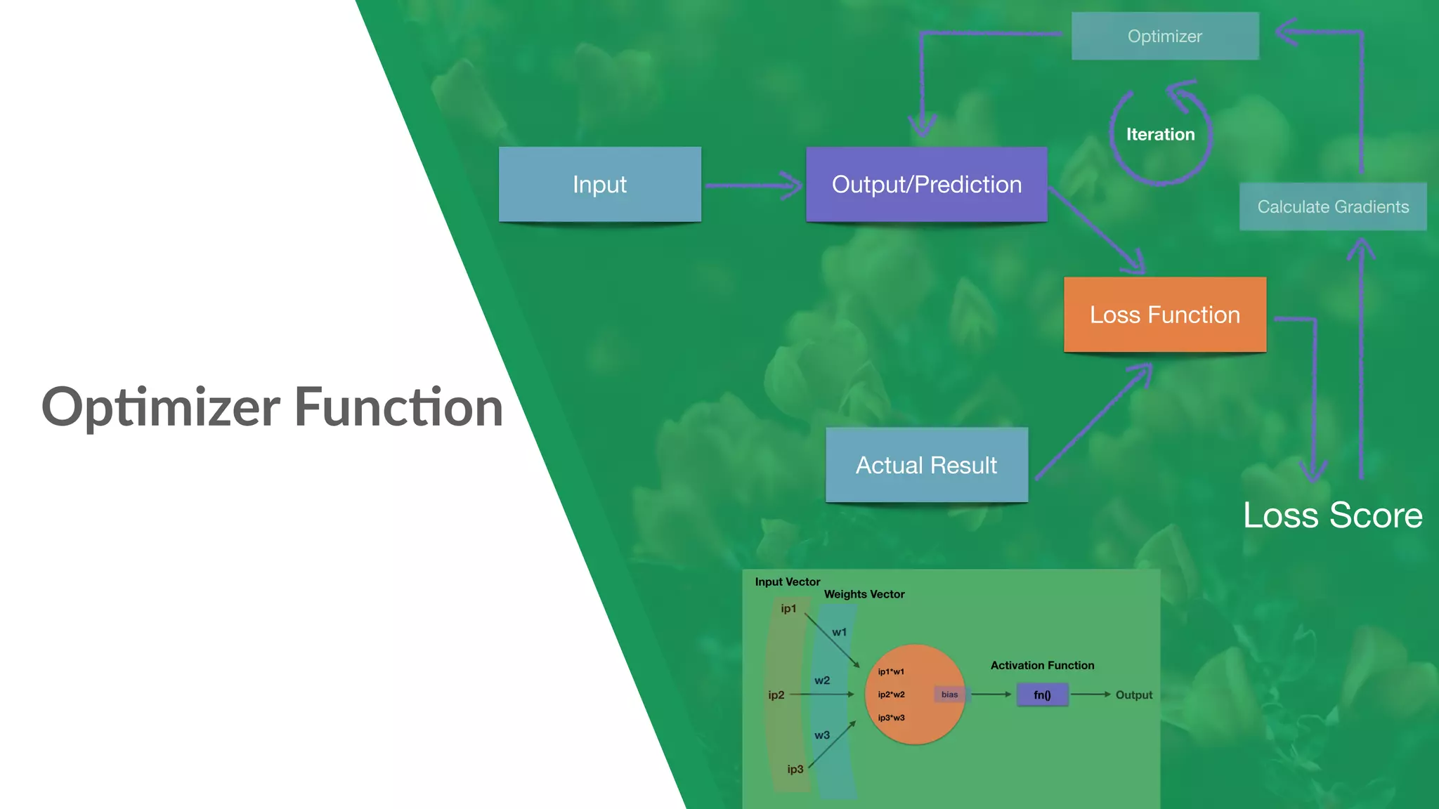
The document provides a comprehensive introduction to PyTorch, a Python machine learning library focused on research and dynamic computation, showcasing its features, installation, handling datasets, and building neural networks. It covers basic concepts such as tensors, autograd for automatic differentiation, and hands-on examples like creating a feedforward neural network to classify the iris dataset. Additionally, it discusses loss functions and optimization techniques for training models in PyTorch.
Introduction to PyTorch with history, features, and its use in machine learning.
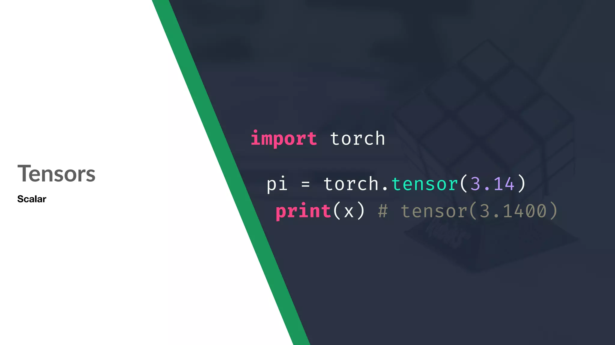
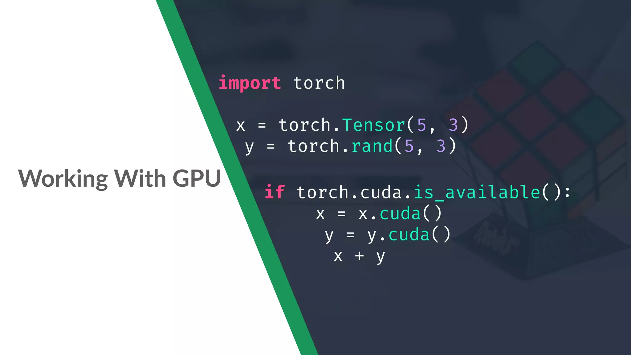
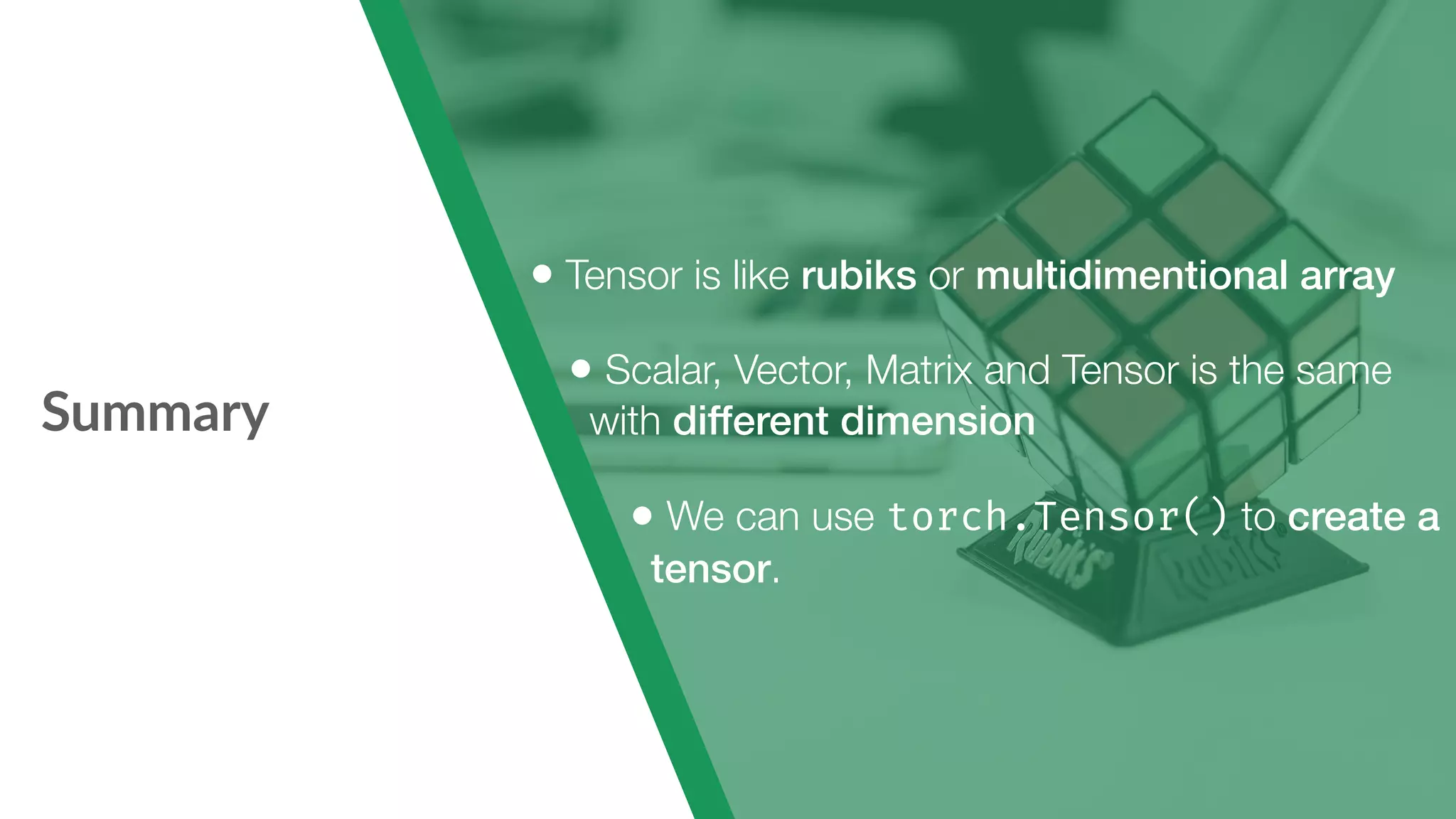
Installation, usage of tensors, and basic operations in PyTorch.
Concept of automatic differentiation in PyTorch, the role of Variable, and the autograd module.
Explanation of datasets, epochs, batches, iterations, and example datasets like CIFAR10.
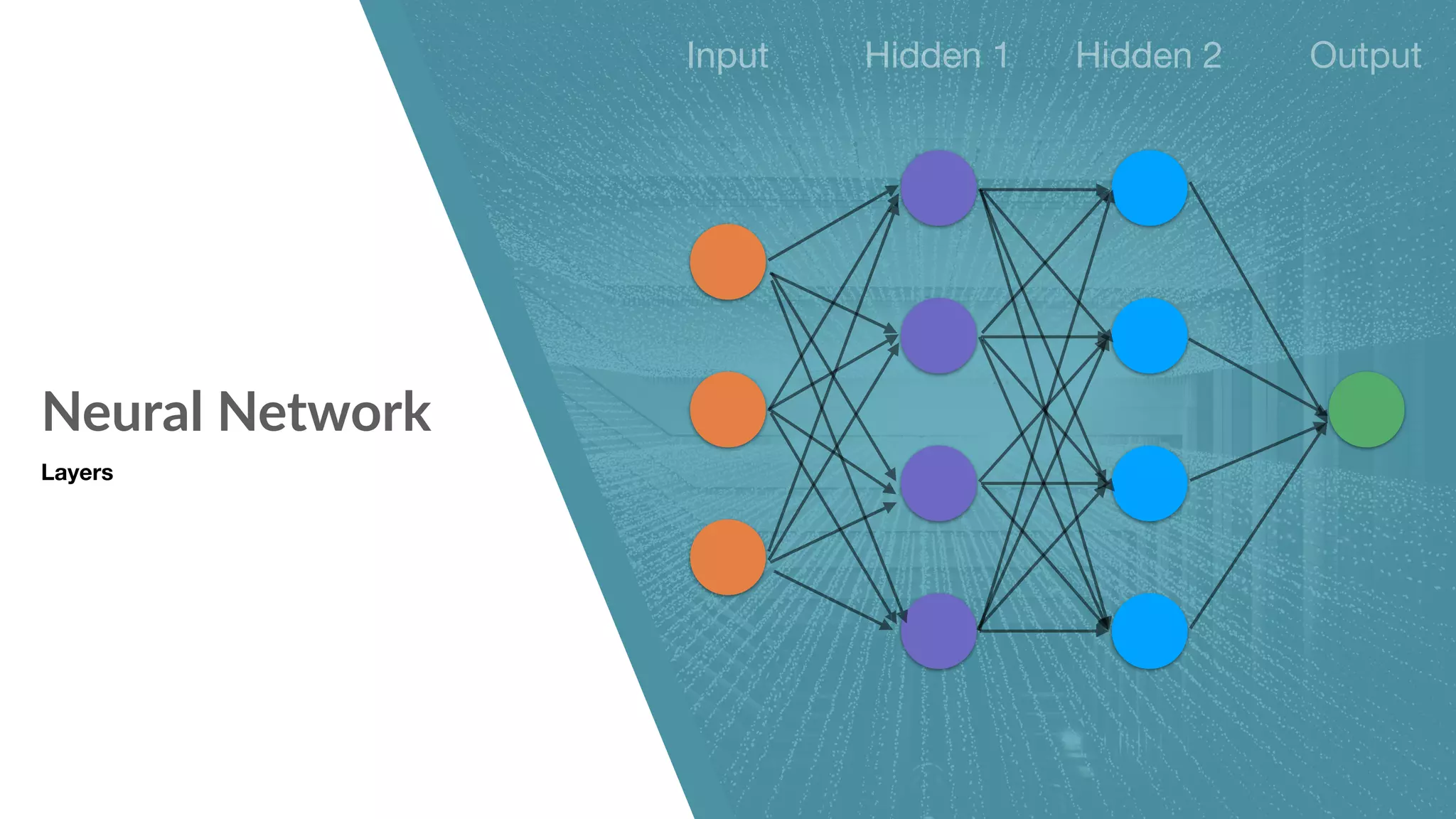
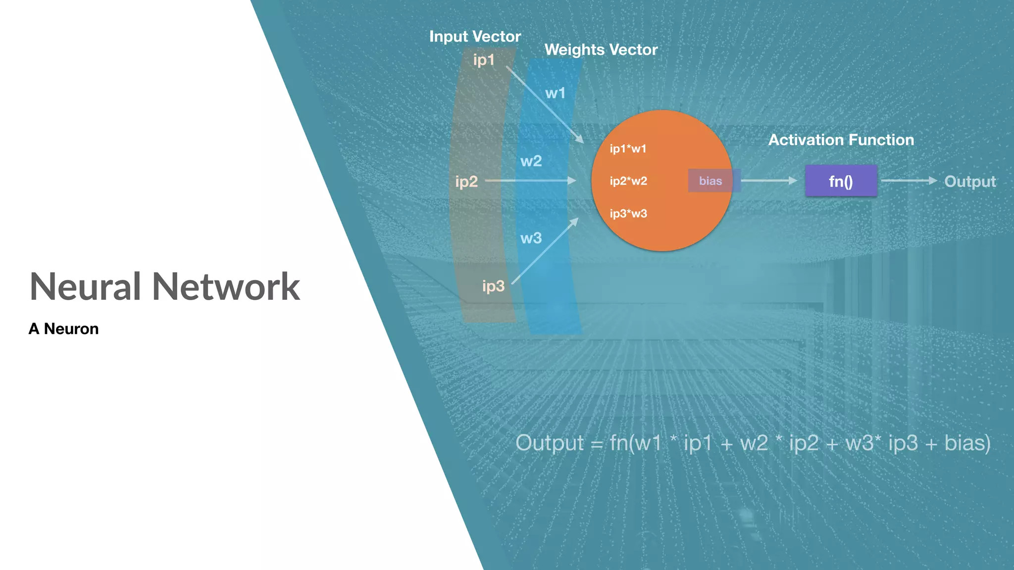
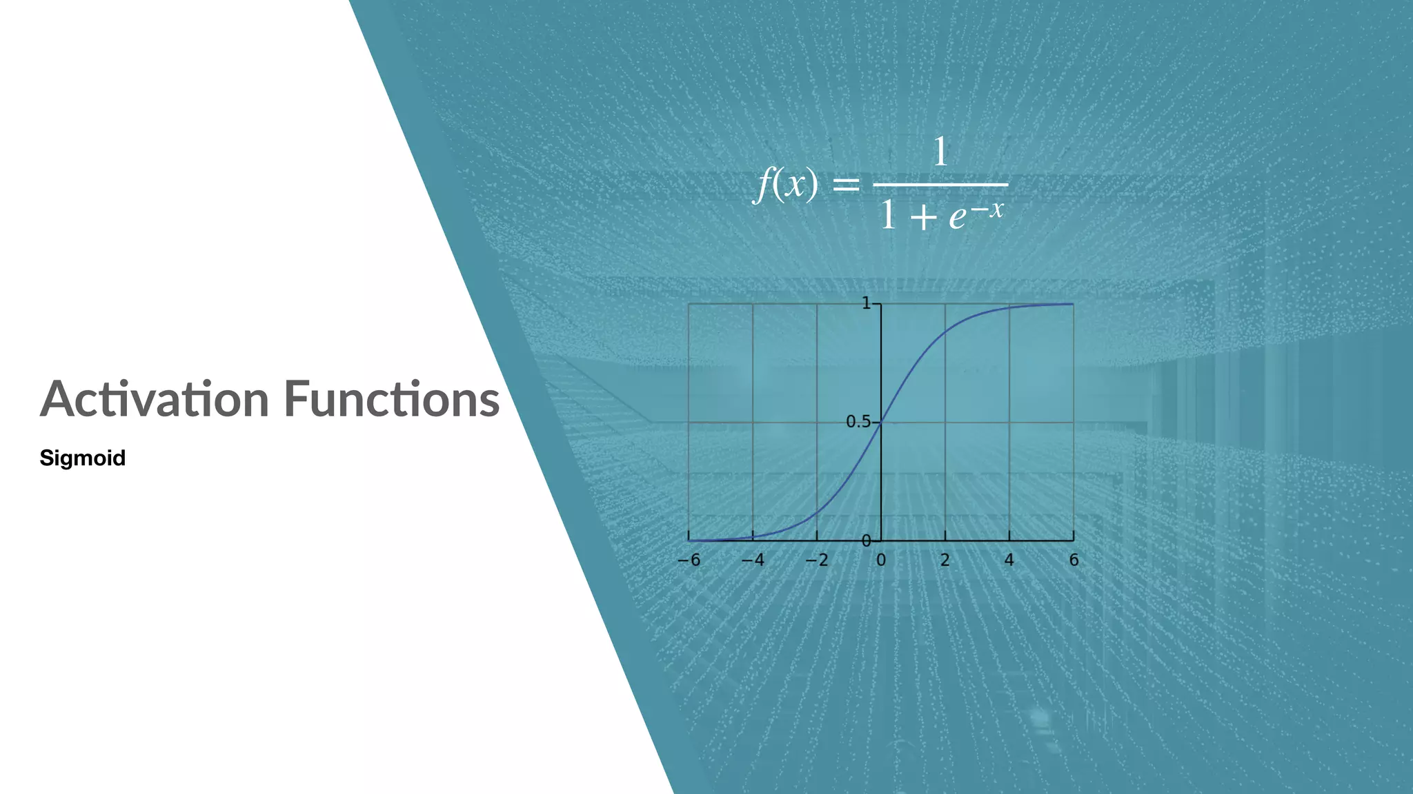
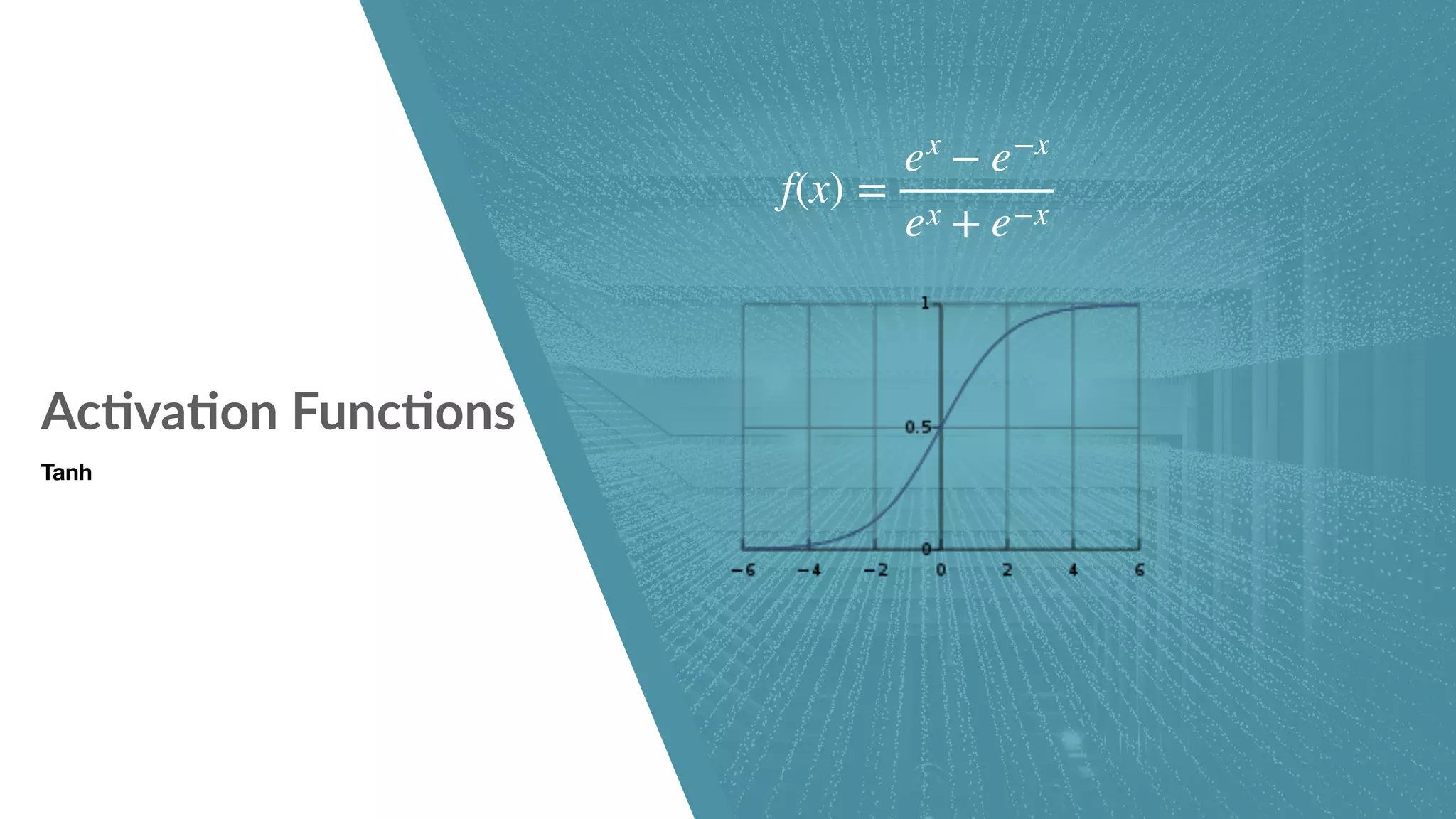
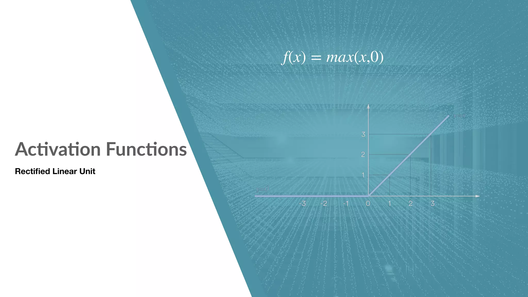
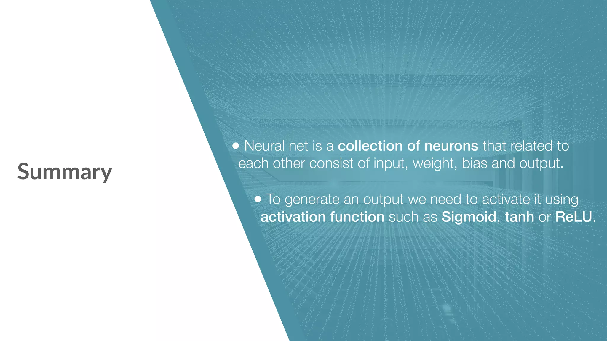
Neural network structure and components including activation functions.
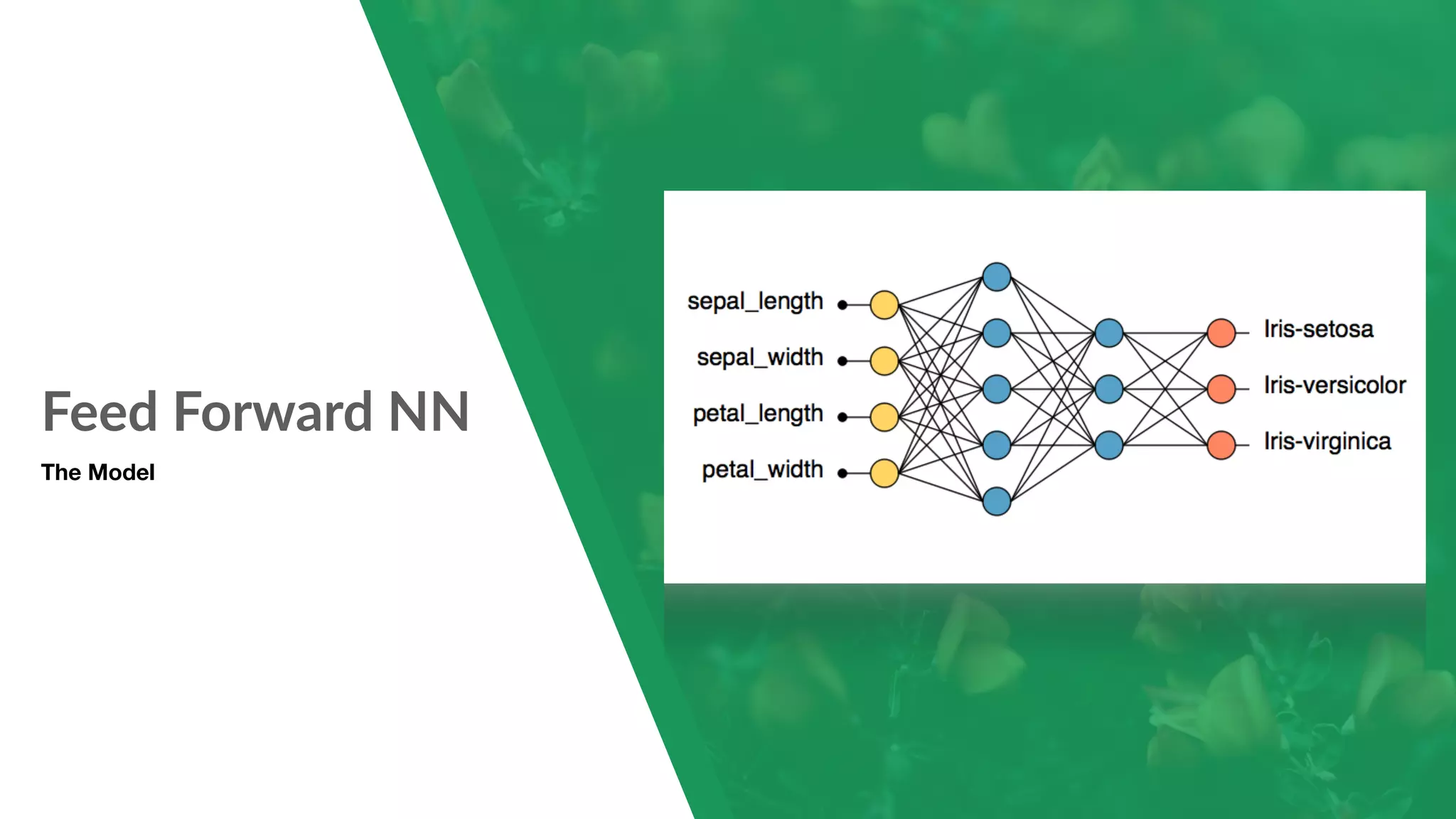
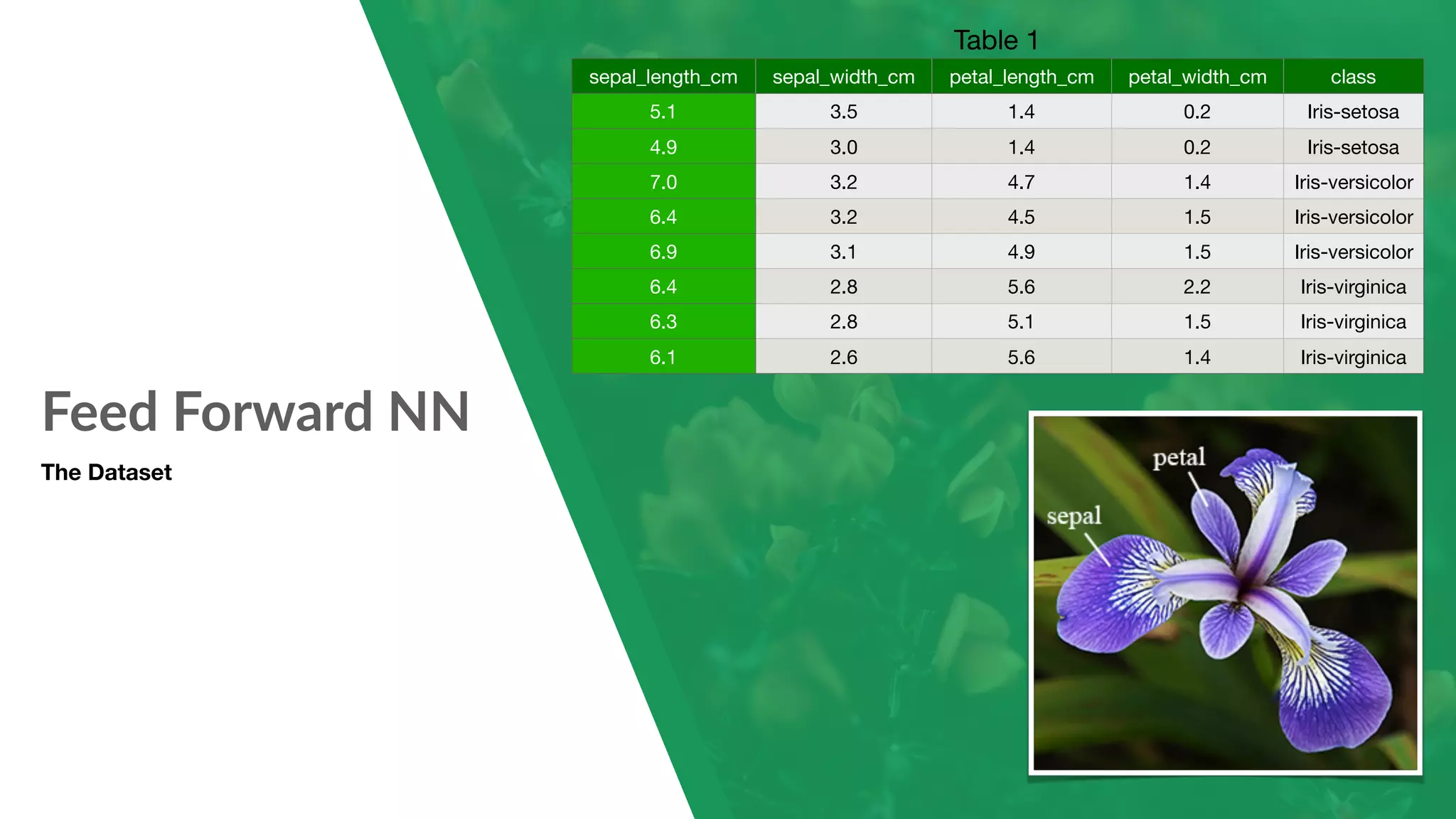
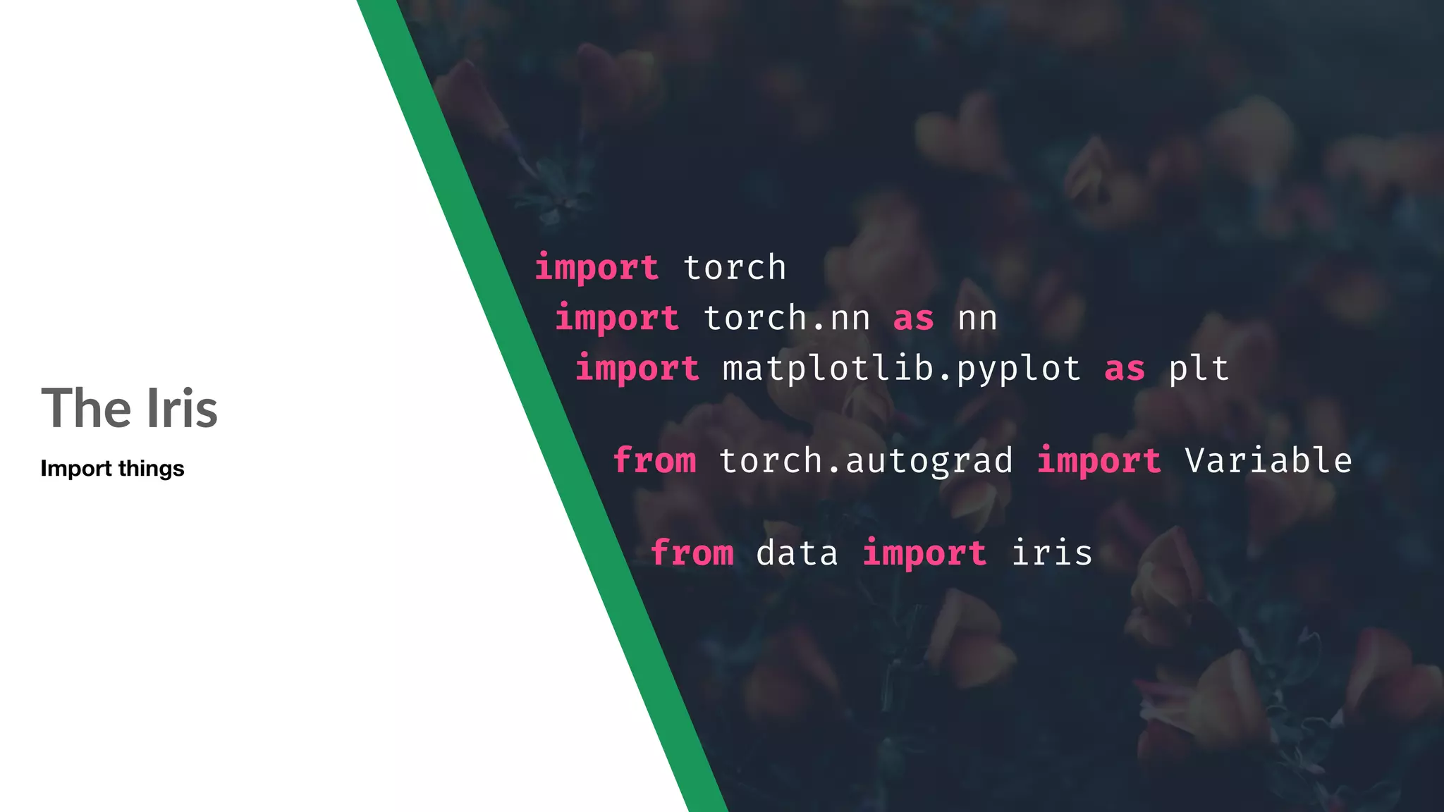
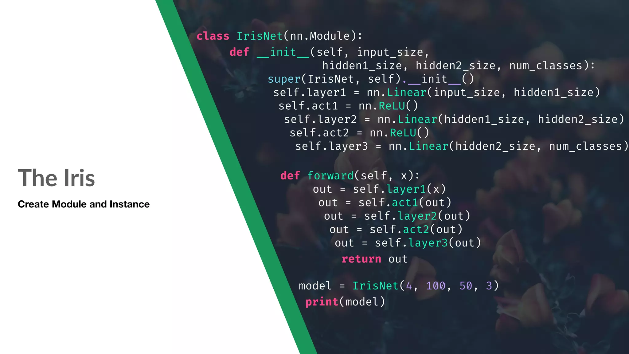
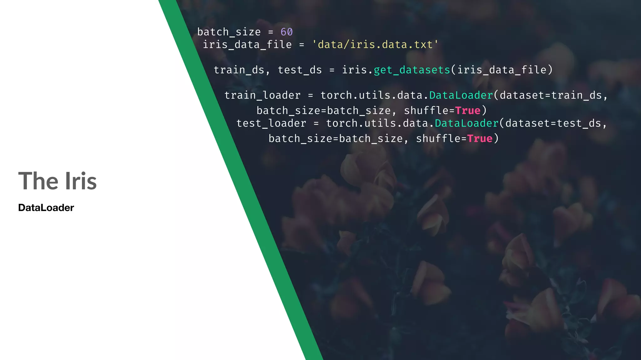
Implementation of a feed-forward neural network to classify flower types using the Iris dataset.
Suggestions for further resources and personal contact information.