This document provides information about neural networks from Parveen Malik, an Assistant Professor at KIIT University. It defines a neural network as a massively parallel distributed processor made up of simple processing units that has a natural ability to store experiential knowledge and make it available for use, similar to the human brain. Neural networks can be used for applications like object detection, image captioning, time series modelling, and more. The document also discusses the structure and function of biological neurons and their equivalence to artificial neurons in neural networks.
Parveen Malik introduces neural networks at KIIT University. Textbooks such as Haykin's 'Neural Networks and Learning Machines' are listed.
A neural network is defined as a processor similar to the brain, learning through experience by adjusting connection strengths (synaptic weights).
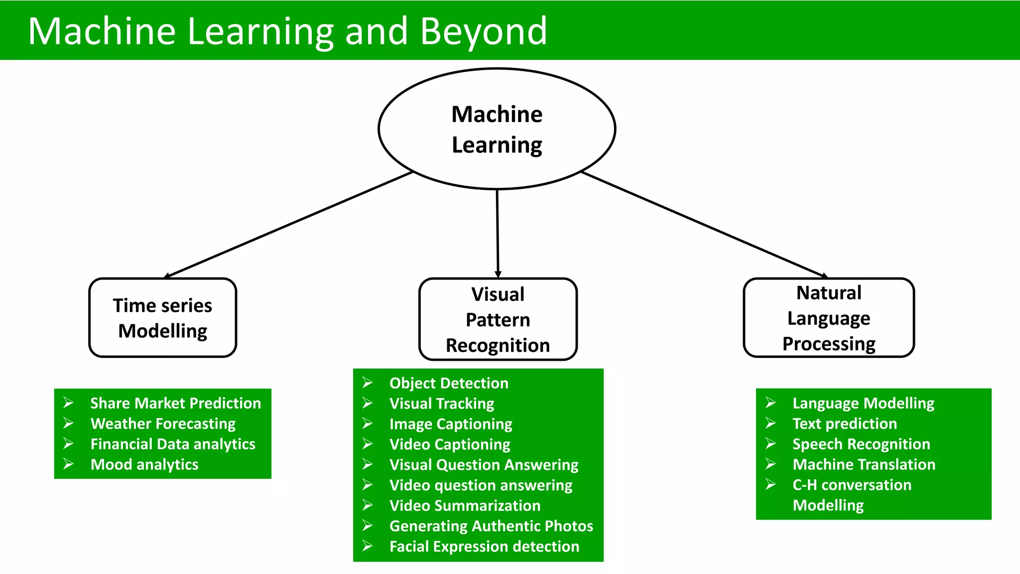
Neural networks are essential in machine learning applications like object detection, visual tracking, and financial analytics.
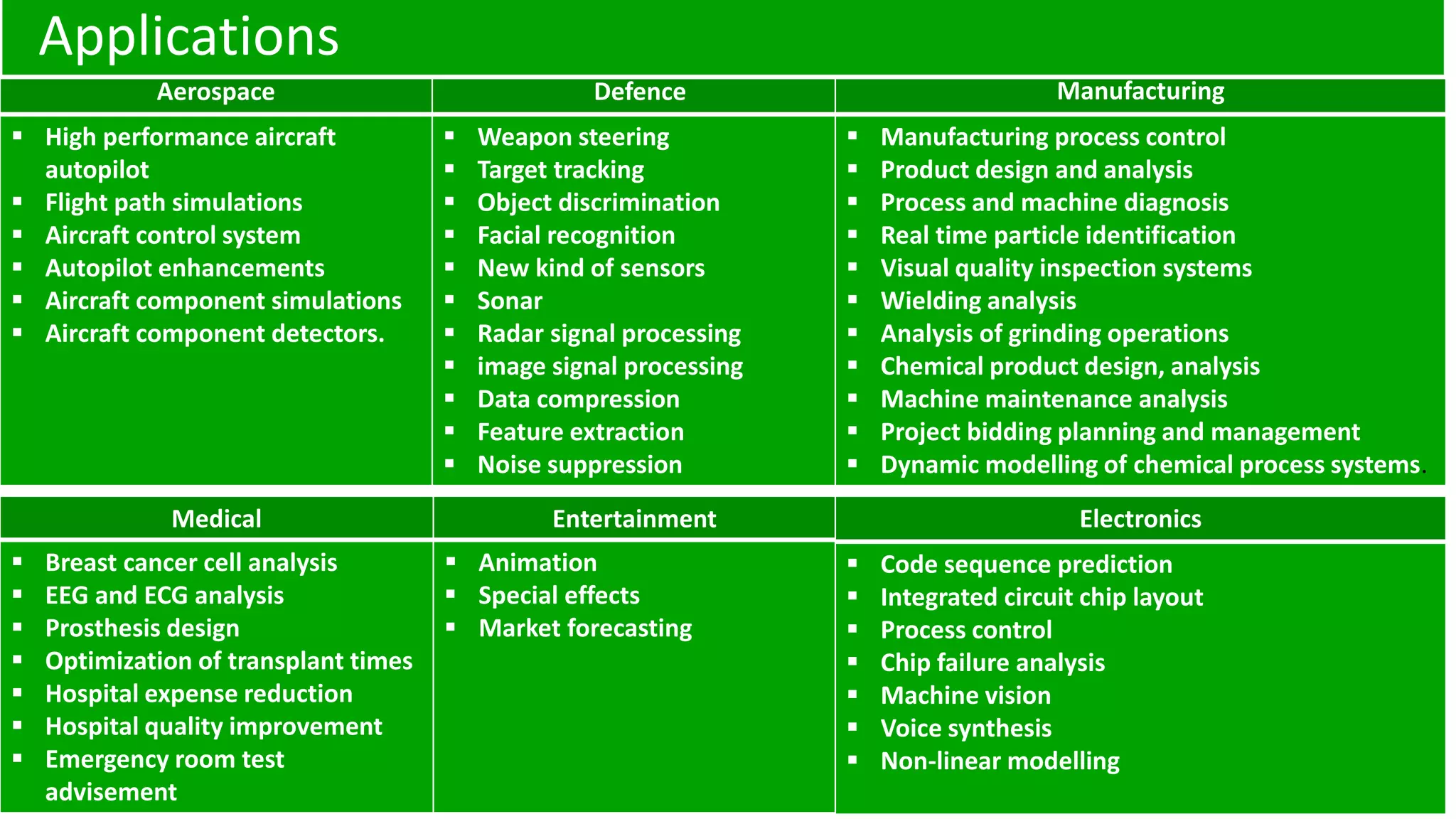
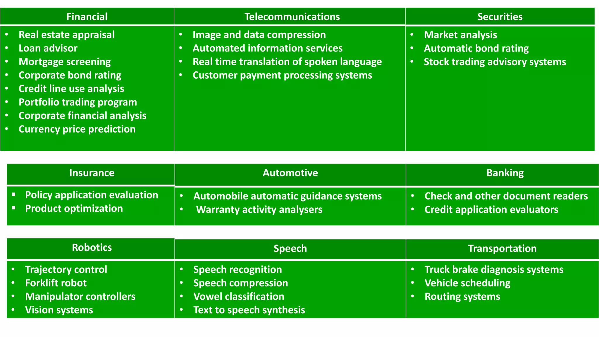
Various sectors benefit from neural networks, including aerospace, medical, manufacturing, telecommunications, and banking, enhancing capabilities in each field.
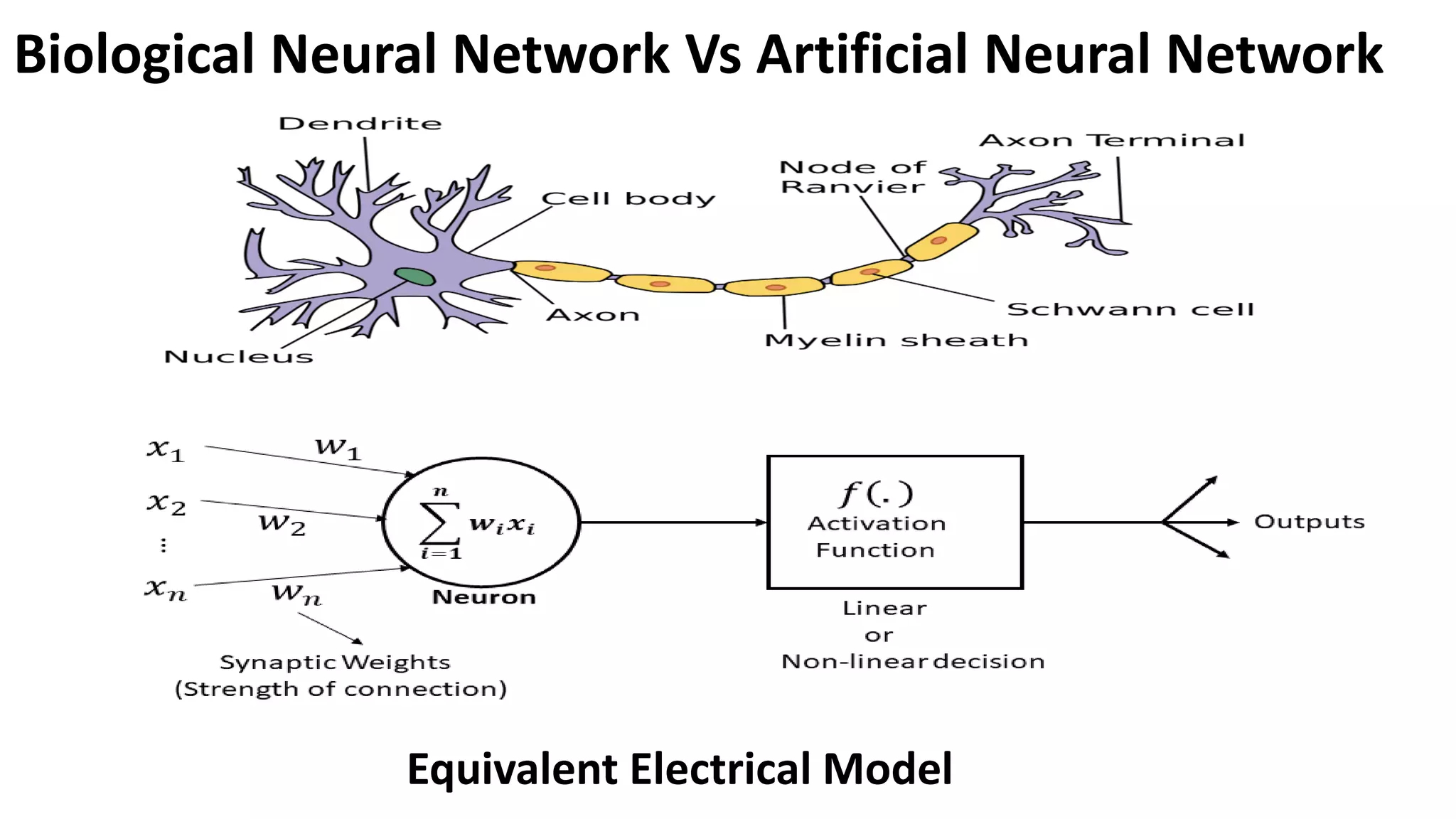
Comparison between human neurons and artificial neurons, emphasizing structure, functioning, and properties of biological neural networks.
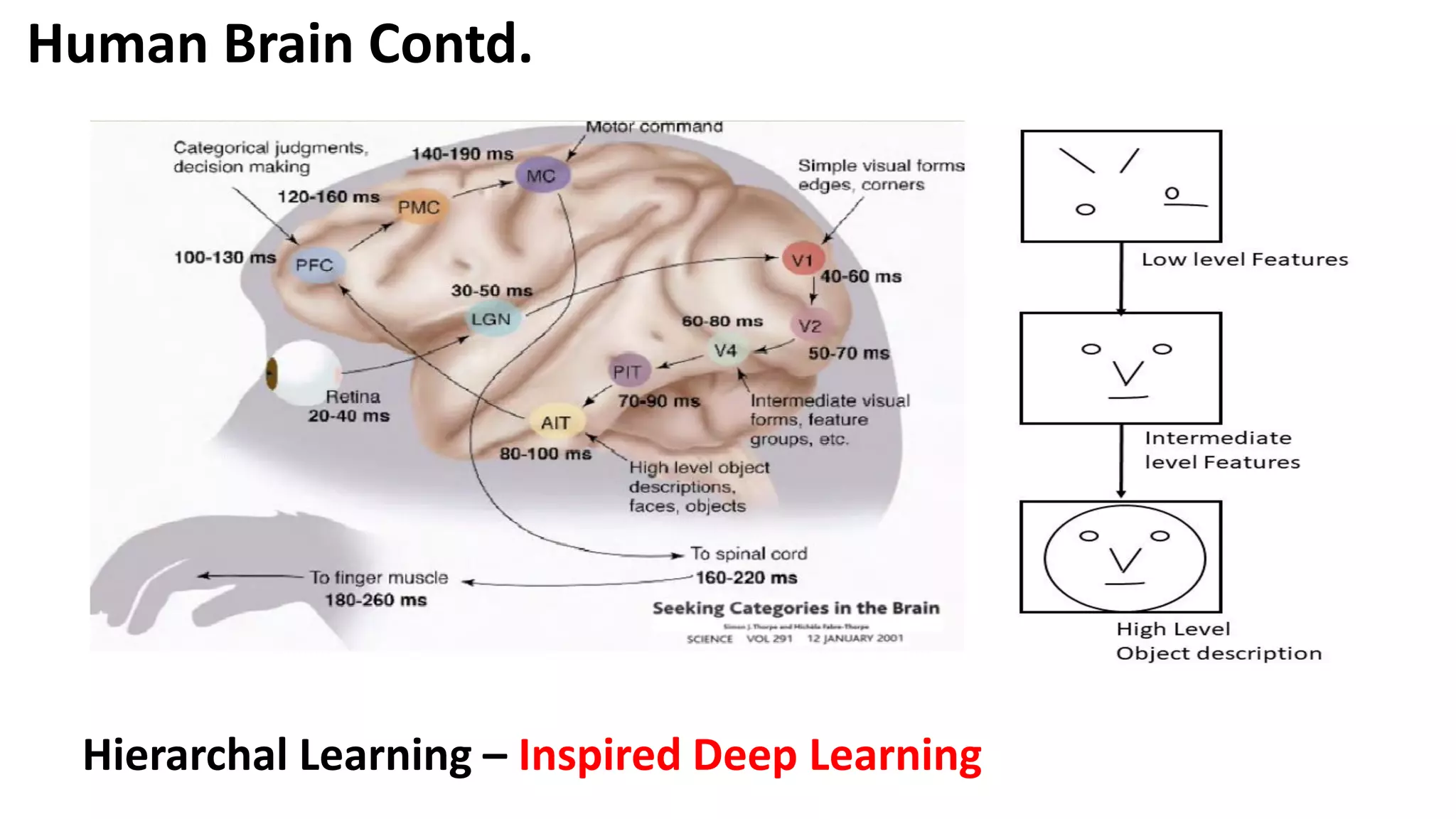
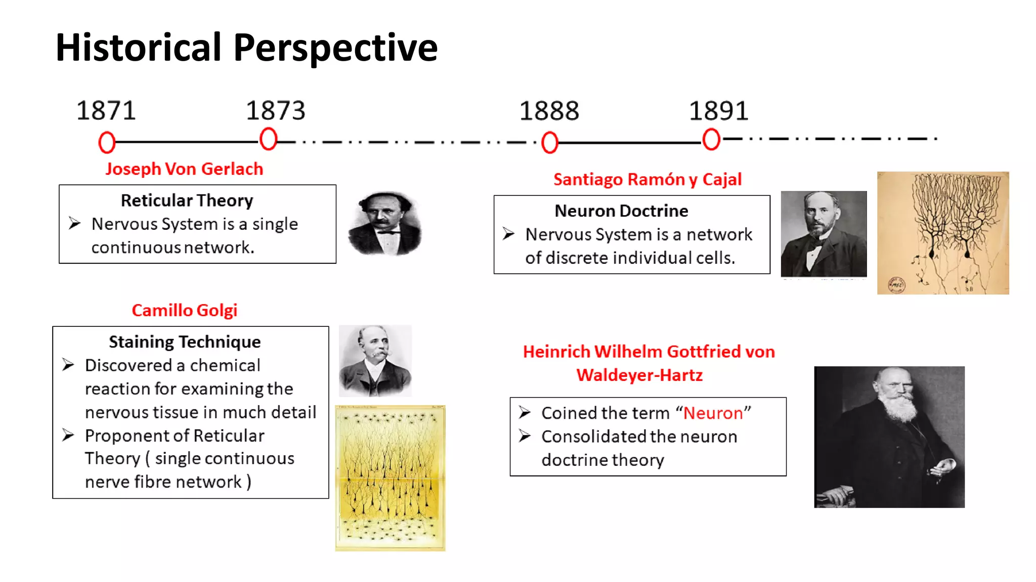
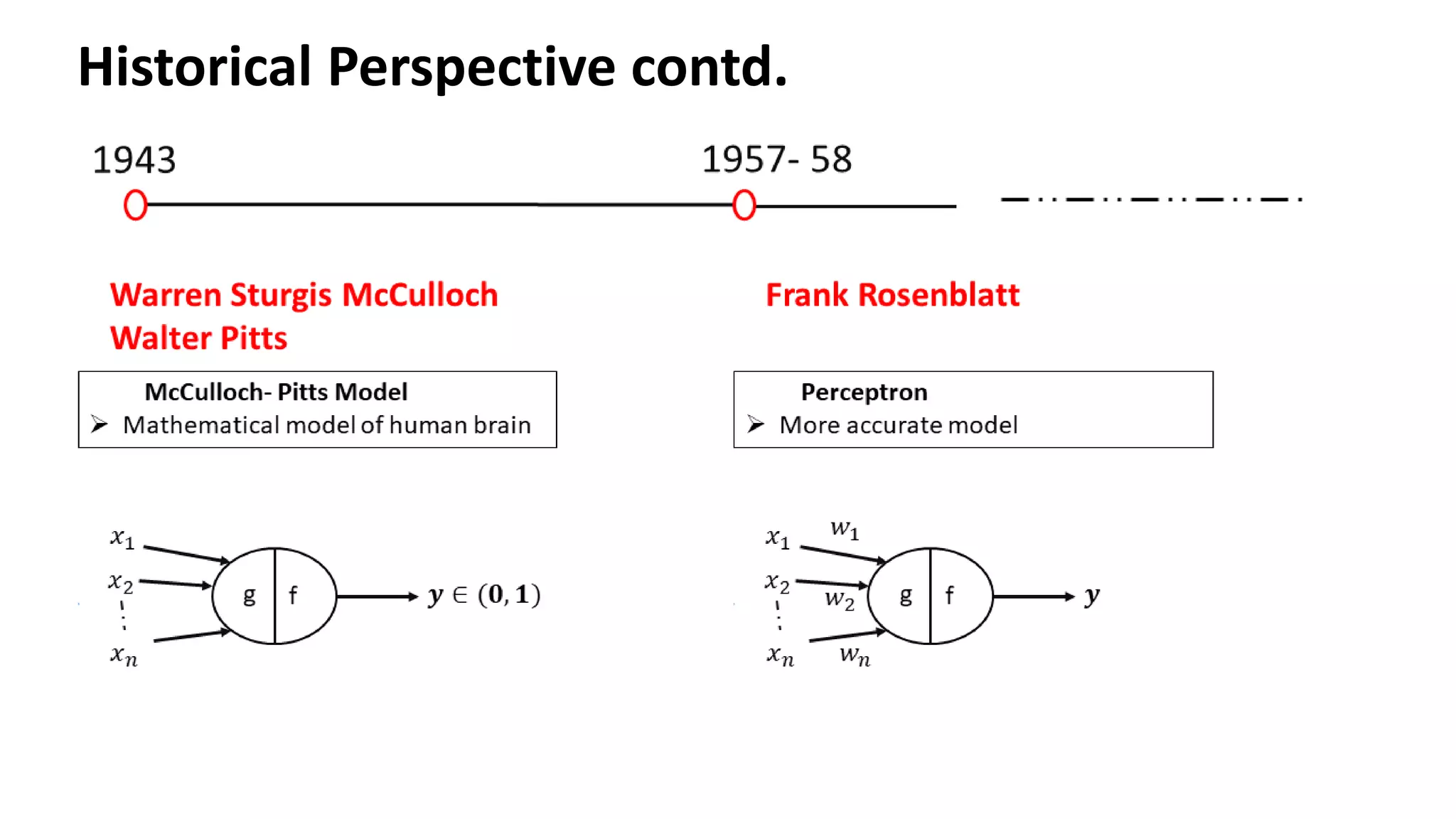
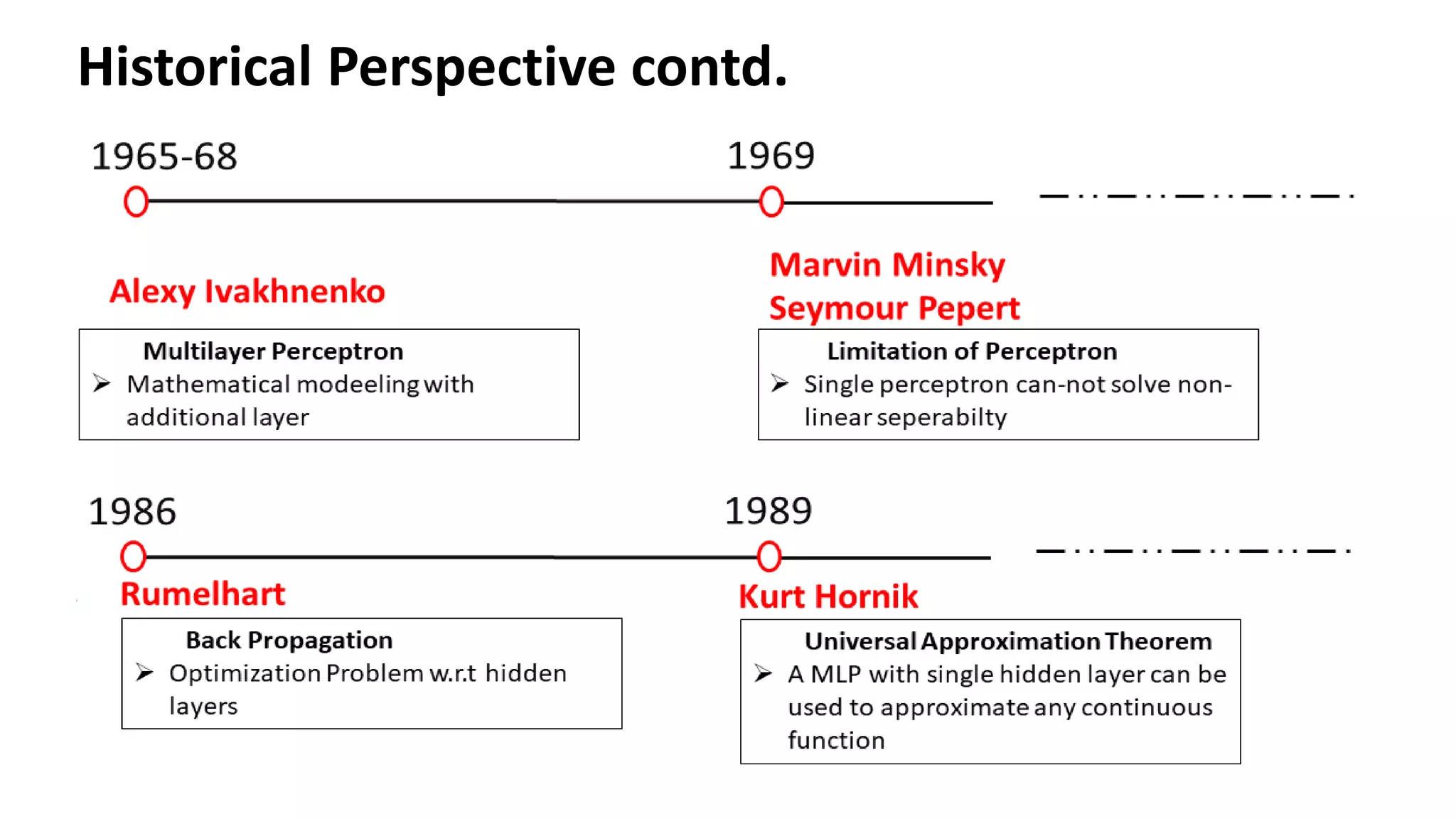
Overview of the evolution of neural network models inspired by human brain functions, highlighting key historical contributions.
Outlines practical models of neural networks, activation functions, and learning rules such as Hebbian and Perceptron learning rules. Details on Hebbian and Perceptron learning rules focusing on updating weights for classification tasks with implementation examples.
Text Books: • NeuralNetworks and Learning Machines – Simon Haykin • Principles of Soft Computing- S.N.Shivnandam & S.N.Deepa • Neural Networks using Matlab- S.N. Shivanandam, S. Sumathi ,S N Deepa
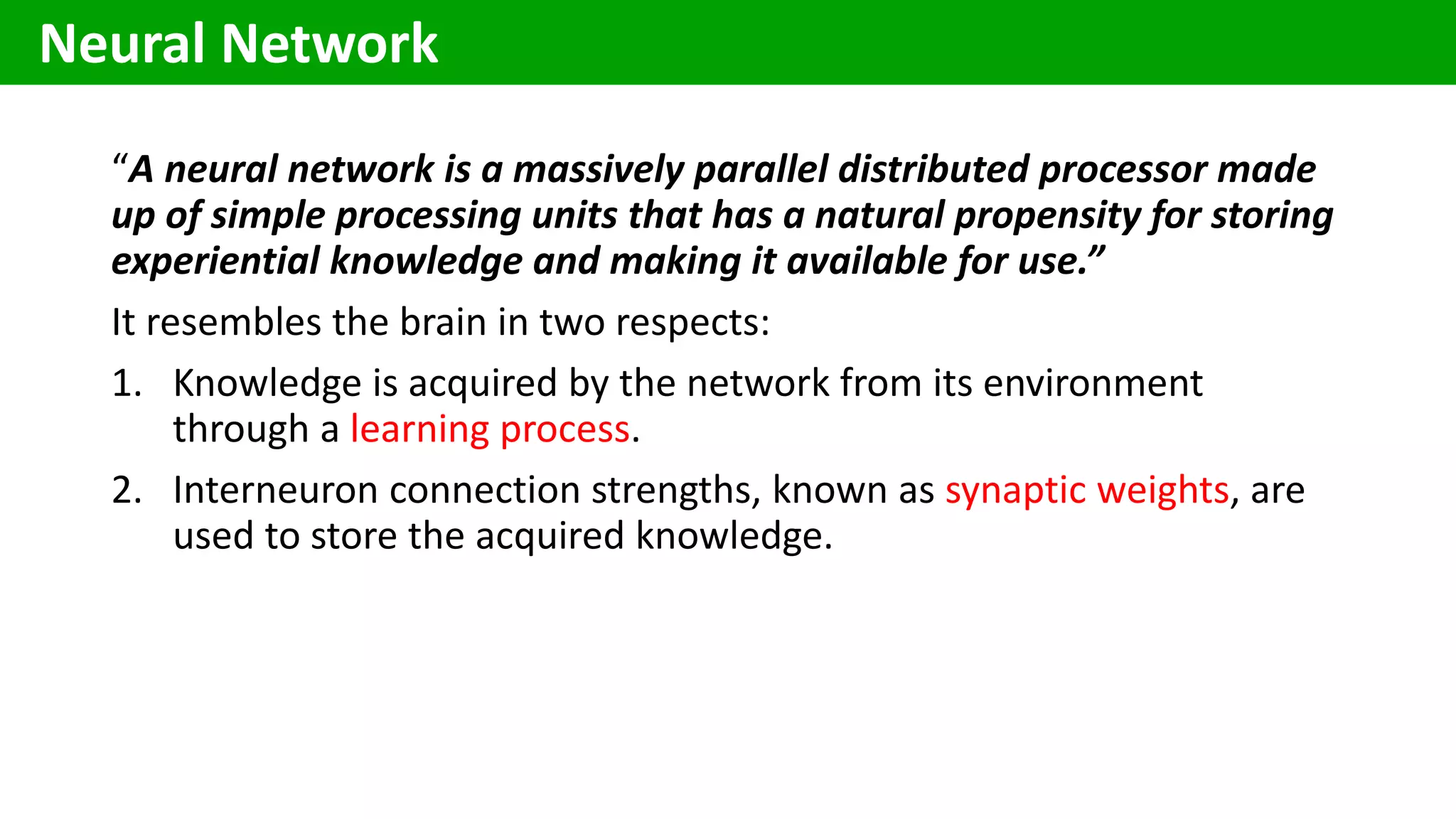
“A neural networkis a massively parallel distributed processor made up of simple processing units that has a natural propensity for storing experiential knowledge and making it available for use.” It resembles the brain in two respects: 1. Knowledge is acquired by the network from its environment through a learning process. 2. Interneuron connection strengths, known as synaptic weights, are used to store the acquired knowledge. Neural Network
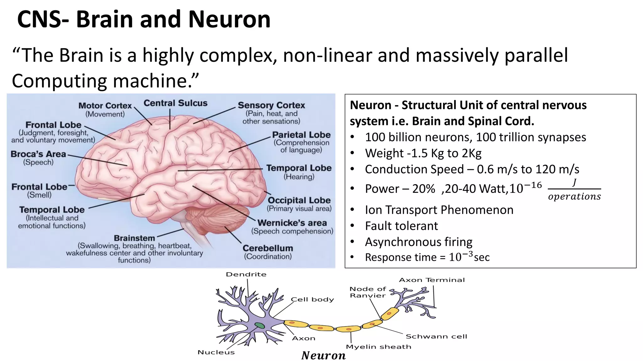
CNS- Brain andNeuron Neuron - Structural Unit of central nervous system i.e. Brain and Spinal Cord. • 100 billion neurons, 100 trillion synapses • Weight -1.5 Kg to 2Kg • Conduction Speed – 0.6 m/s to 120 m/s • Power – 20% ,20-40 Watt,10−16 𝐽 𝑜𝑝𝑒𝑟𝑎𝑡𝑖𝑜𝑛𝑠 • Ion Transport Phenomenon • Fault tolerant • Asynchronous firing • Response time = 10−3 sec “The Brain is a highly complex, non-linear and massively parallel Computing machine.” 𝑵𝒆𝒖𝒓𝒐𝒏
12.
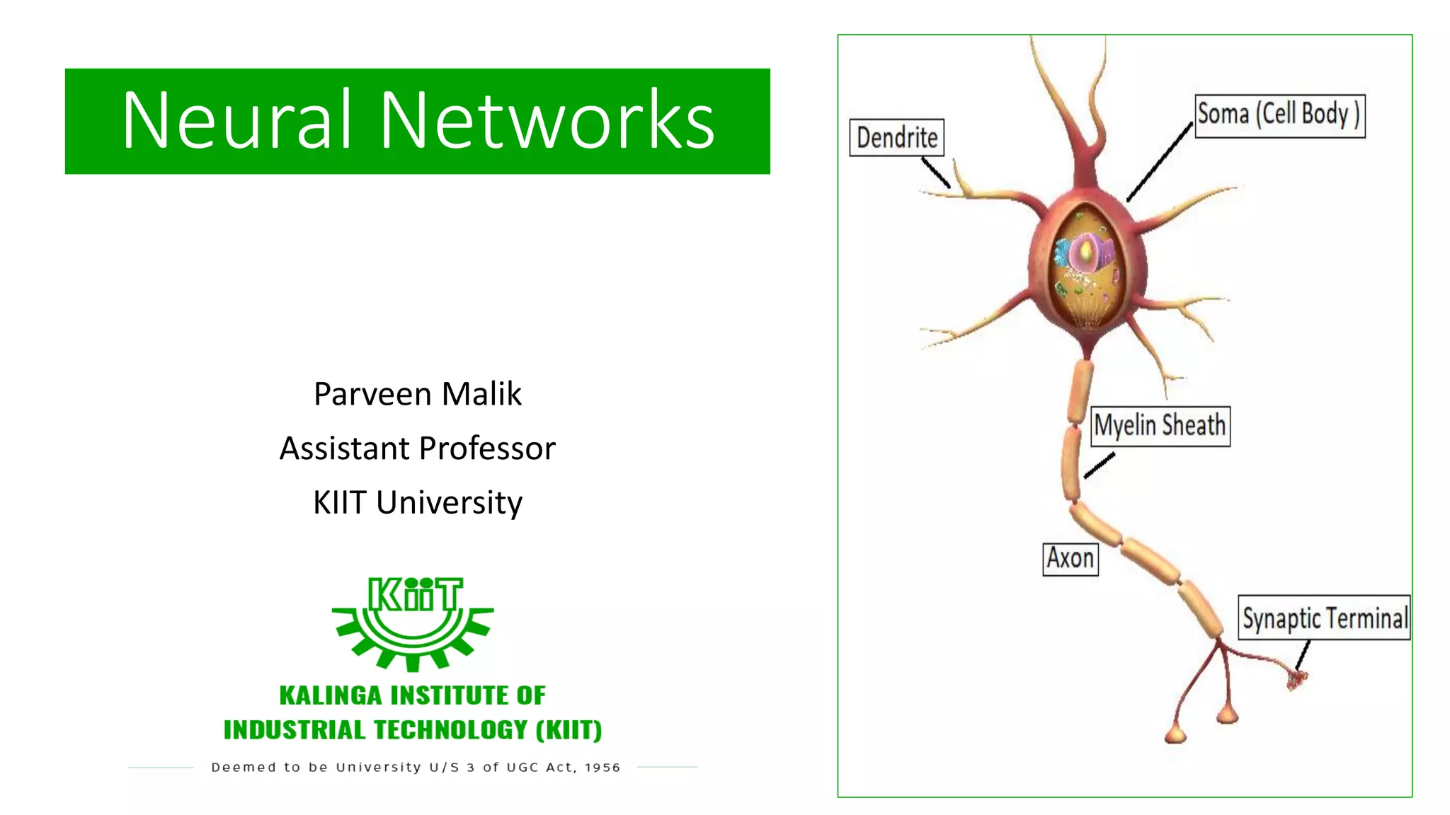
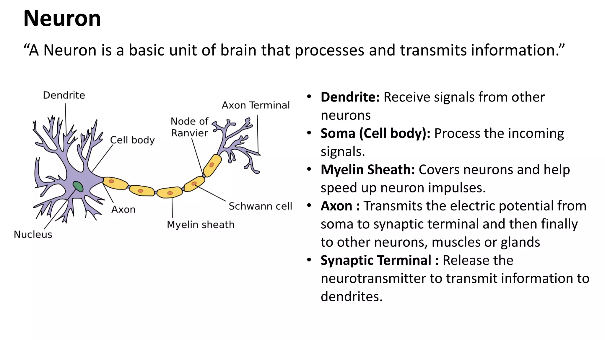
“A Neuron isa basic unit of brain that processes and transmits information.” Neuron • Dendrite: Receive signals from other neurons • Soma (Cell body): Process the incoming signals. • Myelin Sheath: Covers neurons and help speed up neuron impulses. • Axon : Transmits the electric potential from soma to synaptic terminal and then finally to other neurons, muscles or glands • Synaptic Terminal : Release the neurotransmitter to transmit information to dendrites.
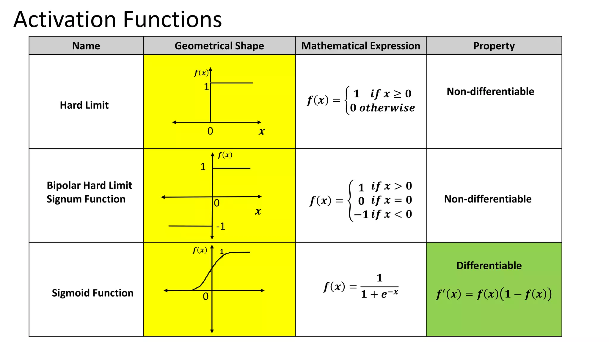
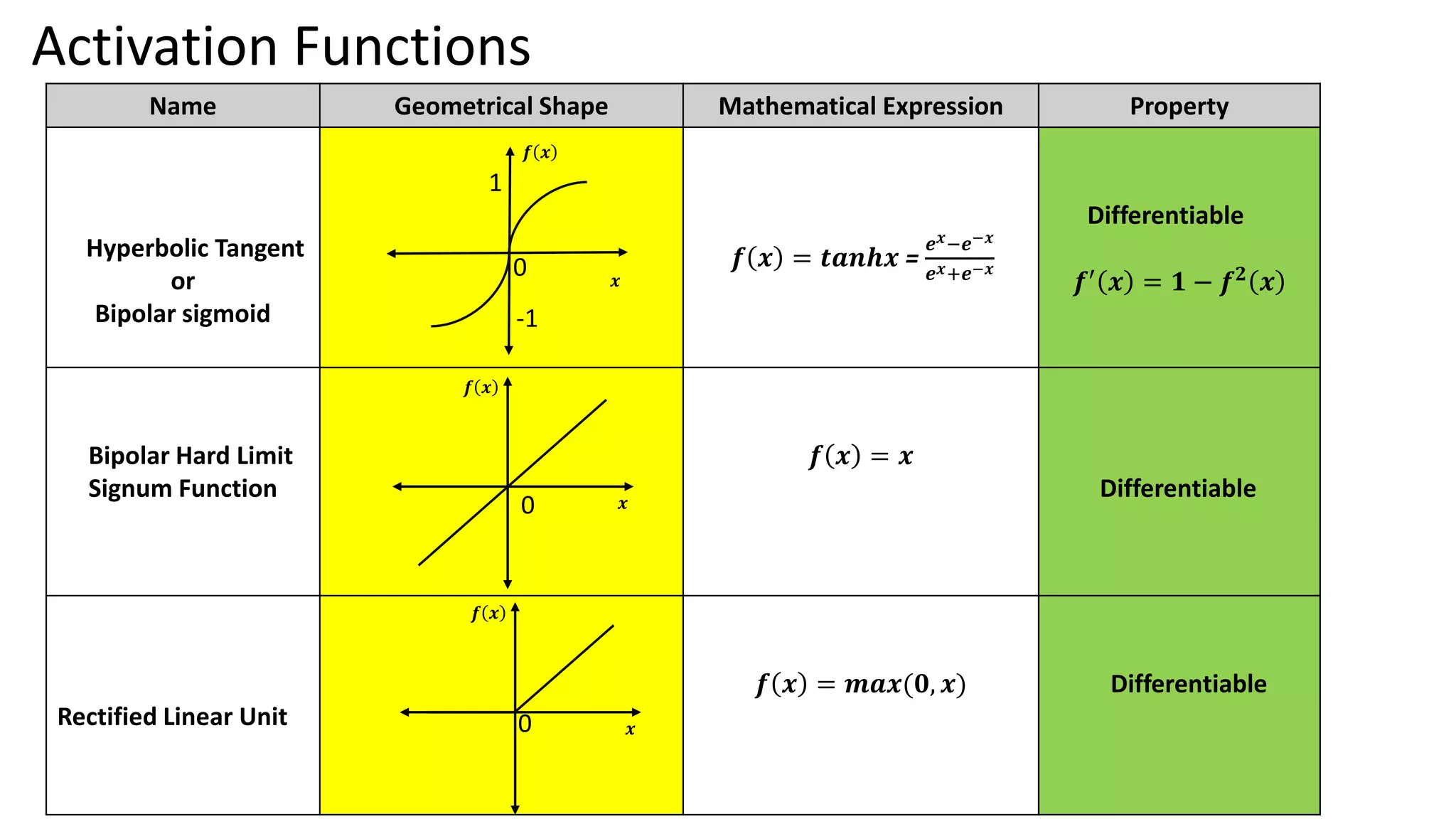
Activation Functions Name GeometricalShape Mathematical Expression Property Hyperbolic Tangent or Bipolar sigmoid 𝒇 𝒙 = 𝒕𝒂𝒏𝒉𝒙 = 𝒆𝒙−𝒆−𝒙 𝒆𝒙+𝒆−𝒙 Differentiable 𝒇′ 𝒙 = 𝟏 − 𝒇𝟐 𝒙 Bipolar Hard Limit Signum Function 𝒇 𝒙 = 𝒙 Differentiable Rectified Linear Unit 𝒇 𝒙 = 𝒎𝒂𝒙(𝟎, 𝒙) Differentiable 0 1 0 𝒙 𝒇 𝒙 -1 𝒇 𝒙 𝒙 𝒇 𝒙 𝒙 0
24.
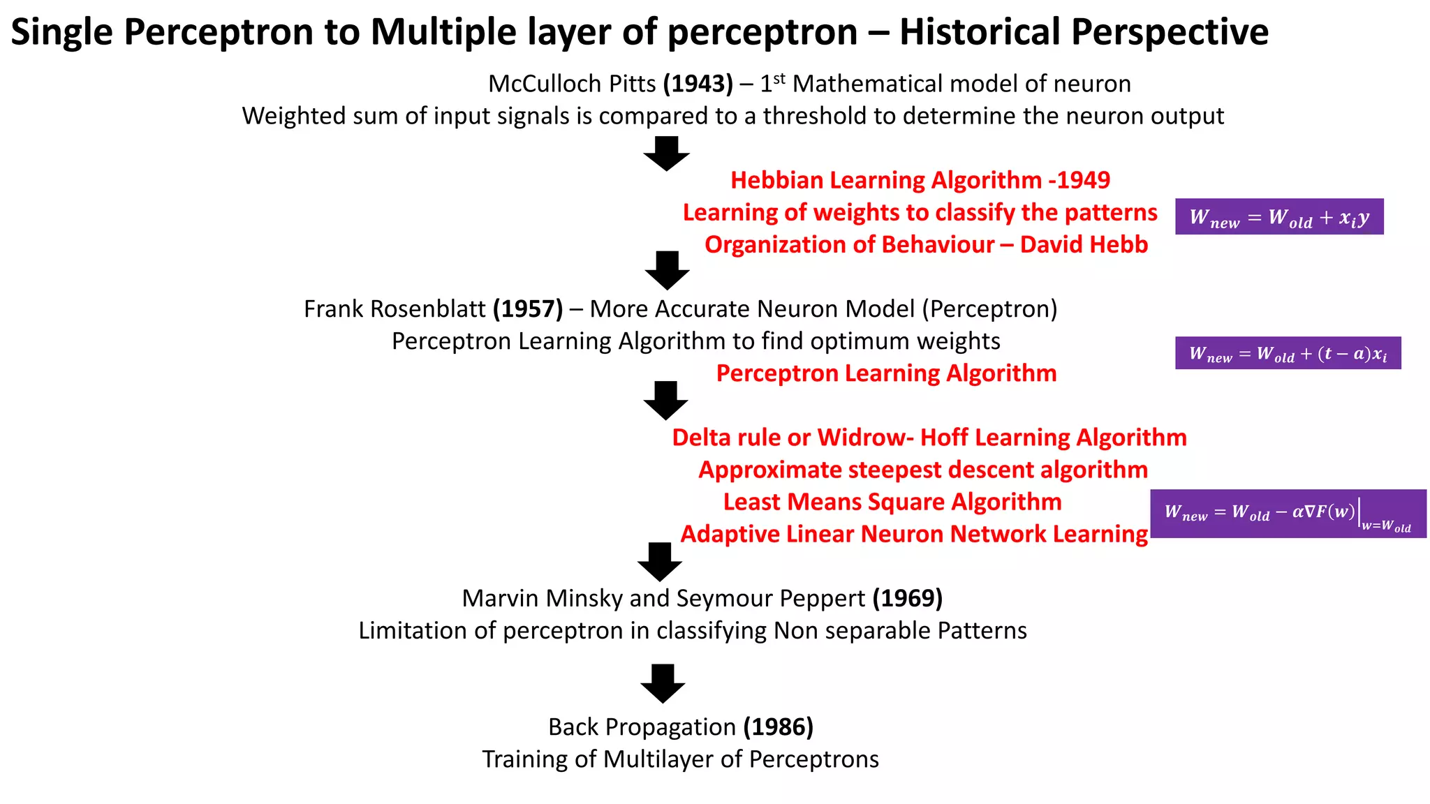
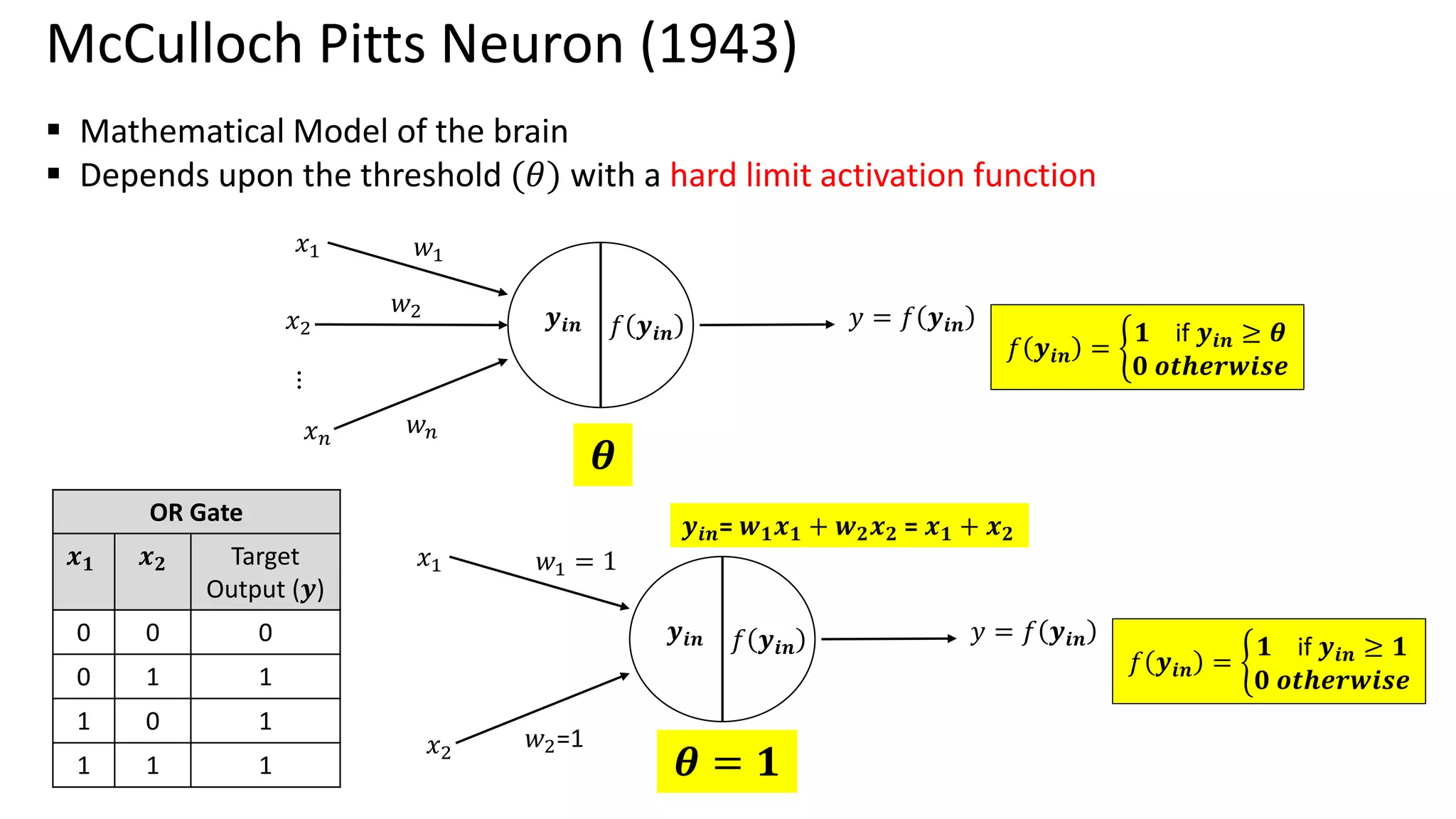
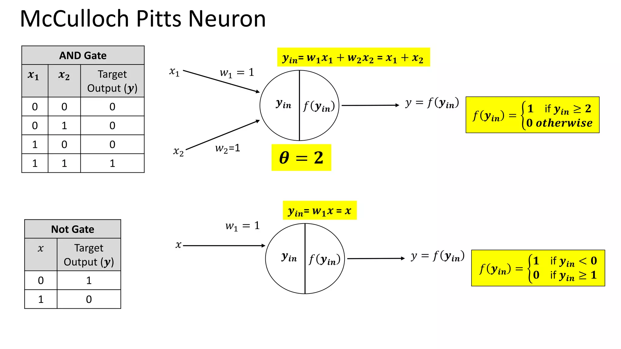
Single Perceptron toMultiple layer of perceptron – Historical Perspective McCulloch Pitts (1943) – 1st Mathematical model of neuron Weighted sum of input signals is compared to a threshold to determine the neuron output Hebbian Learning Algorithm -1949 Learning of weights to classify the patterns Organization of Behaviour – David Hebb Frank Rosenblatt (1957) – More Accurate Neuron Model (Perceptron) Perceptron Learning Algorithm to find optimum weights Perceptron Learning Algorithm Delta rule or Widrow- Hoff Learning Algorithm Approximate steepest descent algorithm Least Means Square Algorithm Adaptive Linear Neuron Network Learning Marvin Minsky and Seymour Peppert (1969) Limitation of perceptron in classifying Non separable Patterns Back Propagation (1986) Training of Multilayer of Perceptrons 𝑾𝒏𝒆𝒘 = 𝑾𝒐𝒍𝒅 + 𝒙𝒊𝒚 𝑾𝒏𝒆𝒘 = 𝑾𝒐𝒍𝒅 + (𝒕 − 𝒂)𝒙𝒊 𝑾𝒏𝒆𝒘 = 𝑾𝒐𝒍𝒅 − ቚ 𝜶𝛁𝑭 𝒘 𝒘=𝑾𝒐𝒍𝒅
25.
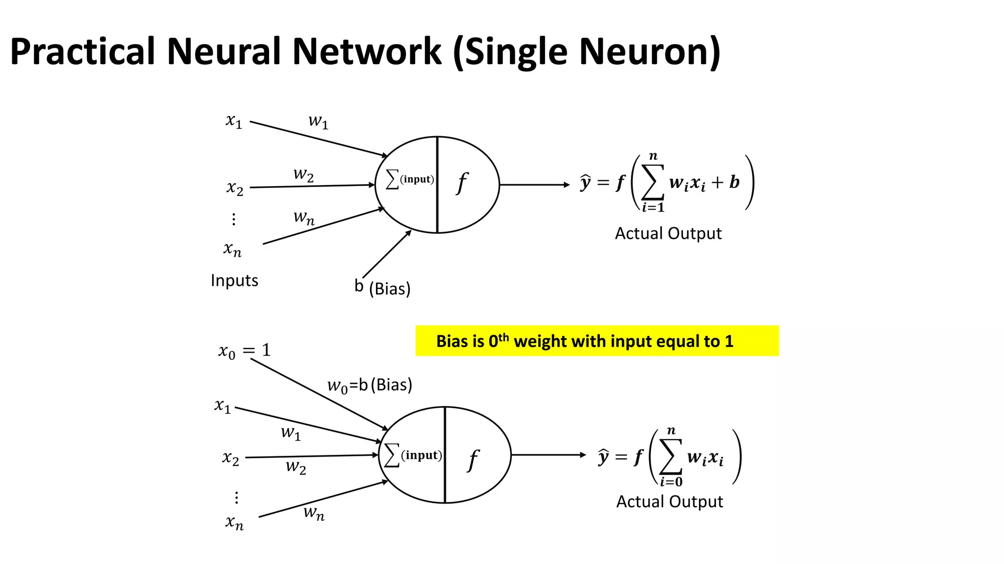
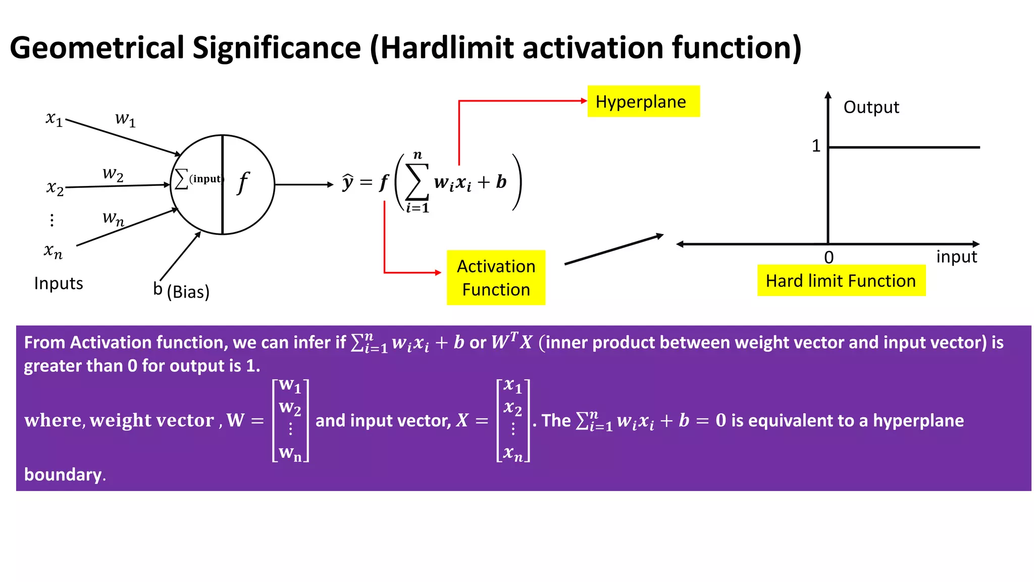
Geometrical Significance (Hardlimitactivation function) 𝑥1 𝑥2 𝑥𝑛 ⋮ 𝑤1 𝑤2 𝑤𝑛 ෝ 𝒚 = 𝒇 𝒊=𝟏 𝒏 𝒘𝒊𝒙𝒊 + 𝒃 (𝐢𝐧𝐩𝐮𝐭) 𝑓 Inputs b (Bias) Hyperplane Activation Function 0 1 Output input Hard limit Function From Activation function, we can infer if σ𝒊=𝟏 𝒏 𝒘𝒊𝒙𝒊 + 𝒃 or 𝑾𝑻 𝑿 (inner product between weight vector and input vector) is greater than 0 for output is 1. 𝐰𝐡𝐞𝐫𝐞, 𝐰𝐞𝐢𝐠𝐡𝐭 𝐯𝐞𝐜𝐭𝐨𝐫 , 𝐖 = 𝐰𝟏 𝐰𝟐 ⋮ 𝐰𝐧 and input vector, 𝑿 = 𝒙𝟏 𝒙𝟐 ⋮ 𝒙𝒏 . The σ𝒊=𝟏 𝒏 𝒘𝒊𝒙𝒊 + 𝒃 = 𝟎 is equivalent to a hyperplane boundary.
26.
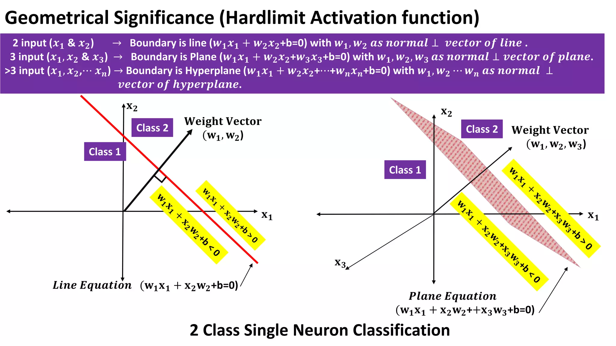
Geometrical Significance (HardlimitActivation function) 2 input (𝒙𝟏 & 𝒙𝟐) → Boundary is line (𝒘𝟏𝒙𝟏 + 𝒘𝟐𝒙𝟐+b=0) with 𝒘𝟏, 𝒘𝟐 𝒂𝒔 𝒏𝒐𝒓𝒎𝒂𝒍 ⊥ 𝒗𝒆𝒄𝒕𝒐𝒓 𝒐𝒇 𝒍𝒊𝒏𝒆 . 3 input (𝒙𝟏, 𝒙𝟐 & 𝒙𝟑) → Boundary is Plane (𝒘𝟏𝒙𝟏 + 𝒘𝟐𝒙𝟐+𝒘𝟑𝒙𝟑+b=0) with 𝒘𝟏, 𝒘𝟐, 𝒘𝟑 𝒂𝒔 𝒏𝒐𝒓𝒎𝒂𝒍 ⊥ 𝒗𝒆𝒄𝒕𝒐𝒓 𝒐𝒇 𝒑𝒍𝒂𝒏𝒆. >3 input (𝒙𝟏, 𝒙𝟐,⋯ 𝒙𝒏) → Boundary is Hyperplane (𝒘𝟏𝒙𝟏 + 𝒘𝟐𝒙𝟐+⋯+𝒘𝒏𝒙𝒏+b=0) with 𝒘𝟏, 𝒘𝟐 ⋯ 𝒘𝒏 𝒂𝒔 𝒏𝒐𝒓𝒎𝒂𝒍 ⊥ 𝒗𝒆𝒄𝒕𝒐𝒓 𝒐𝒇 𝒉𝒚𝒑𝒆𝒓𝒑𝒍𝒂𝒏𝒆. 𝐖𝐞𝐢𝐠𝐡𝐭 𝐕𝐞𝐜𝐭𝐨𝐫 (𝐰𝟏, 𝐰𝟐) 𝑳𝒊𝒏𝒆 𝑬𝒒𝒖𝒂𝒕𝒊𝒐𝒏 (𝐰𝟏𝐱𝟏 + 𝐱𝟐𝐰𝟐+b=0) Class 1 Class 2 𝐖𝐞𝐢𝐠𝐡𝐭 𝐕𝐞𝐜𝐭𝐨𝐫 (𝐰𝟏, 𝐰𝟐, 𝐰𝟑) 𝑷𝒍𝒂𝒏𝒆 𝑬𝒒𝒖𝒂𝒕𝒊𝒐𝒏 (𝐰𝟏𝐱𝟏 + 𝐱𝟐𝐰𝟐++𝐱𝟑𝐰𝟑+b=0) Class 1 Class 2 𝐱𝟏 𝐱𝟐 𝐱𝟏 𝐱𝟐 𝐱𝟑 2 Class Single Neuron Classification
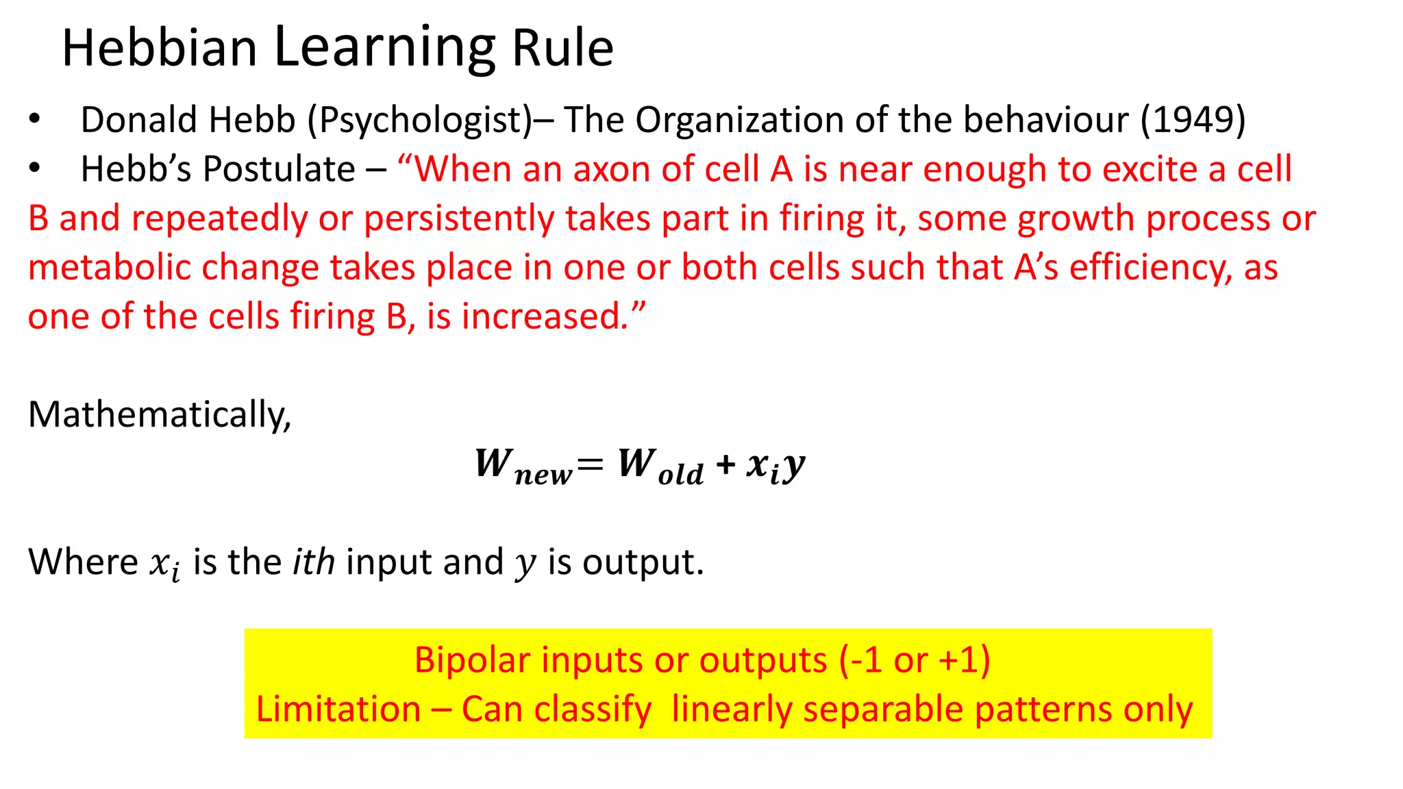
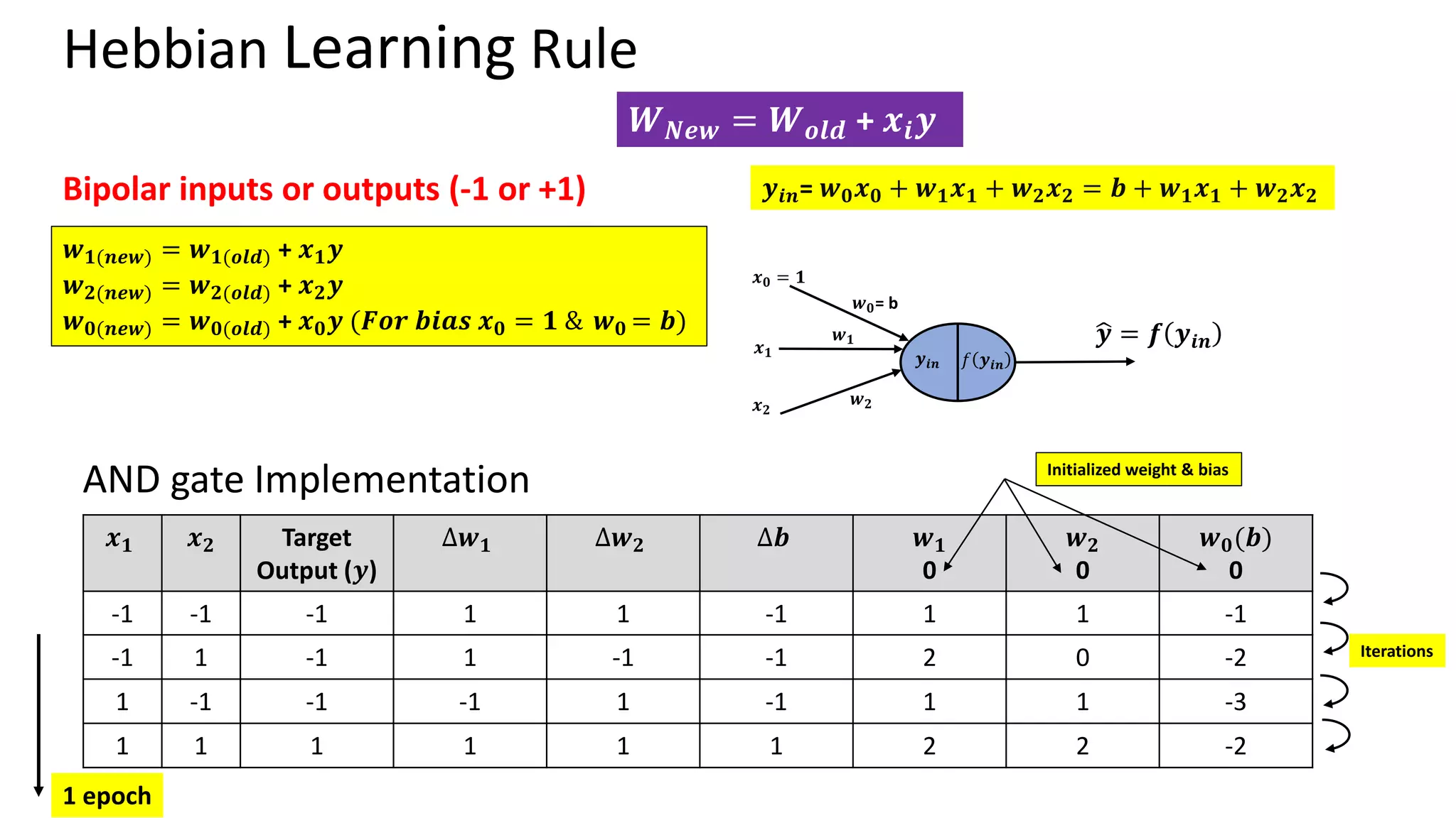
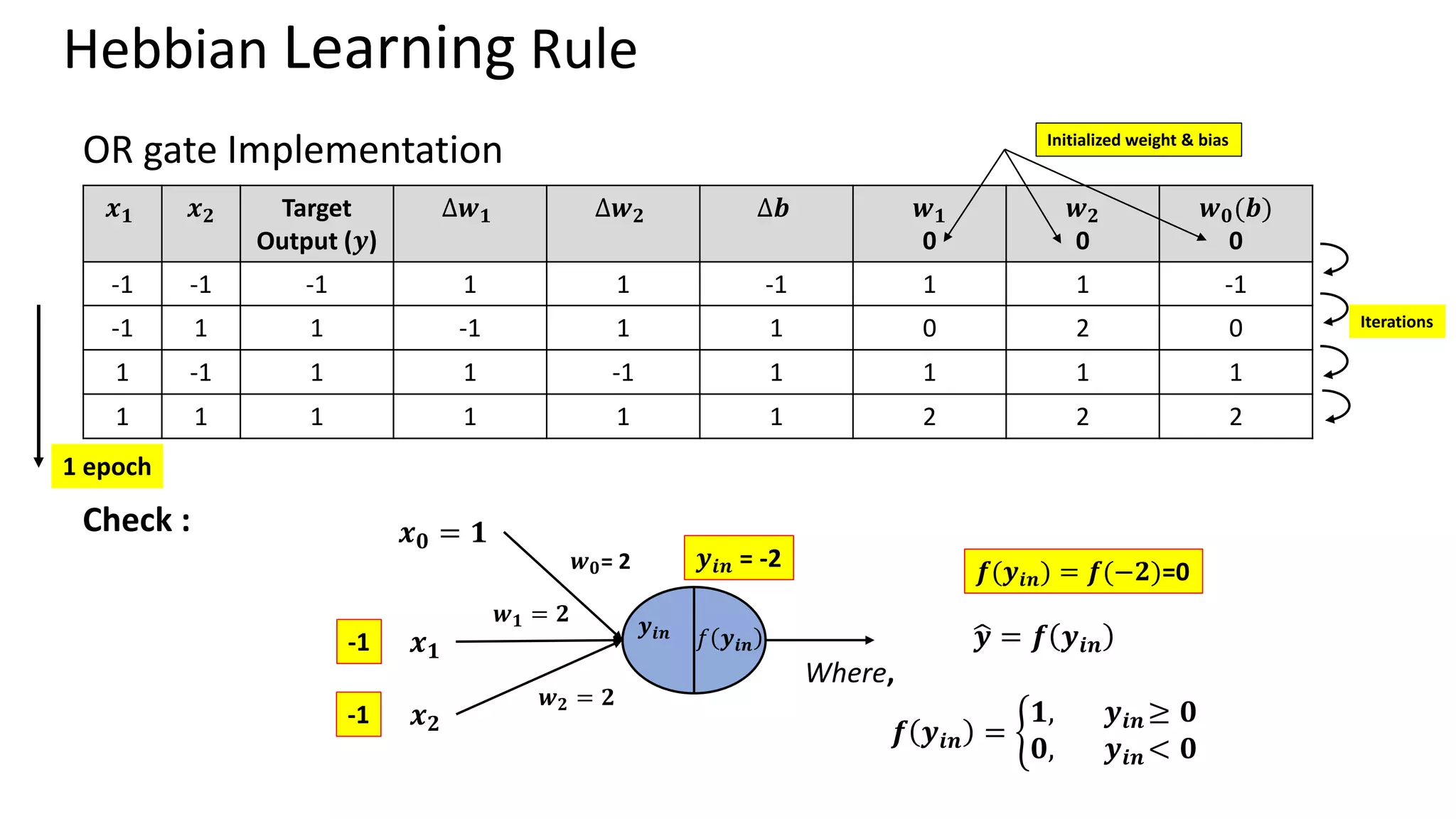
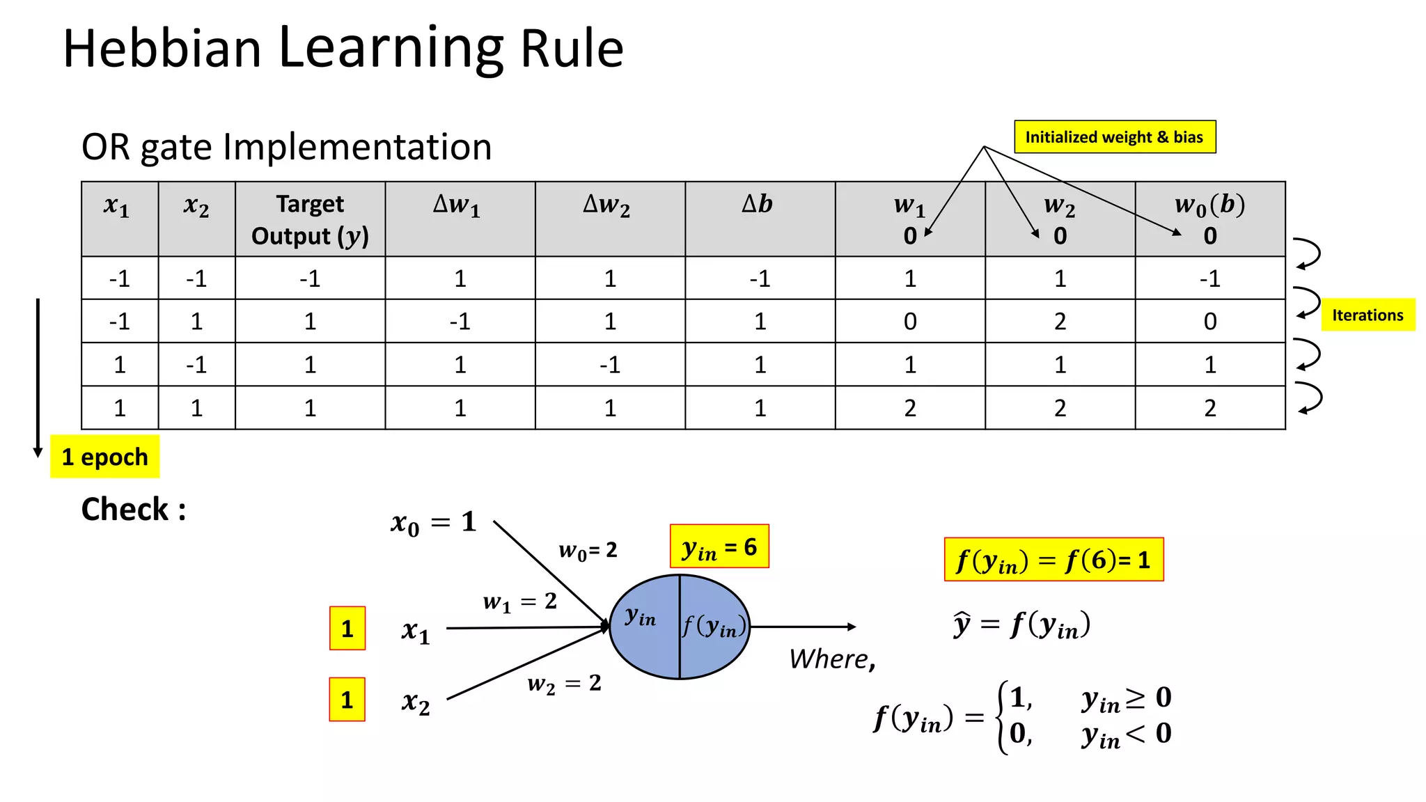
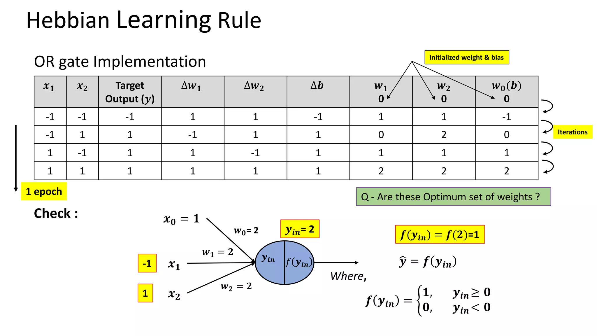
Hebbian Learning Rule •Donald Hebb (Psychologist)– The Organization of the behaviour (1949) • Hebb’s Postulate – “When an axon of cell A is near enough to excite a cell B and repeatedly or persistently takes part in firing it, some growth process or metabolic change takes place in one or both cells such that A’s efficiency, as one of the cells firing B, is increased.” Mathematically, 𝑾𝒏𝒆𝒘= 𝑾𝒐𝒍𝒅 + 𝒙𝒊𝒚 Where 𝑥𝑖 is the ith input and 𝑦 is output. Bipolar inputs or outputs (-1 or +1) Limitation – Can classify linearly separable patterns only
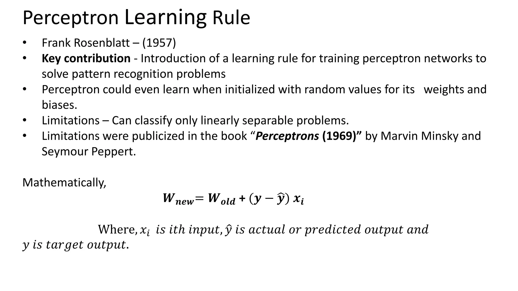
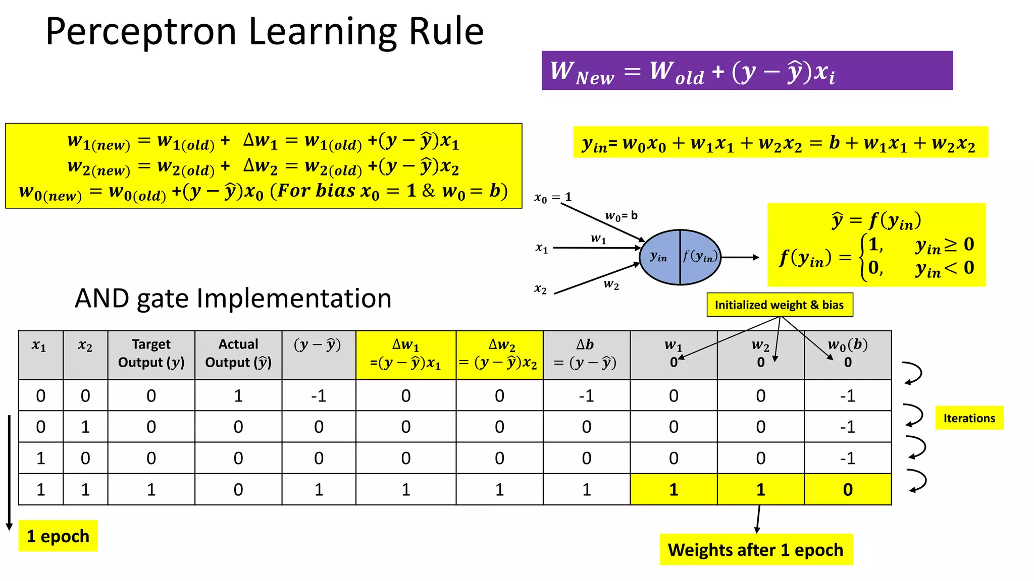
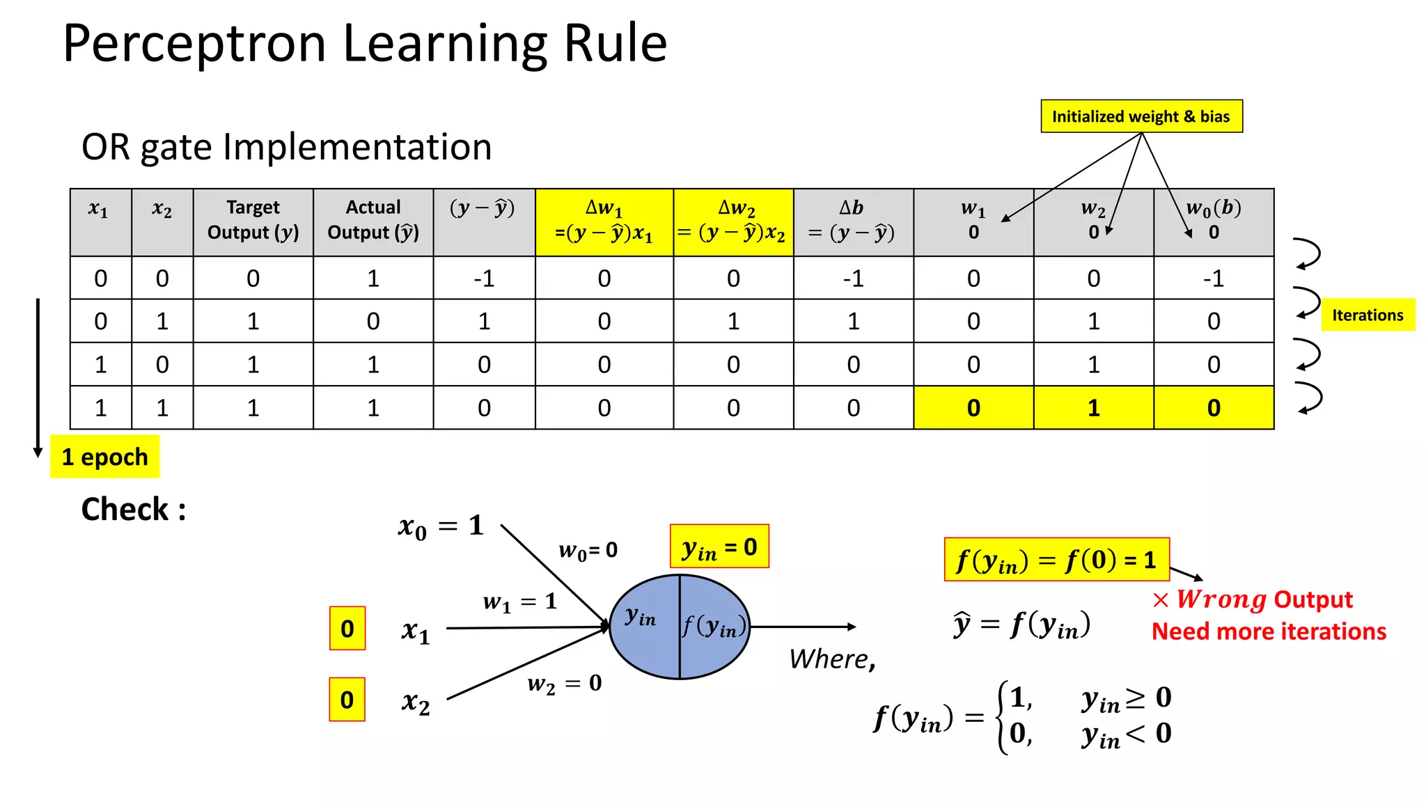
Perceptron Learning Rule •Frank Rosenblatt – (1957) • Key contribution - Introduction of a learning rule for training perceptron networks to solve pattern recognition problems • Perceptron could even learn when initialized with random values for its weights and biases. • Limitations – Can classify only linearly separable problems. • Limitations were publicized in the book “Perceptrons (1969)” by Marvin Minsky and Seymour Peppert. Mathematically, 𝑾𝒏𝒆𝒘= 𝑾𝒐𝒍𝒅 + (𝒚 − ෝ 𝒚) 𝒙𝒊 Where, 𝑥𝑖 𝑖𝑠 𝑖𝑡ℎ 𝑖𝑛𝑝𝑢𝑡, ො 𝑦 𝑖𝑠 𝑎𝑐𝑡𝑢𝑎𝑙 𝑜𝑟 𝑝𝑟𝑒𝑑𝑖𝑐𝑡𝑒𝑑 𝑜𝑢𝑡𝑝𝑢𝑡 𝑎𝑛𝑑 𝑦 𝑖𝑠 𝑡𝑎𝑟𝑔𝑒𝑡 𝑜𝑢𝑡𝑝𝑢𝑡.