Download to read offline


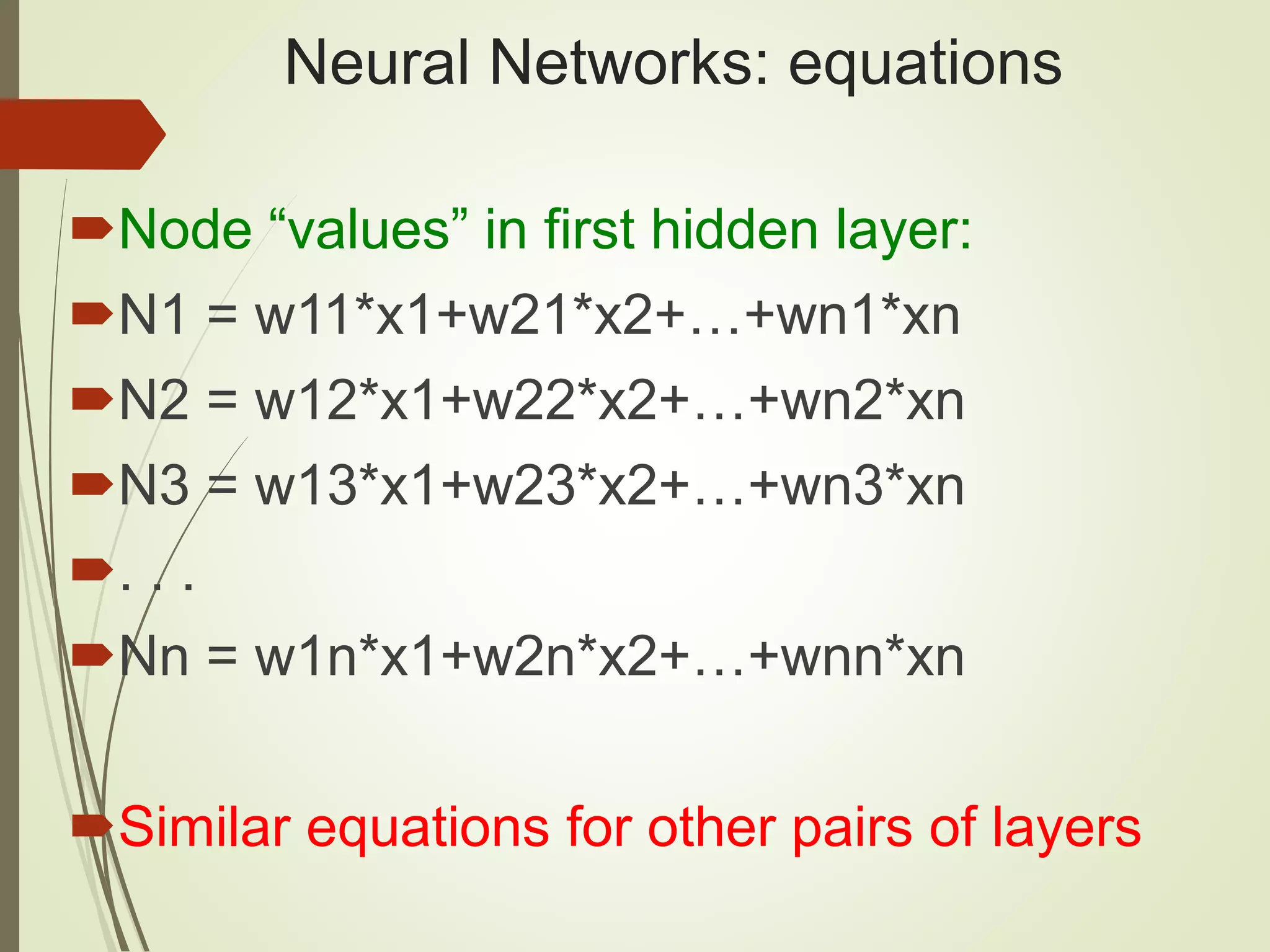

![Setting up Data & the Model Normalize the data: Subtract the ‘mean’ and divide by stddev [Central Limit Theorem] Initial weight values for NNs: Random numbers in N(0,1) More details: http://cs231n.github.io/neural-networks-2/#losses](https://image.slidesharecdn.com/sfjavadl-180119024918/75/Java-and-Deep-Learning-Introduction-47-2048.jpg)

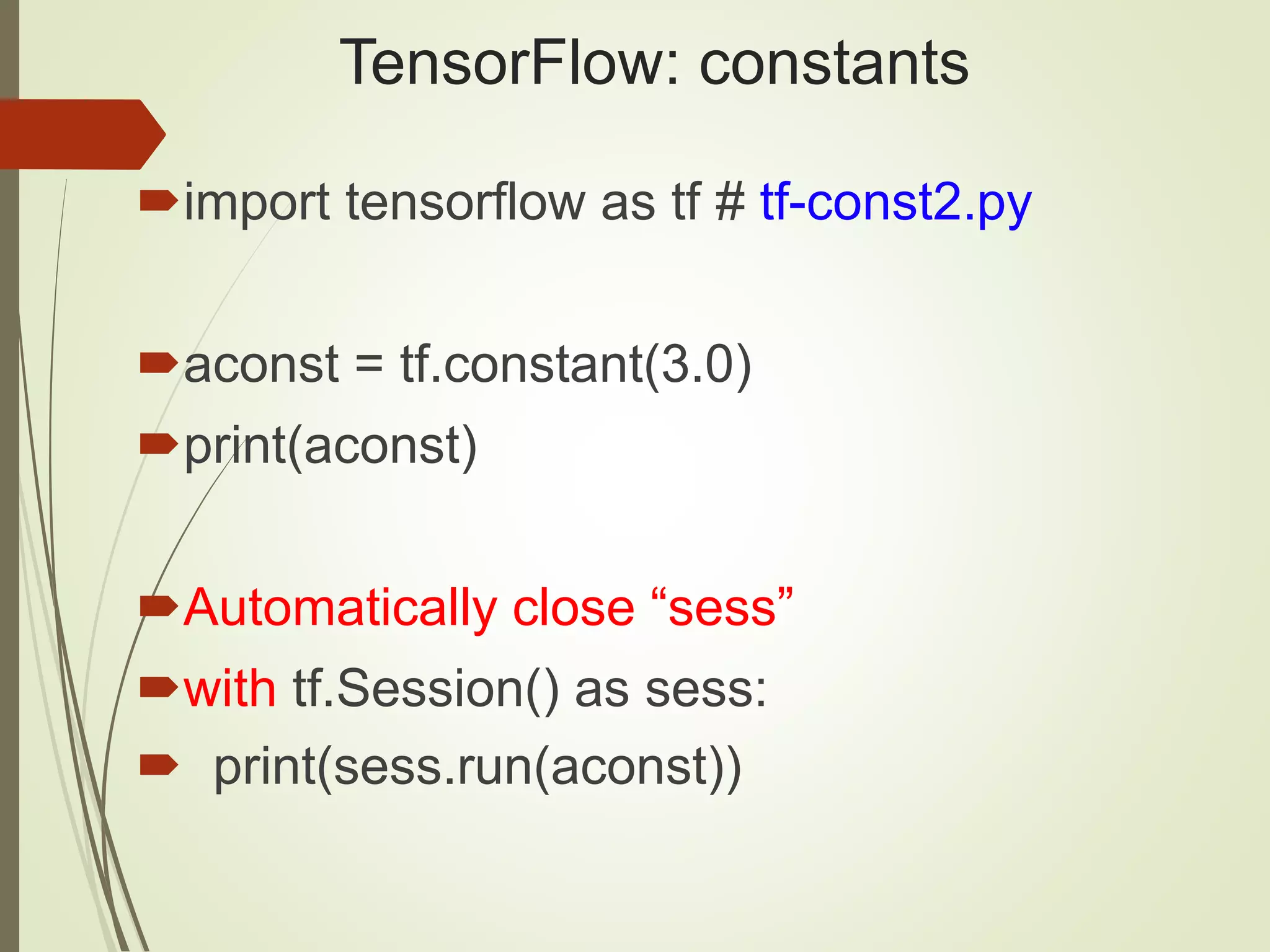
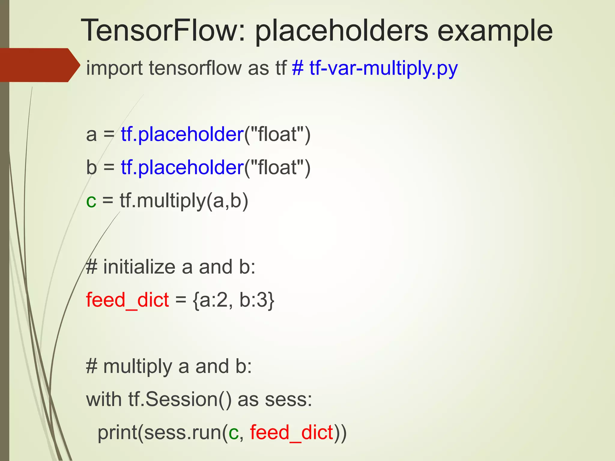
![TensorFlow fetch/feed_dict import tensorflow as tf # fetch-feeddict.py # y = W*x + b: W and x are 1d arrays W = tf.constant([10,20], name=’W’) x = tf.placeholder(tf.int32, name='x') b = tf.placeholder(tf.int32, name='b') Wx = tf.multiply(W, x, name='Wx') y = tf.add(Wx, b, name=’y’)](https://image.slidesharecdn.com/sfjavadl-180119024918/75/Java-and-Deep-Learning-Introduction-84-2048.jpg)
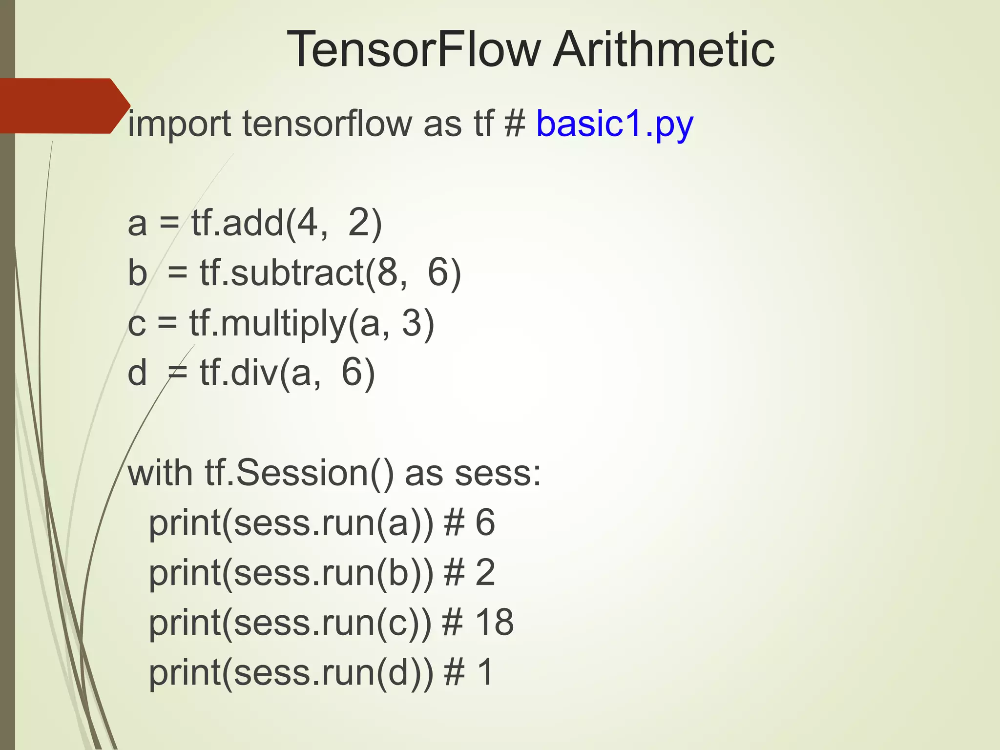
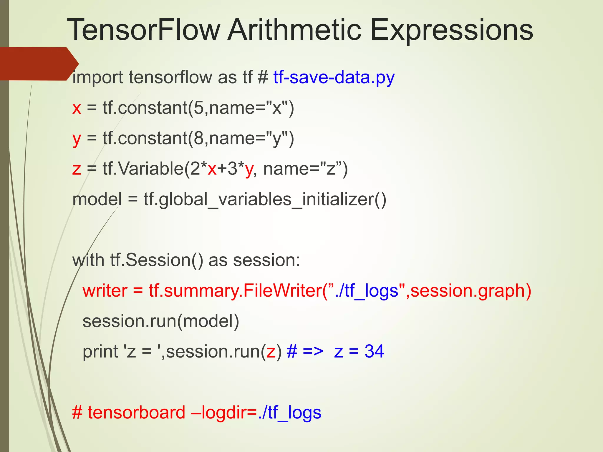
![TensorFlow fetch/feed_dict with tf.Session() as sess: print("Result 1: Wx = ", sess.run(Wx, feed_dict={x:[5,10]})) print("Result 2: y = ", sess.run(y, feed_dict={x:[5,10], b:[15,25]})) Result 1: Wx = [50 200] Result 2: y = [65 225]](https://image.slidesharecdn.com/sfjavadl-180119024918/75/Java-and-Deep-Learning-Introduction-85-2048.jpg)
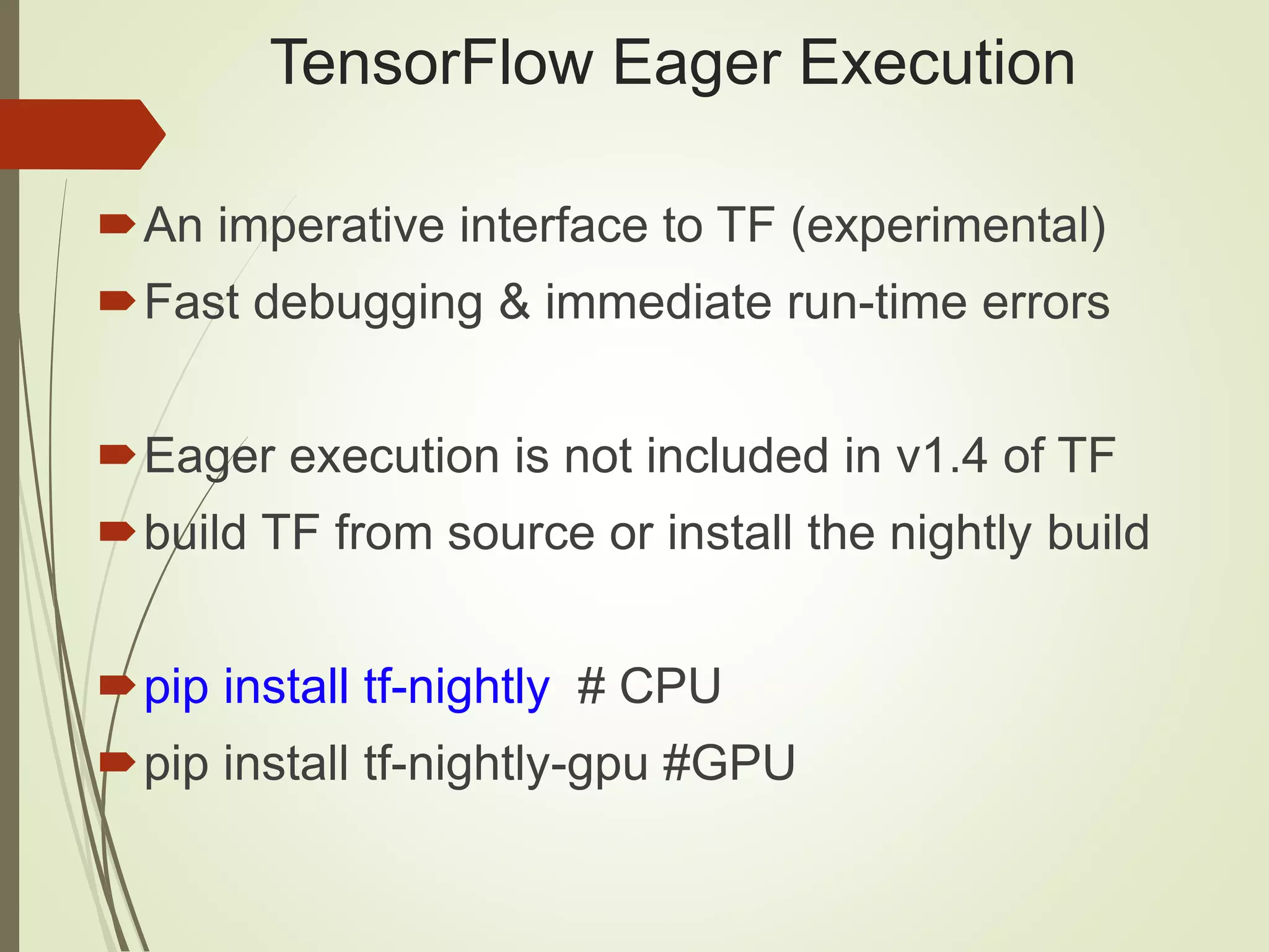
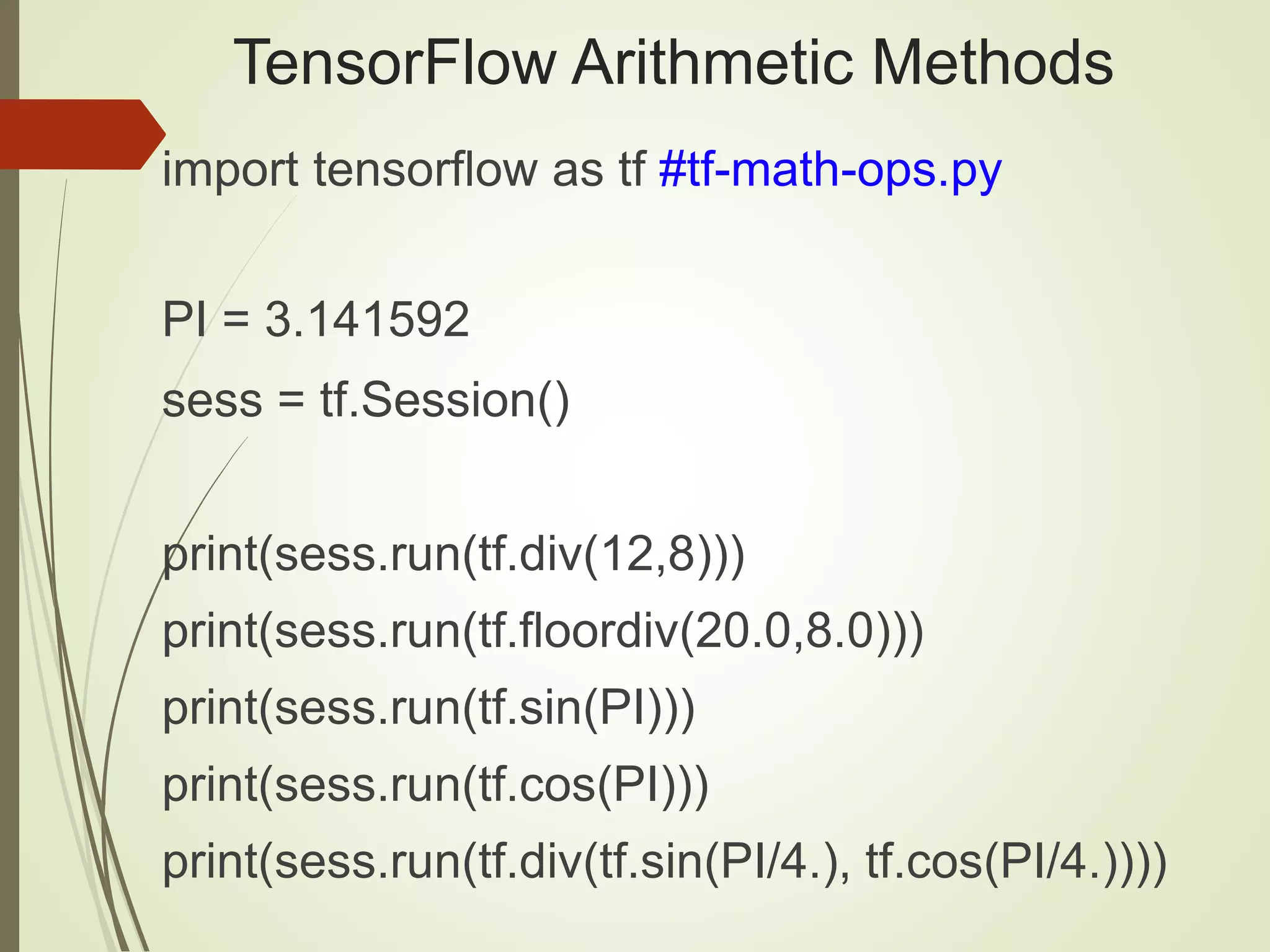
![TensorFlow Eager Execution import tensorflow as tf # tf-eager1.py import tensorflow.contrib.eager as tfe tfe.enable_eager_execution() x = [[2.]] m = tf.matmul(x, x) print(m)](https://image.slidesharecdn.com/sfjavadl-180119024918/75/Java-and-Deep-Learning-Introduction-89-2048.jpg)


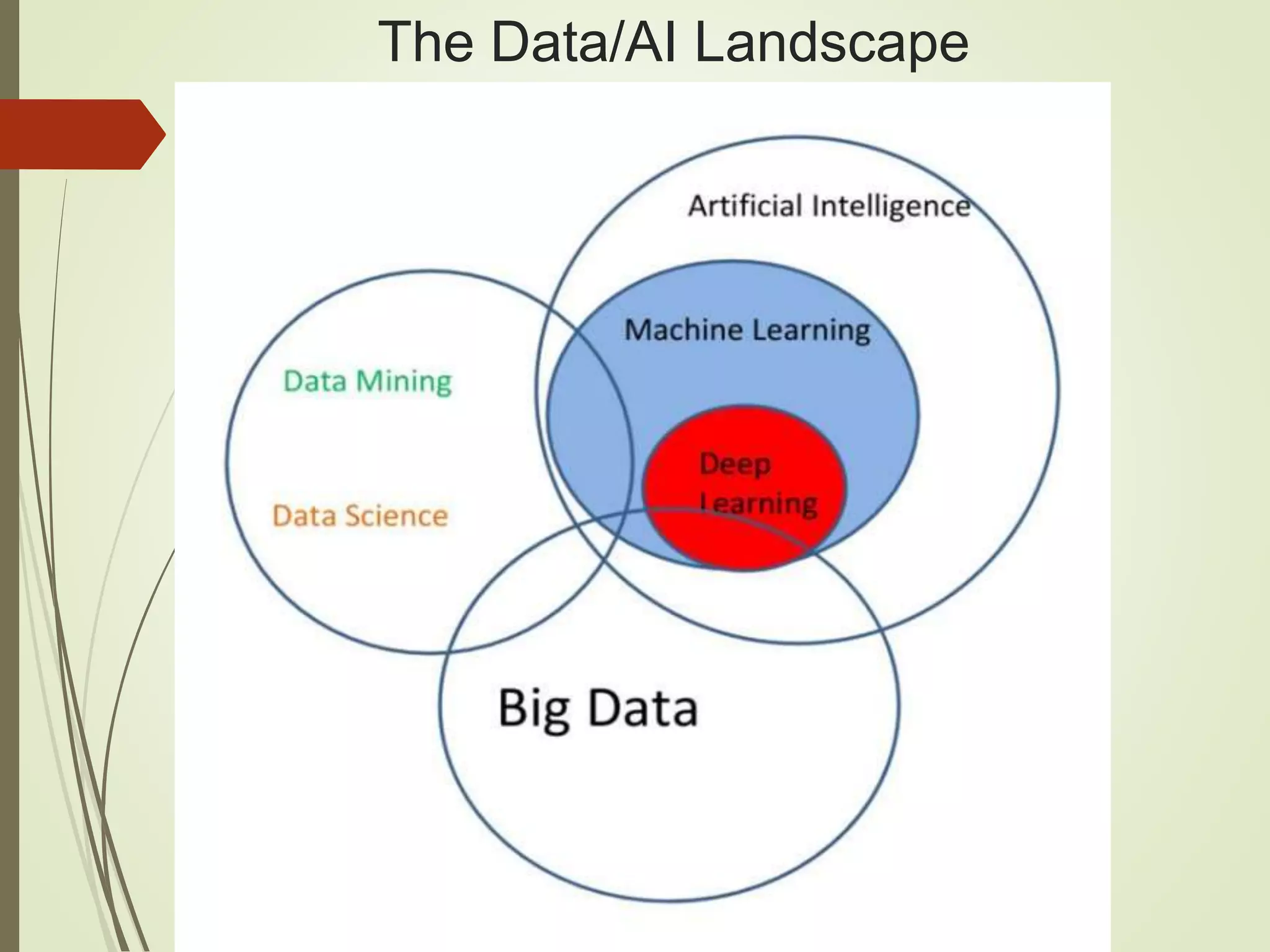
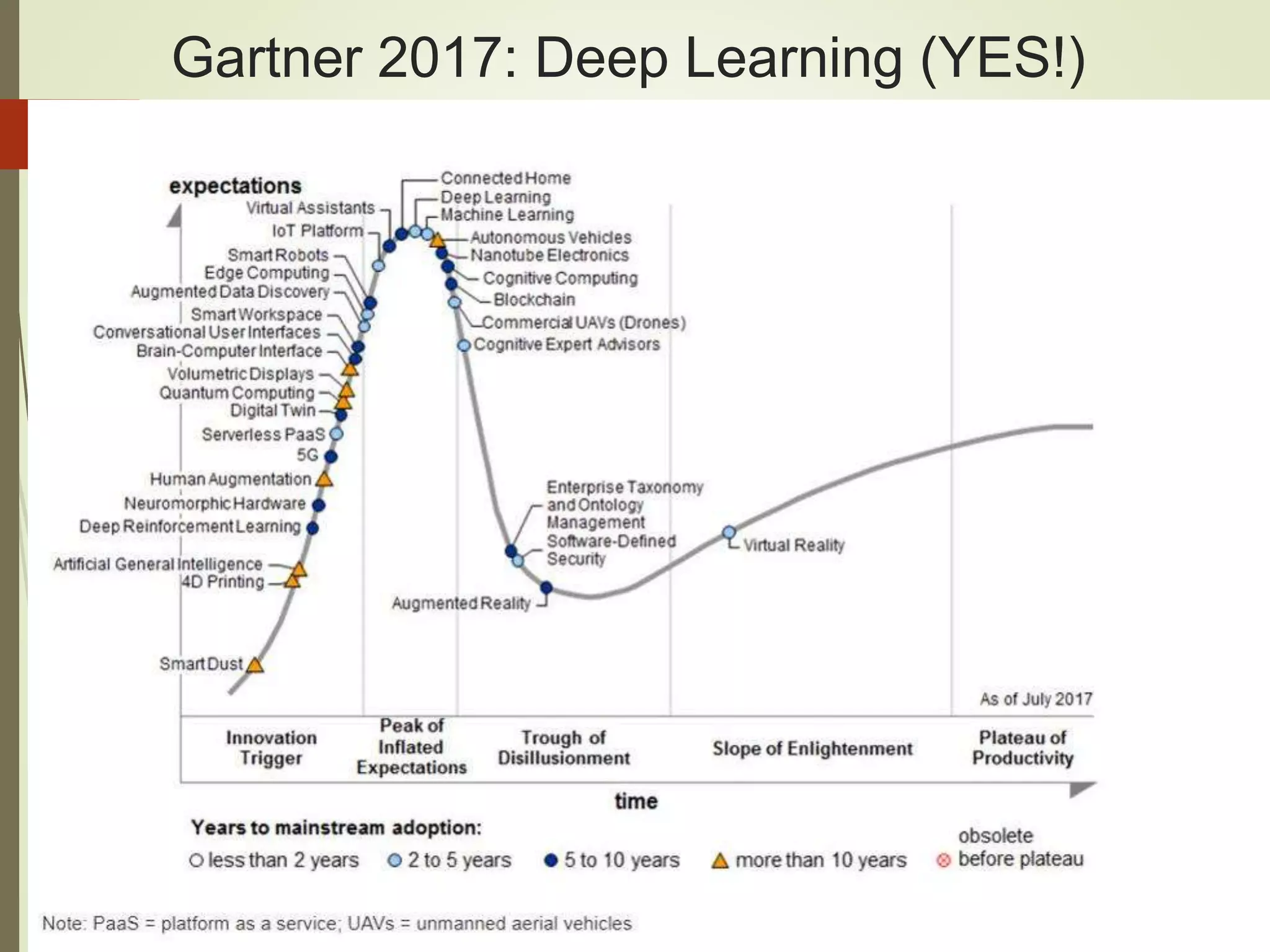
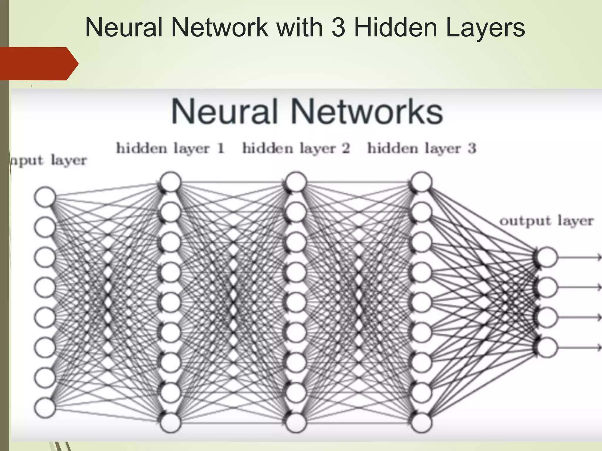
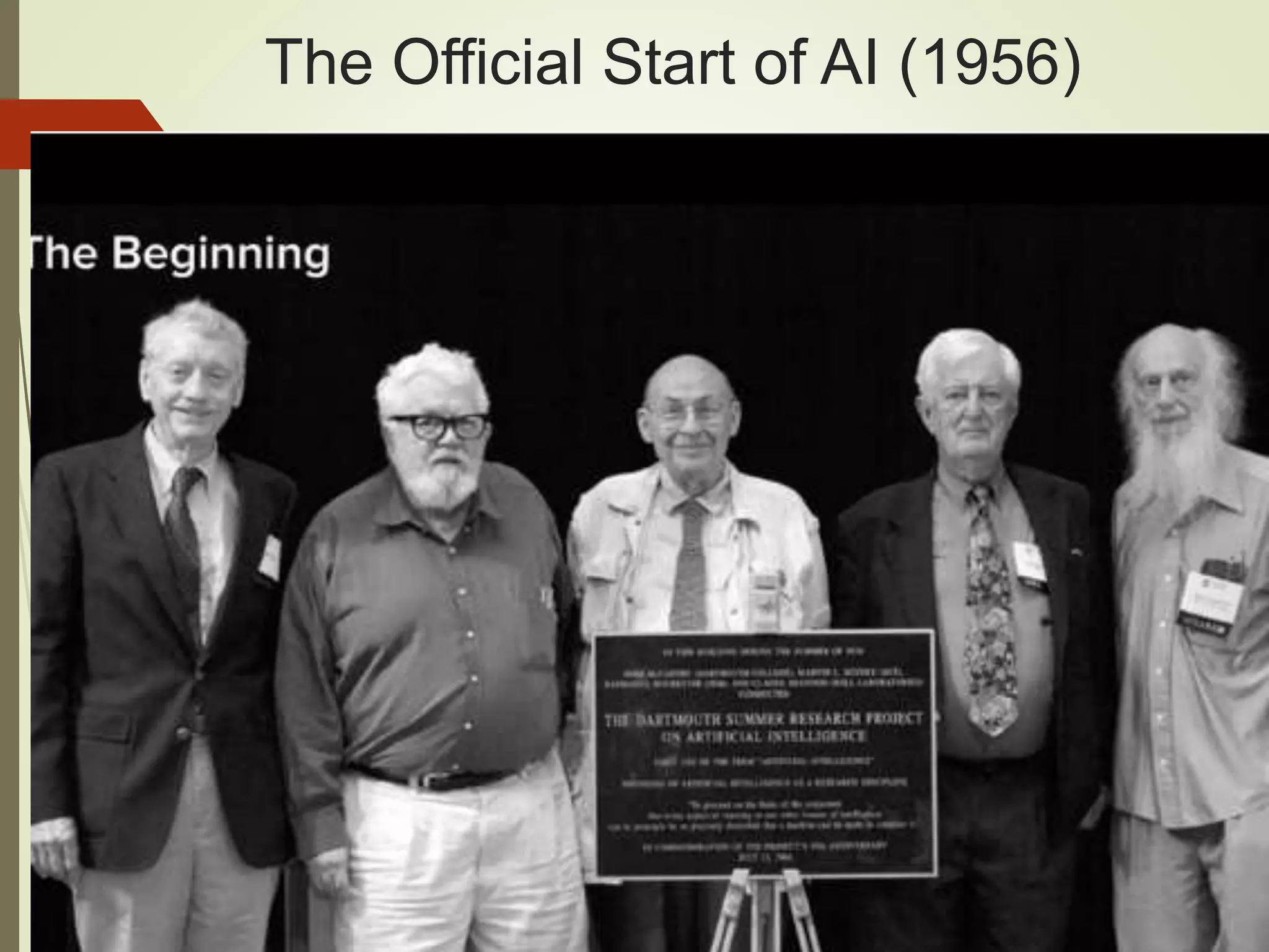
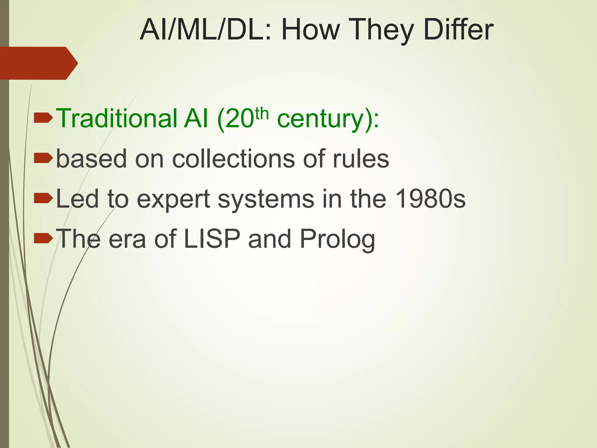
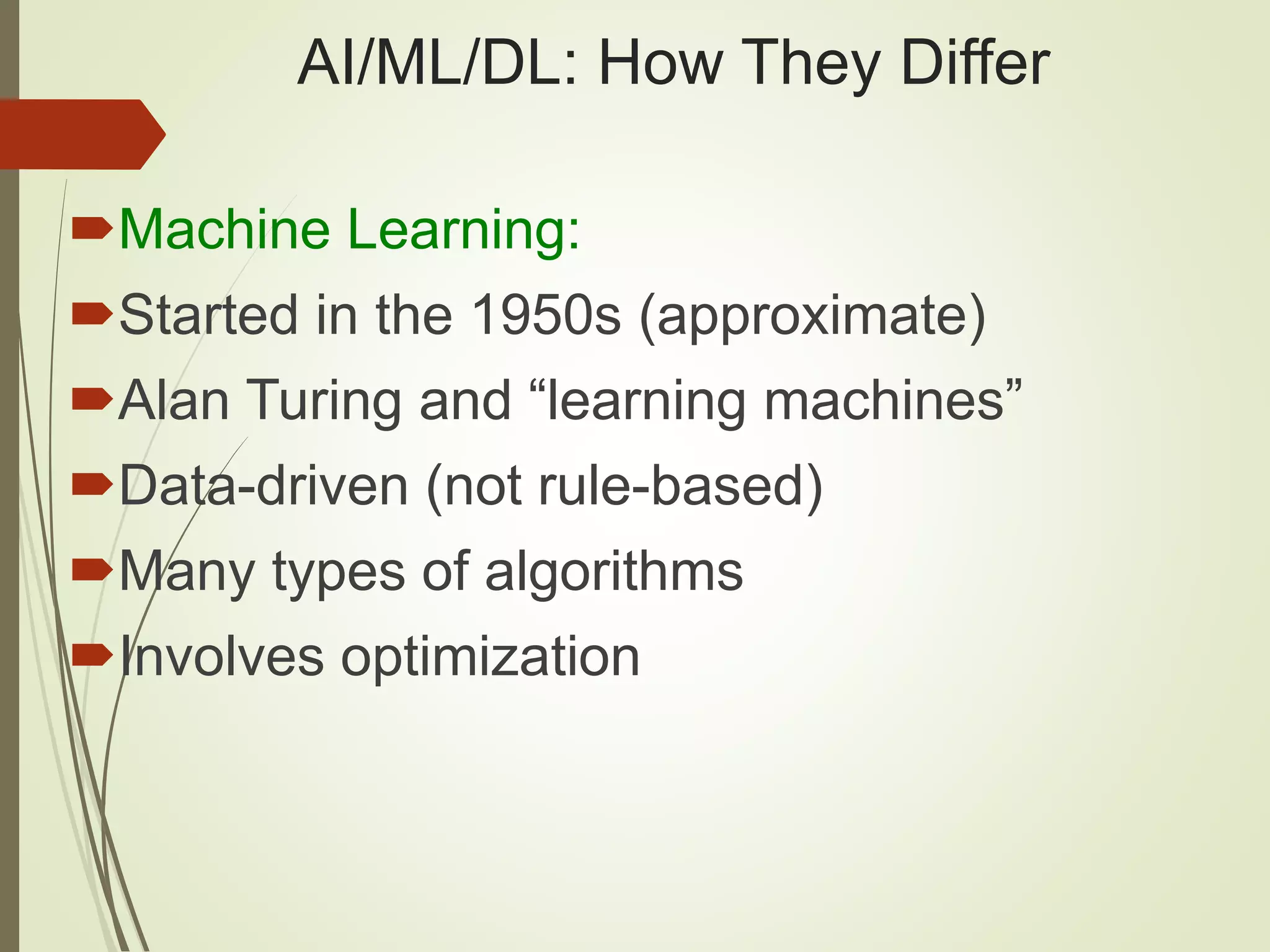
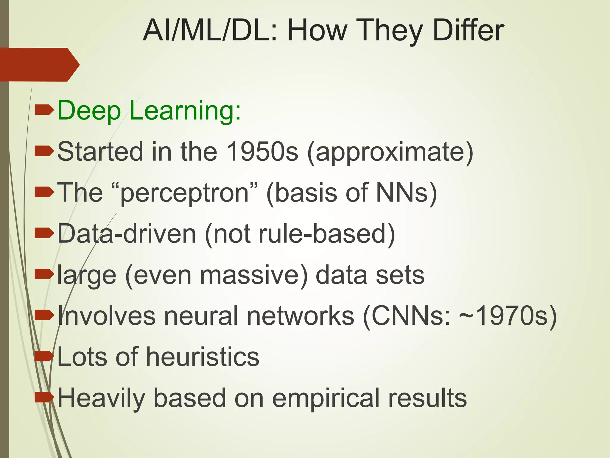
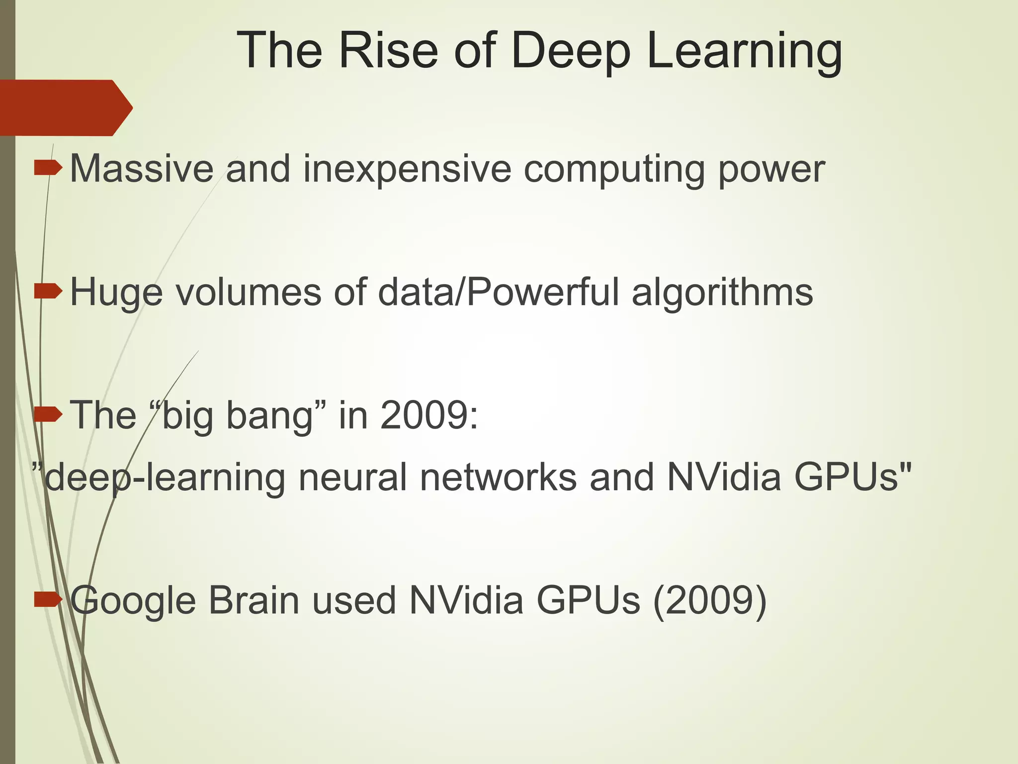
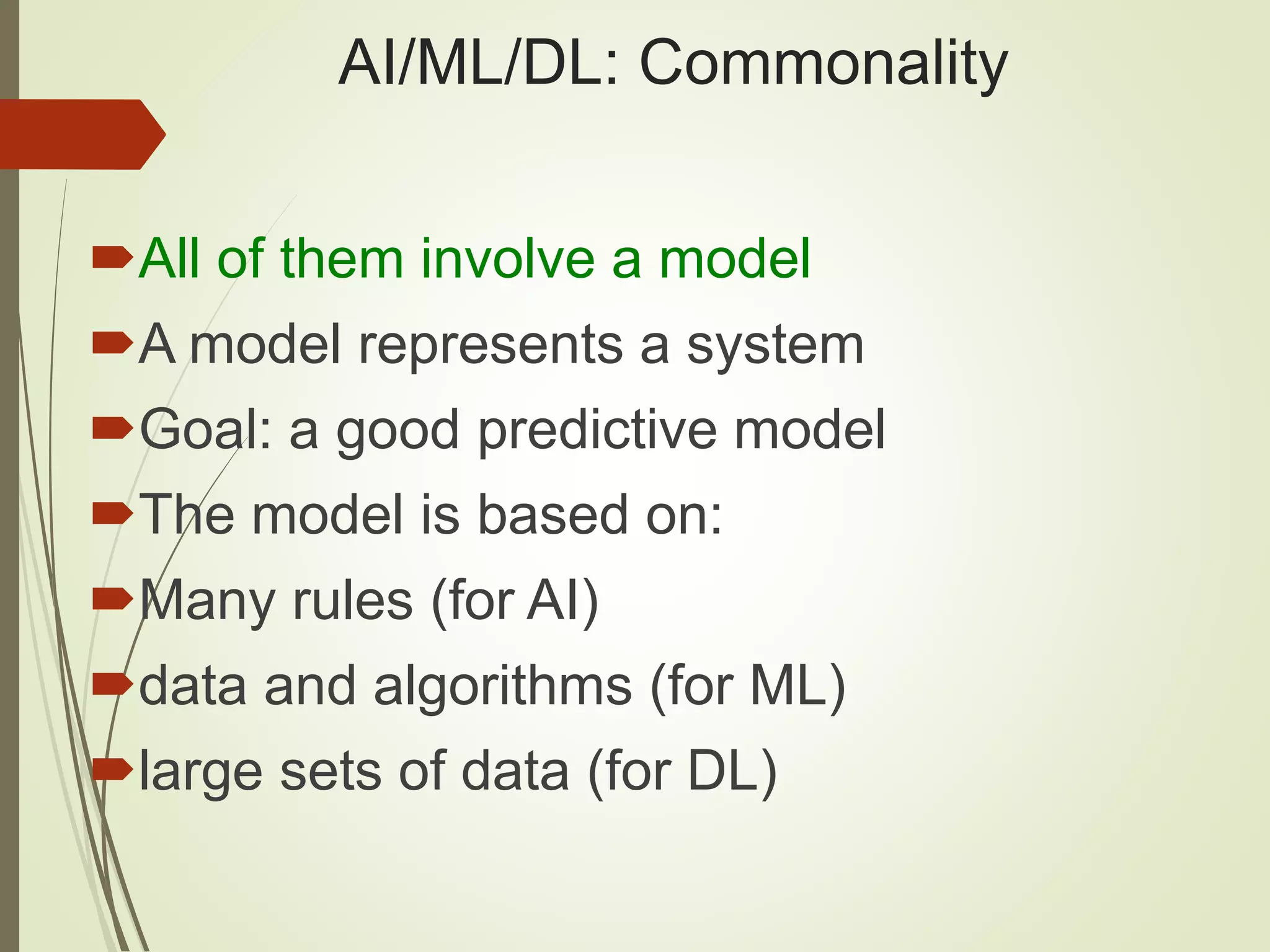
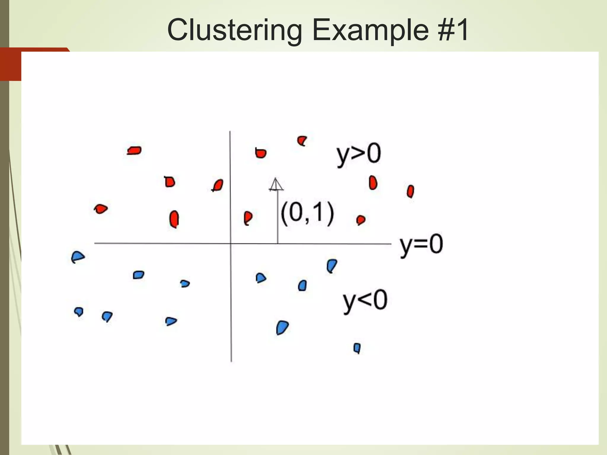
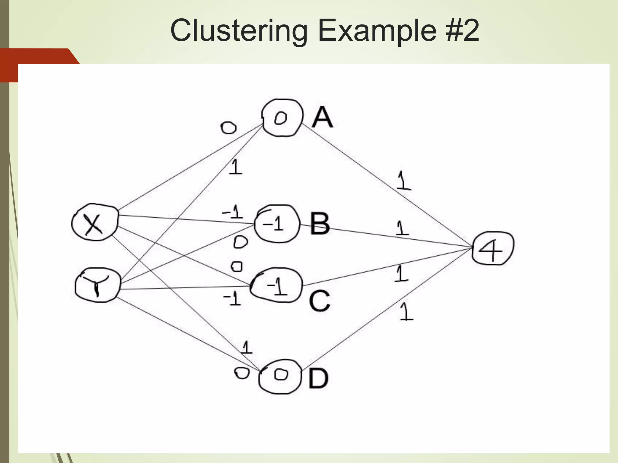
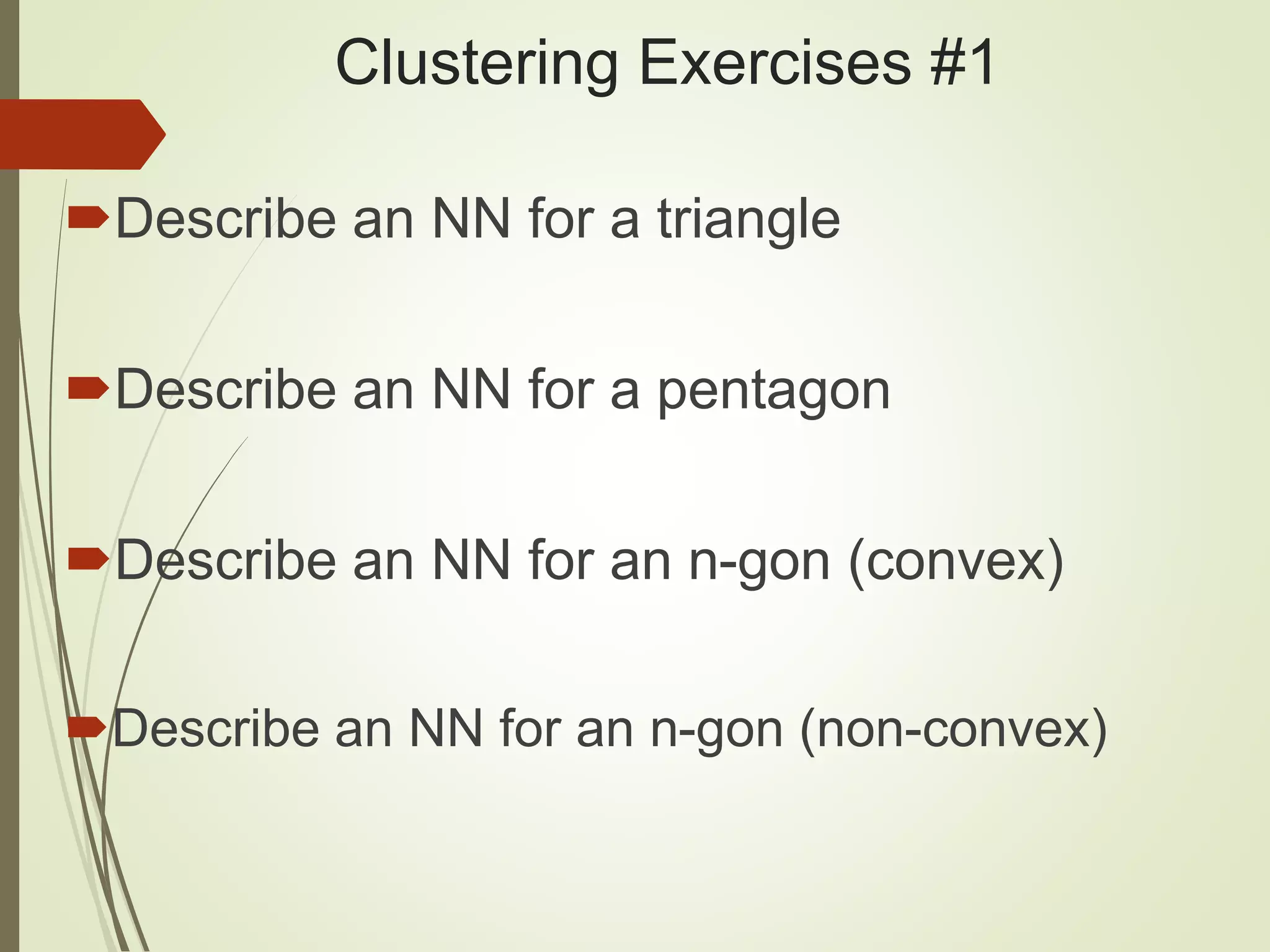
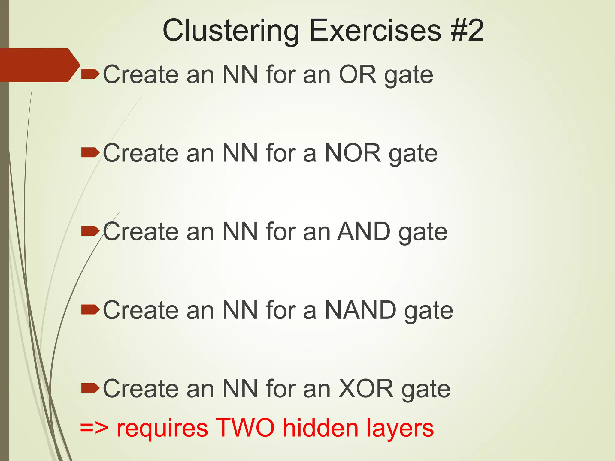
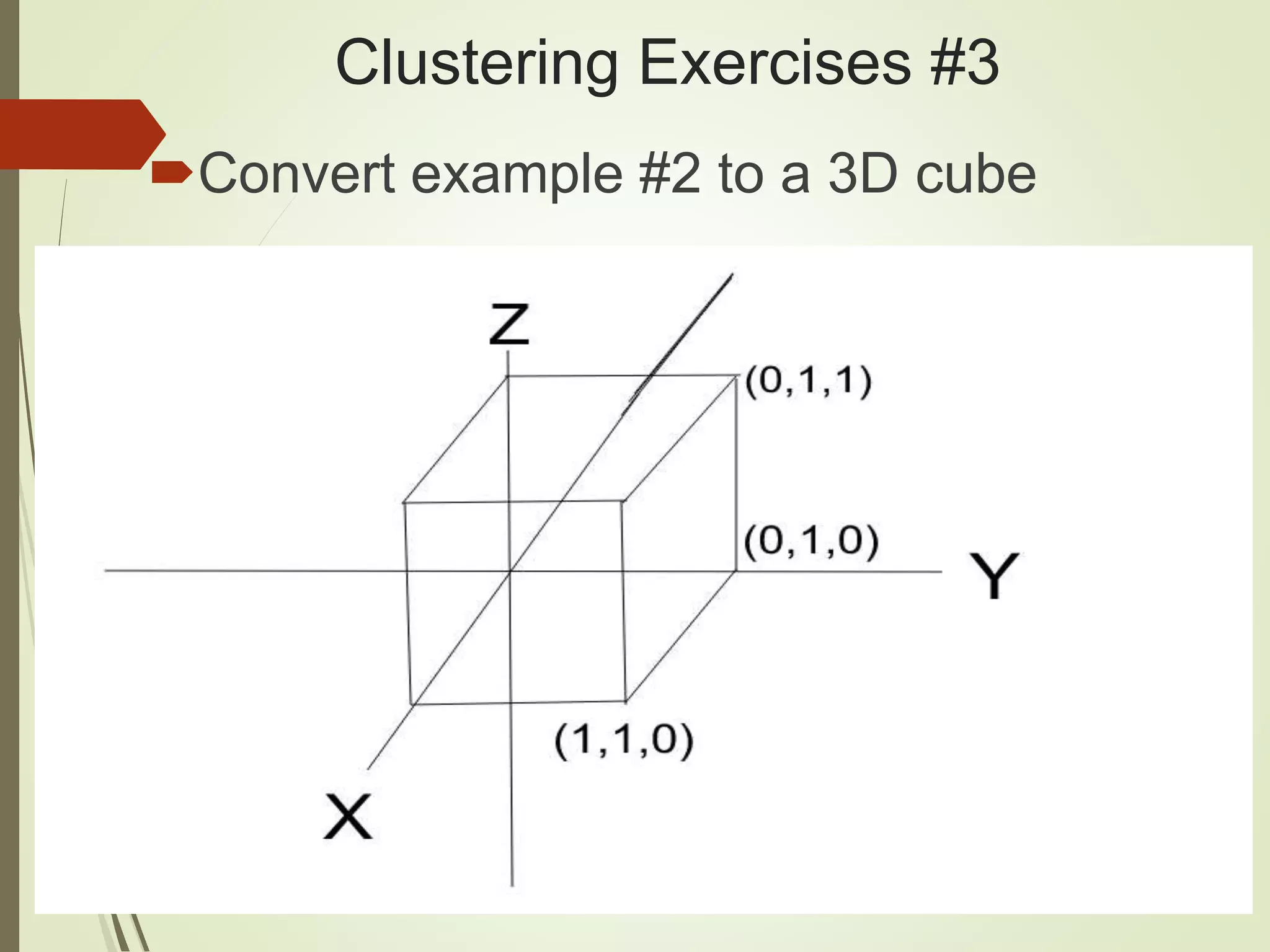
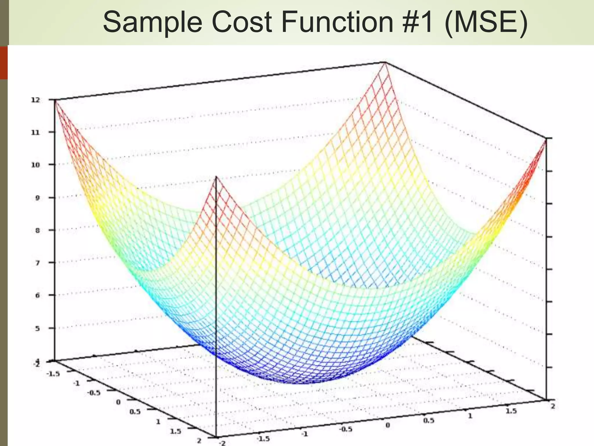
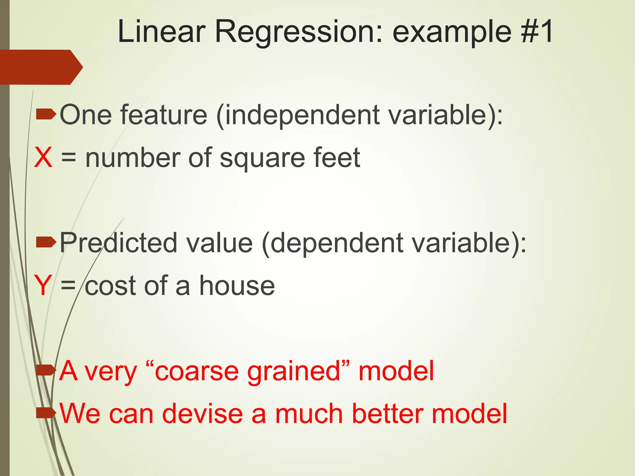
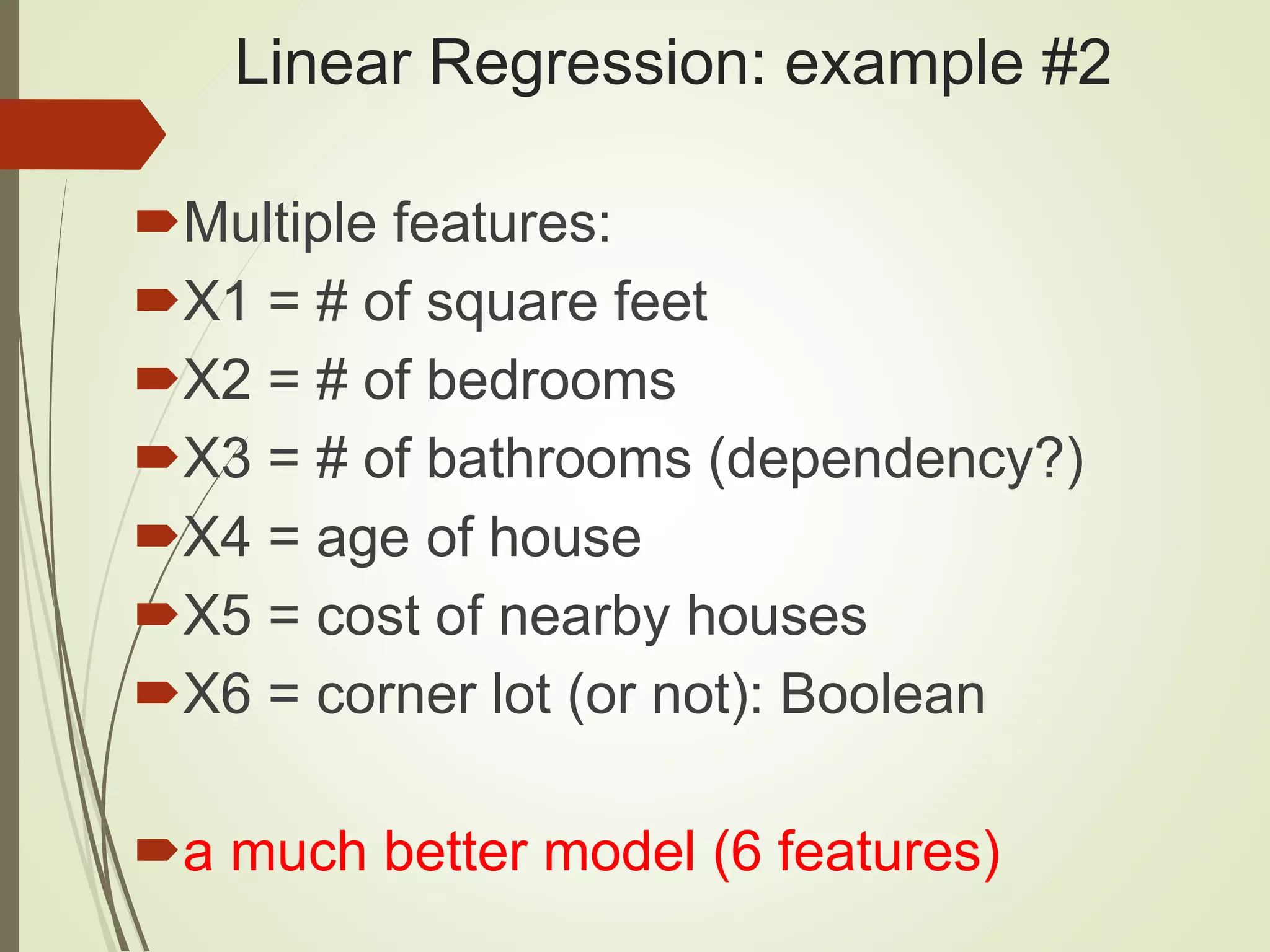
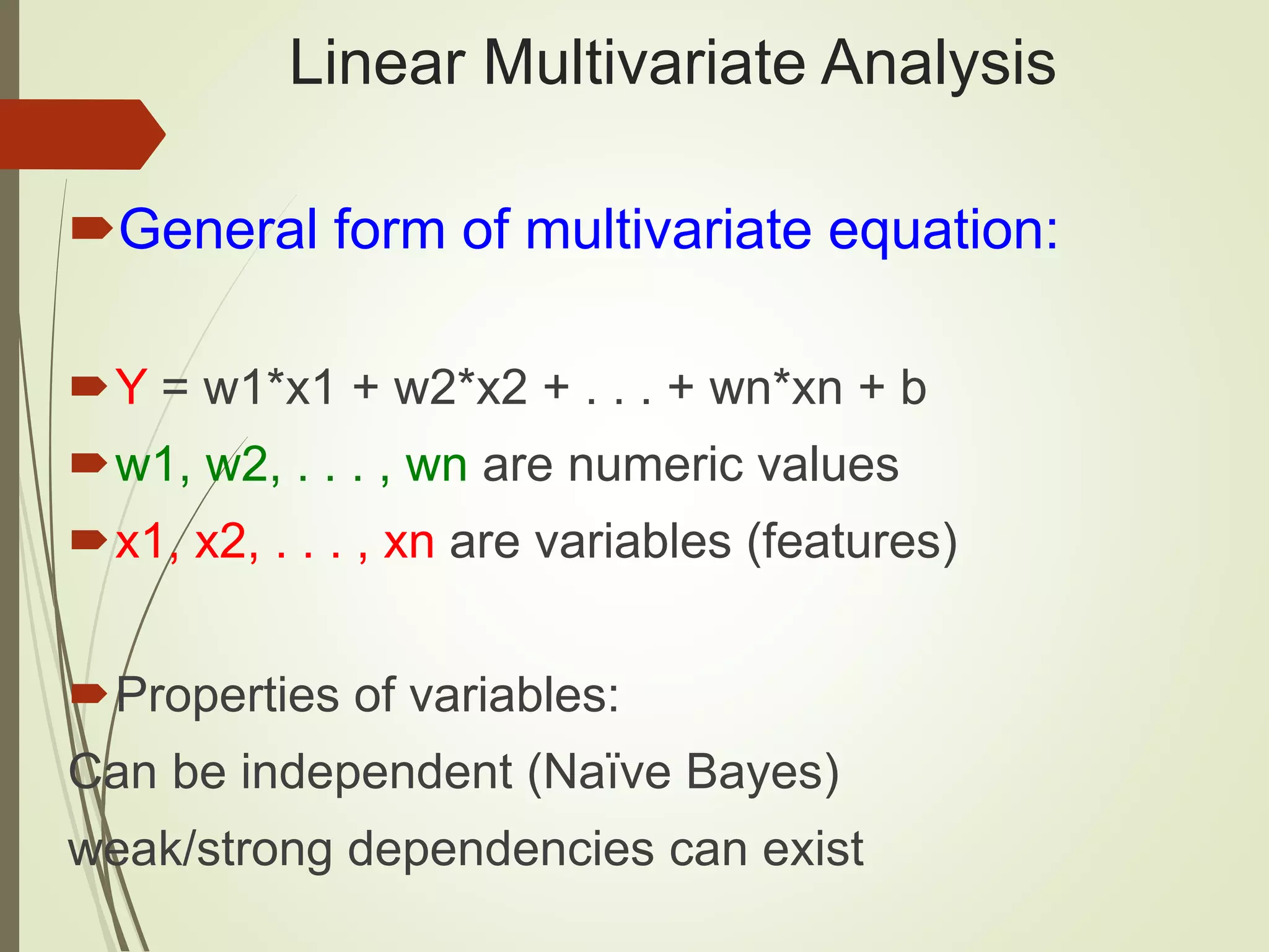
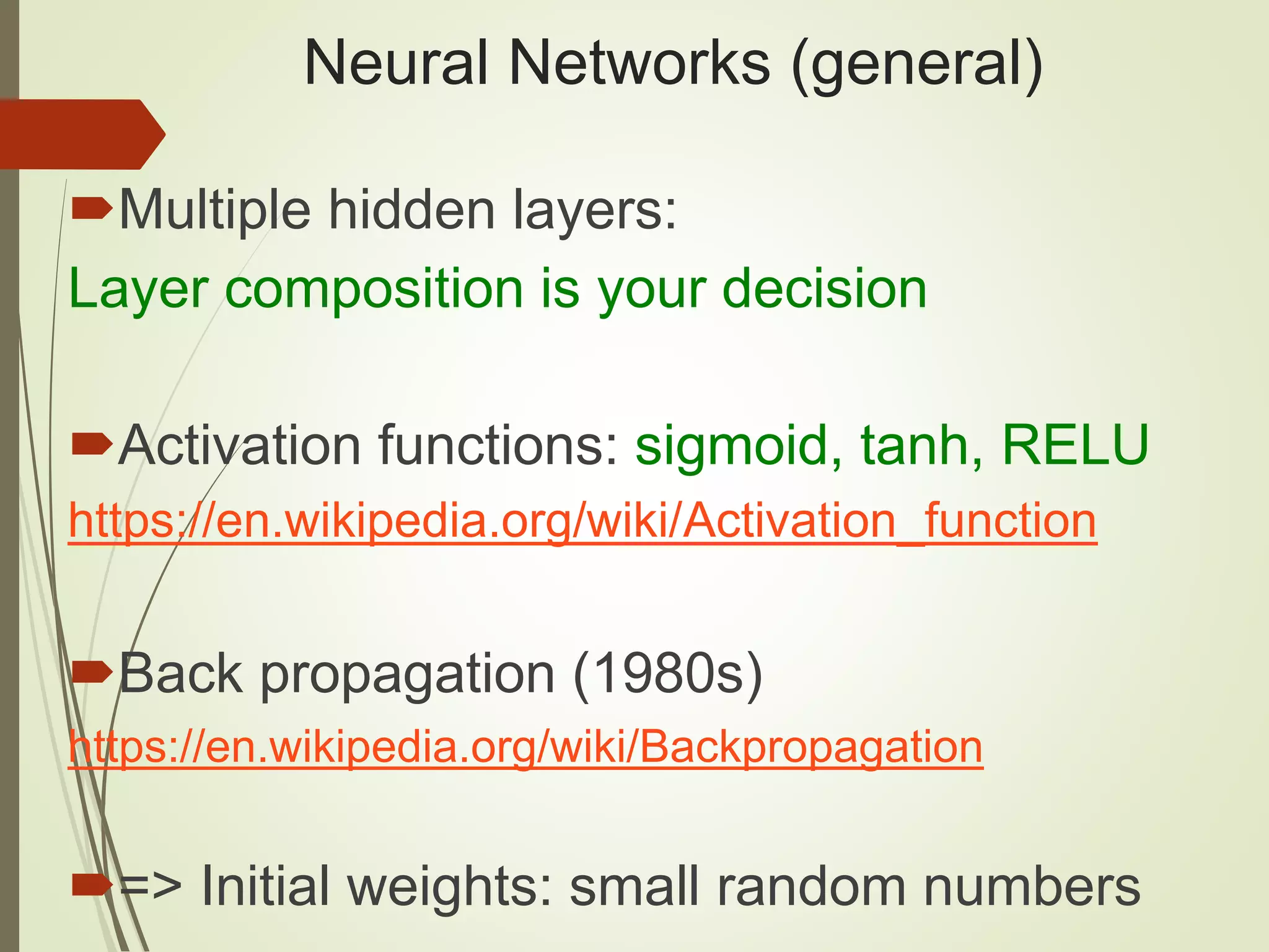
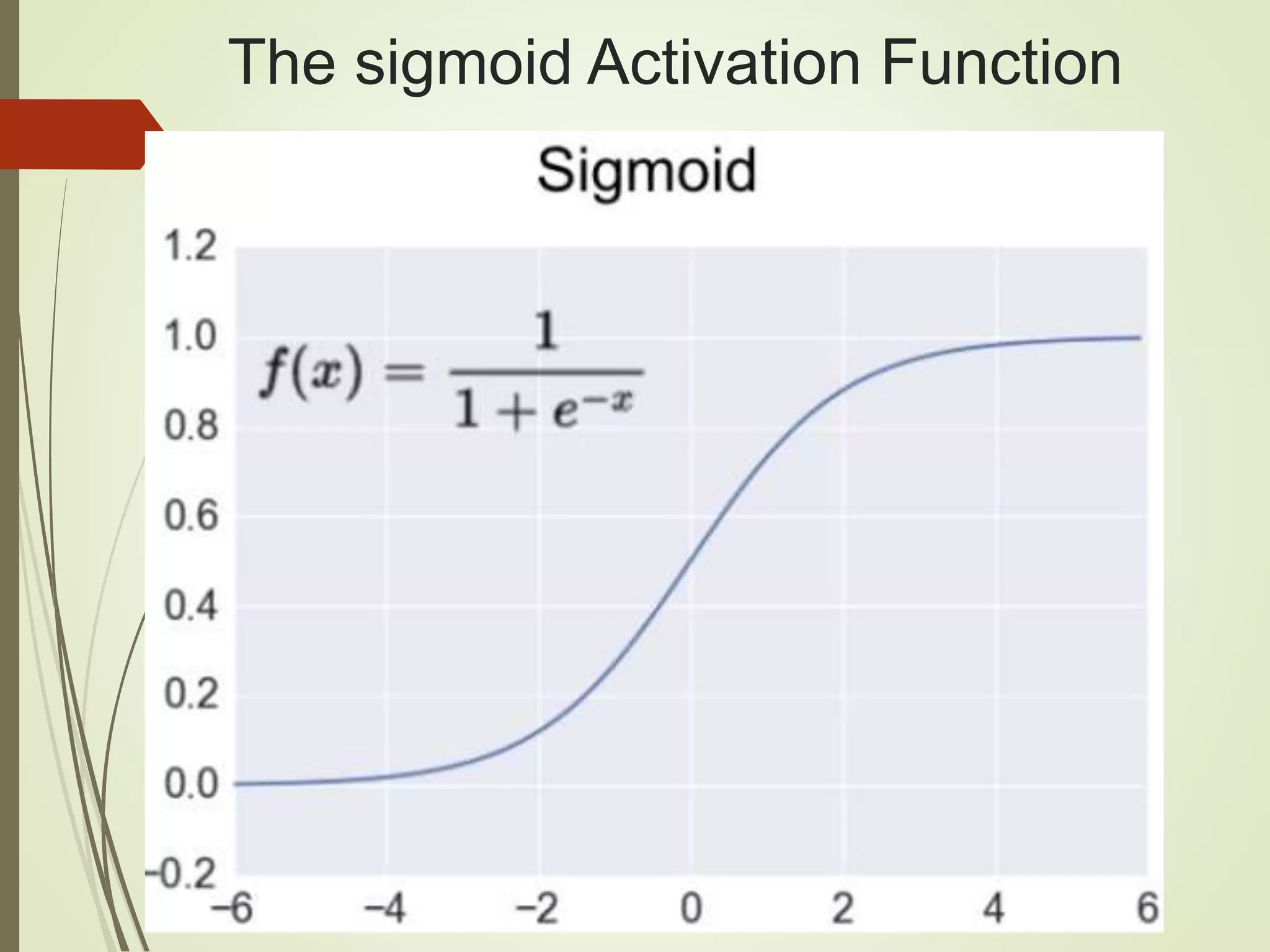
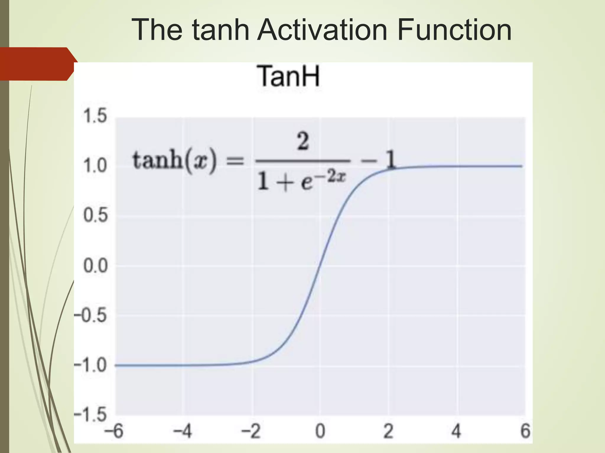
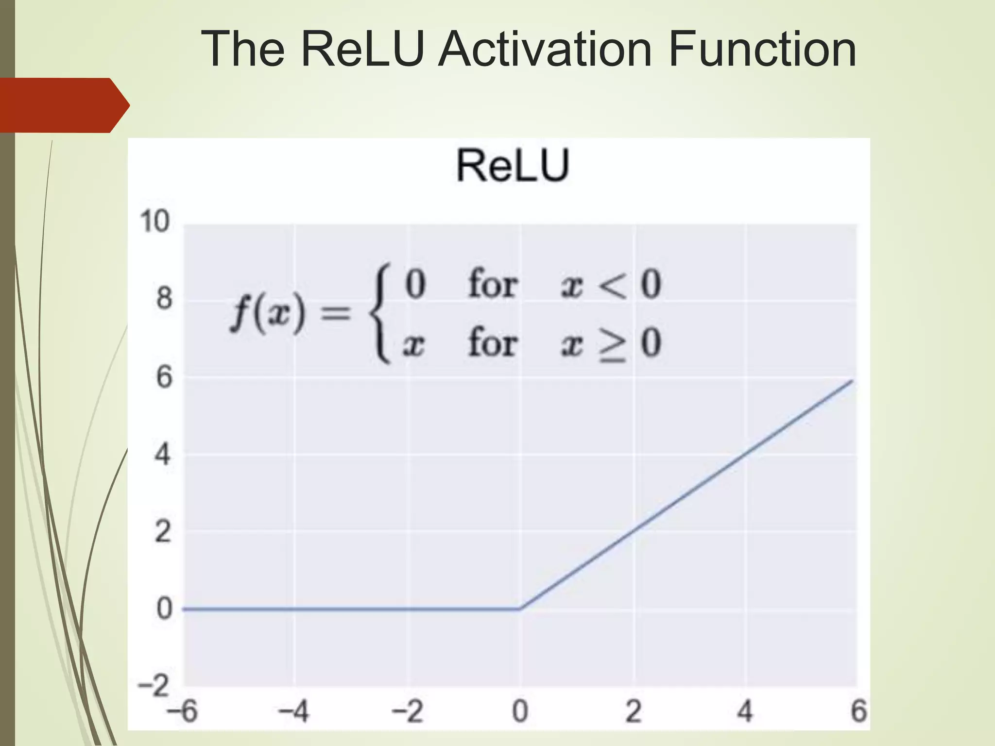
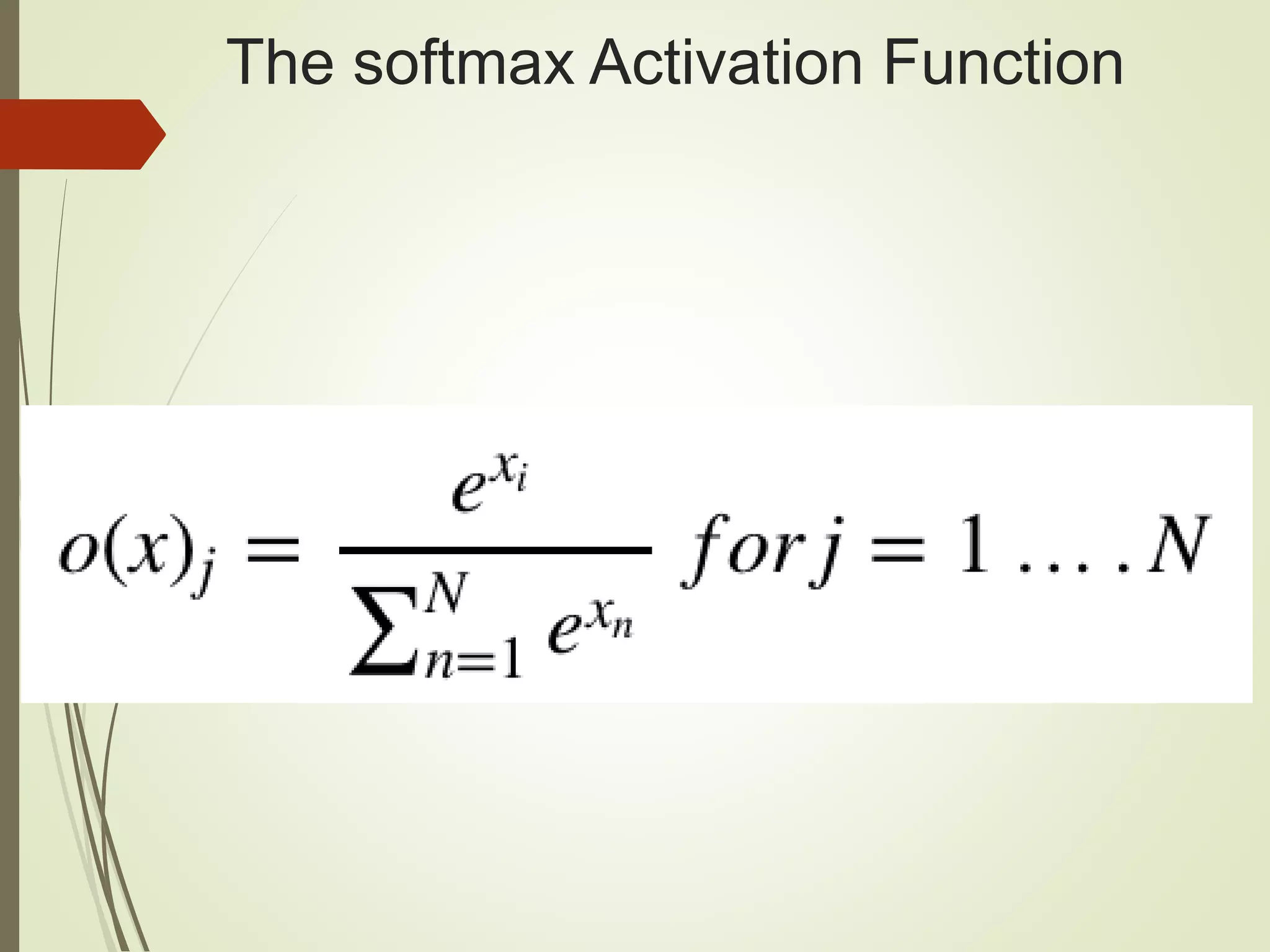
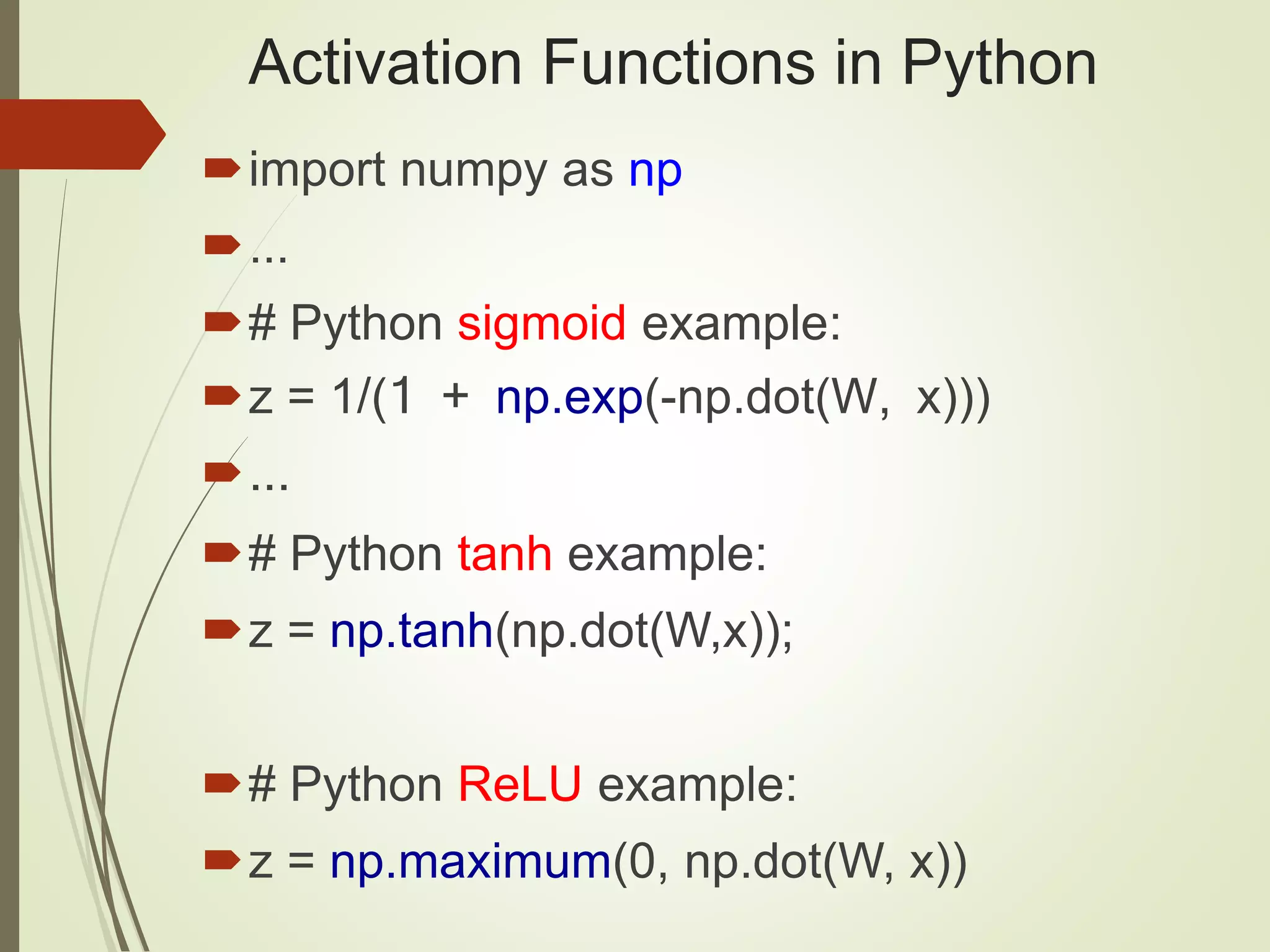
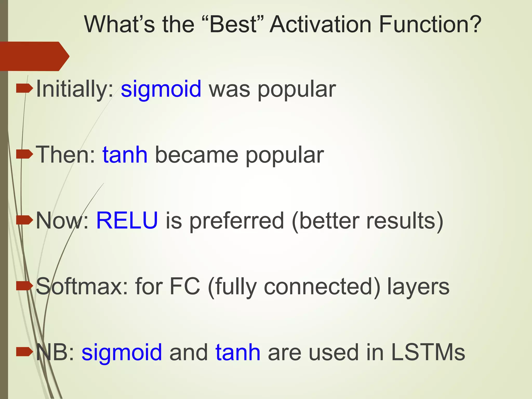
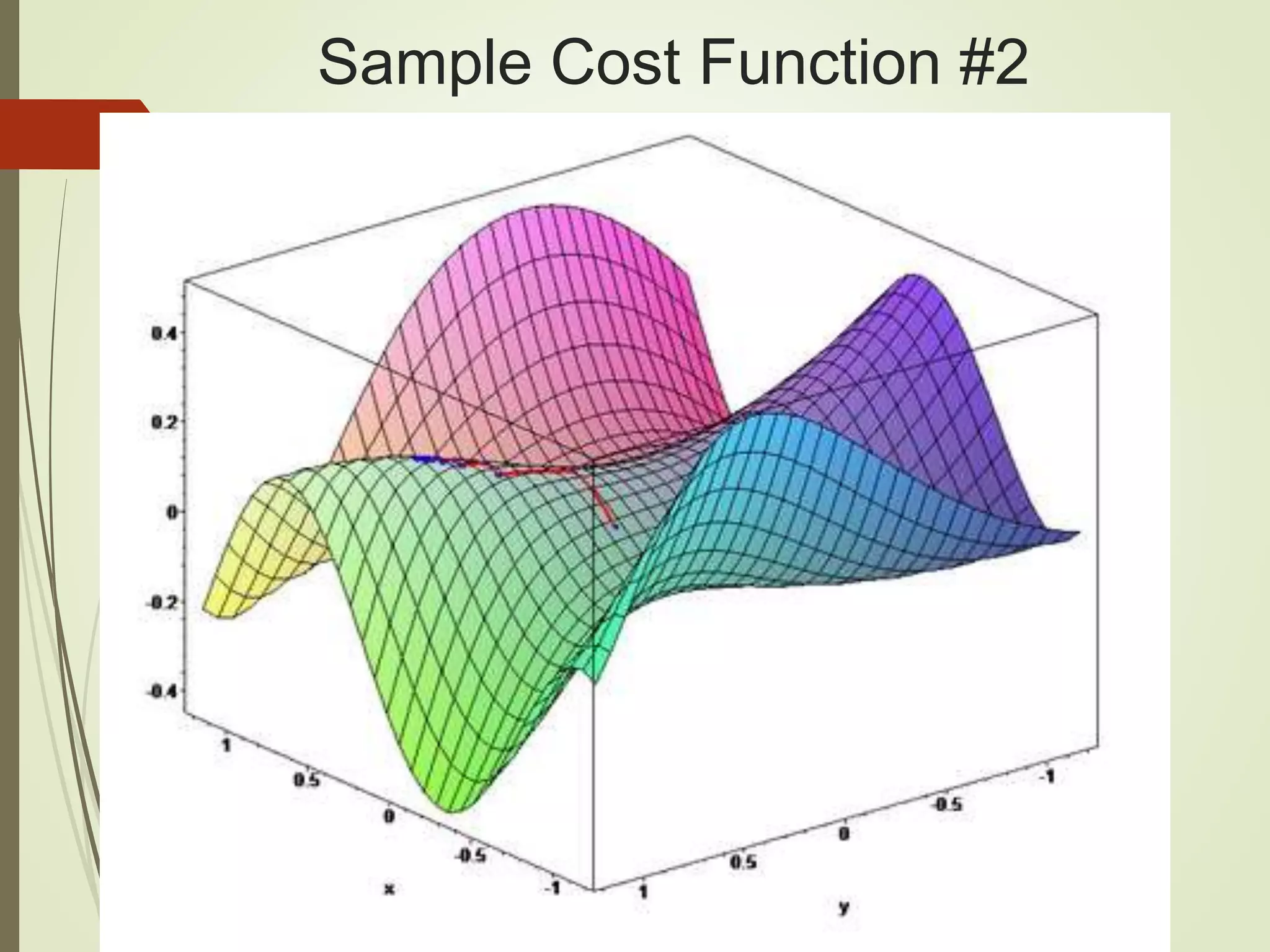
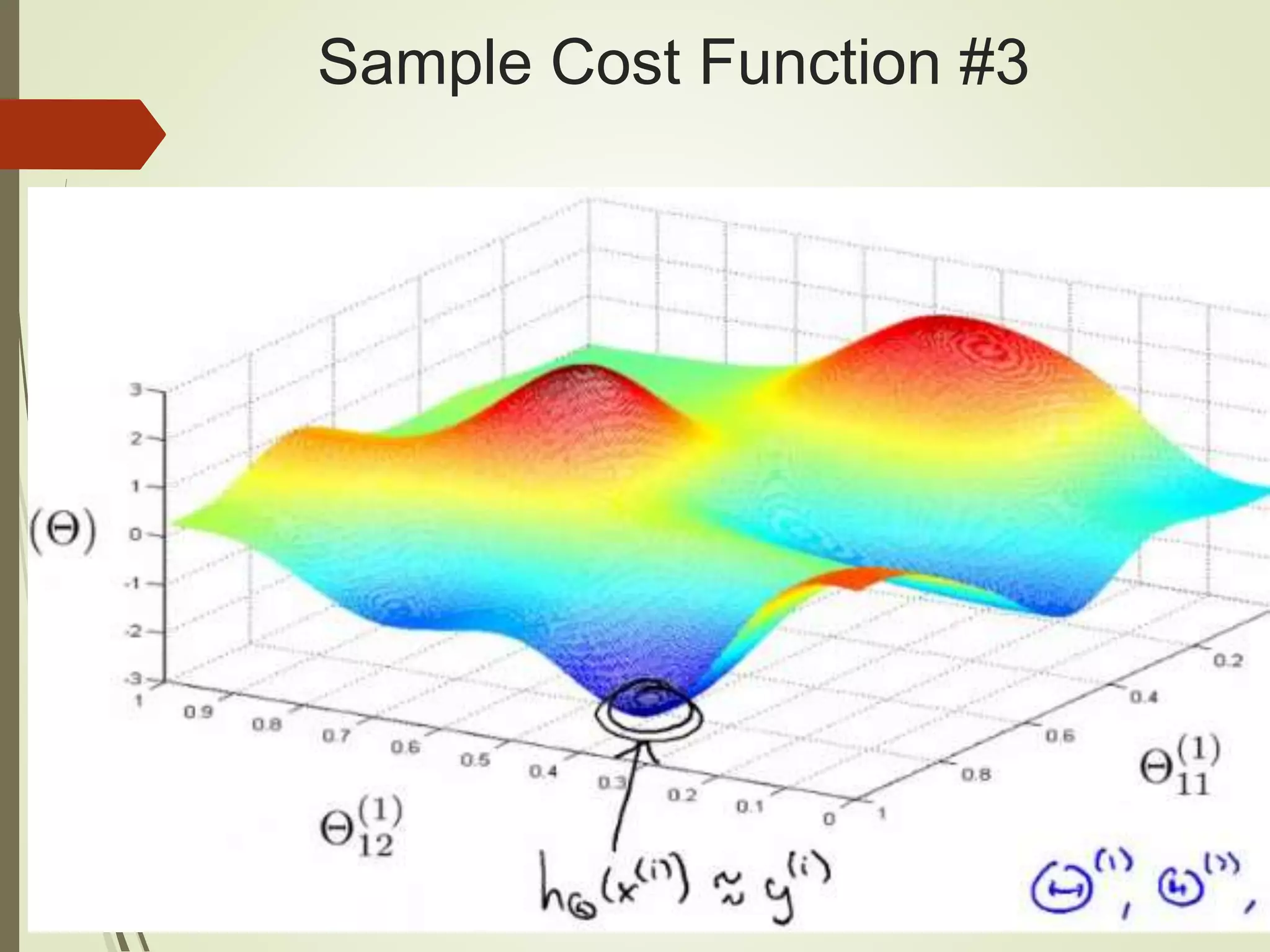
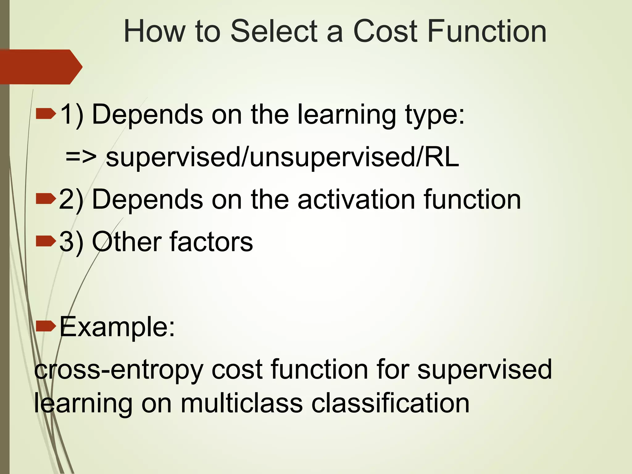
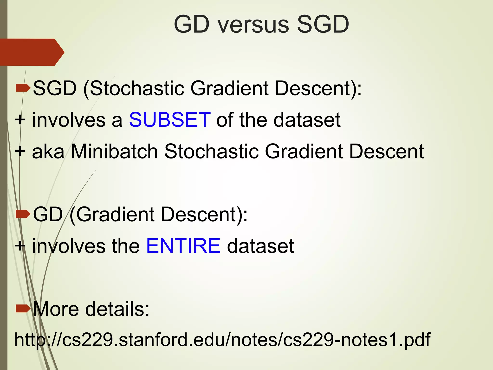
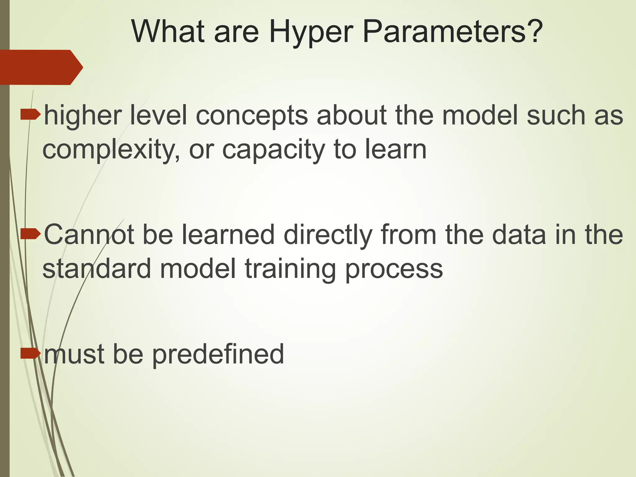
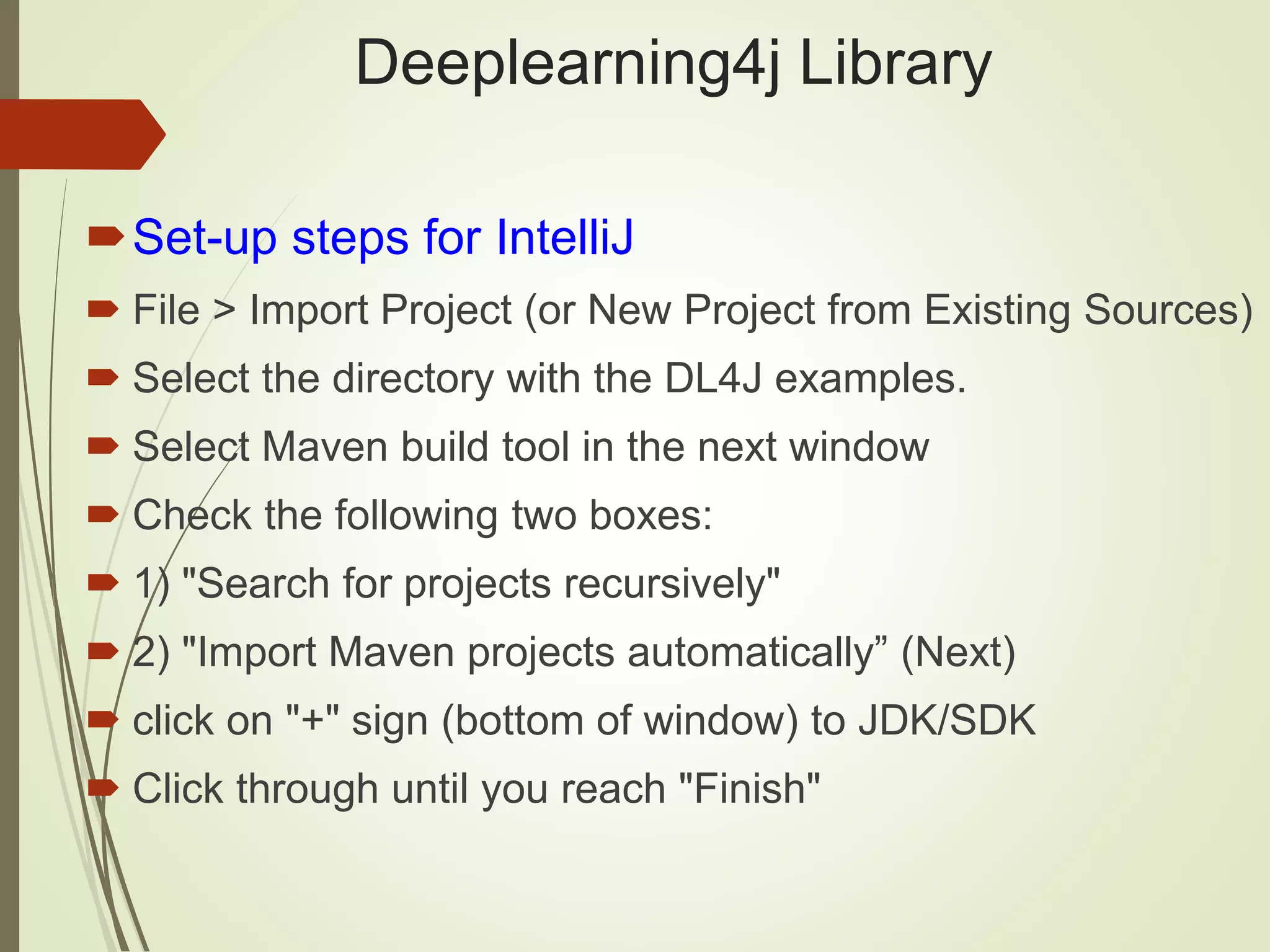
The document provides an overview of Java and deep learning concepts, including AI, machine learning, and neural networks. It covers various topics such as model representation, clustering examples, activation functions, gradient descent, deep learning frameworks like Deeplearning4j and TensorFlow, and practical coding examples. It also discusses the significance of hyperparameters and their role in optimizing machine learning models.