IRJET- A Study on Algorithms for FFT Computations

IRJET- A Study on Algorithms for FFT Computations

• 1.
  International Research Journalof Engineering and Technology (IRJET) e-ISSN: 2395-0056 Volume: 05 Issue: 10 | Oct 2018 www.irjet.net p-ISSN: 2395-0072 © 2018, IRJET | Impact Factor value: 7.211 | ISO 9001:2008 Certified Journal | Page 1487 A Study on Algorithms for FFT computations Saravanakumar Chandrasekaran1, Dr.G.Themozhi2 1Assistant Professor, Department of ECE, Valliammai Engineering College, Tamil Nadu 2Professor and Head, Department of ECE, Tagore Engineering College, Tamil Nadu ---------------------------------------------------------------------***---------------------------------------------------------------------- Abstract:- The Fast Fourier Transform is an qualified algorithm for computing the Discrete Fourier Transform in terms of reduced number of computations than that of direct evaluation of DFT. It has several applications in signal processing for frequency transformations. Because of the complexity of the FFT algorithm, recently various FFT algorithms have been proposed to meet real – time processing requirements and to reduce hardwarecomplexityoverthelast decades. So it is of considerable interest to researchers of signal processing technology to compare these algorithms. In this paper, a general analysis and comparison of the FFT algorithms is crisply done. The analysis of each algorithm includes the pace of the computation, amountofcomputations and memory requirements. Key Words: Fast Fourier Transform, Complexity, Comparison, Algorithm, Memory. 1. INTRODUCTION A sufficient number of FFT algorithms have been developed earlier for the efficient computation of the DFT. The first major breakthrough was the Cooley-Tukey algorithm [1] developed inthemid-sixtieswhichresultedina flood of works on FFTs. This algorithm reduced the complexity of a DFT fromO(N)toO(NlogN),whichatthetime wasaincredibleimprovementinefficiency.Algorithmswhich followed have achieved this complexity reduction to varying degrees. The Cooley-Tukey algorithm was a Radix-2 algorithm. The next few radixalgorithmsdevelopedwerethe Radix-3, Radix-4, and the Mixed Radix algorithm. Further research led to the Fast Hartley Transform (FHT) and the Split Radix (SPRAD) algorithm In this paper, from the literature we analyze each algorithm under a variety of constraints, and to use the statistics to create a best solution for the computation of FFT based on the constraints. 2. ALGORITHM 2.1 Radix 2 FFT Algorithm (RAD2) In computation of the N = 2n point DFT by the divide-and conquer approach., split the N-point data sequence into two N/2-point data sequences a1(n) and a2(n), corresponding to the even-numbered and odd-numbered samples of x(n), respectively, that is, a1(n) = x(2n) a2(n) = x(2n +1) , n = 0, 1,…..(N/2 – 1) Thus a1(n) and a2(n) are obtained by decimating x(n) by a factor of 2, and hence the resulting FFT algorithm is called a decimation-in-time algorithm. Now the N-point DFT can be expressed in terms of the DFT's of the decimated sequences as follows: But WN 2 = WN/2. With this substitution, the equation can be expressed as where F1(k) and F2(k) are the N/2-point DFTs of the sequences f1(m) and f2(m), respectively. Since F1(k) and F2(k) are periodic, with period N/2, we have F1(k+N/2) = F1(k) and F2(k+N/2) = F2(k). In addition, the factor WN k+N/2 = -WN k. Hence the equation may be expressed as It is observed that the direct computation of F1(k) requires (N/2)2 complex multiplications. It is also common to the computation of F2(k). Furthermore, thereare N/2additional complex multiplications required to compute WN kF2(k). Hence the computation of X(k) requires 2(N/2)2 + N/2 = N 2/2 + N/2 complex multiplications. This initial step fallout in a reduction of the number of multiplications from N2 to N 2/2 + N/2, which is about a factor of 2 for N large.
• 2.
  International Research Journalof Engineering and Technology (IRJET) e-ISSN: 2395-0056 Volume: 05 Issue: 10 | Oct 2018 www.irjet.net p-ISSN: 2395-0072 © 2018, IRJET | Impact Factor value: 7.211 | ISO 9001:2008 Certified Journal | Page 1488 2.2 Radix 4 FFT Algorithm (RAD4) When the number of data points N in the DFT is a power of 4 (i.e., N = 4v), always use a radix-2 algorithm for the computation. However, for this case, it is more proficient computationally to employ a radix-r FFT algorithm. In this algorithm, the N-point input sequenceisdecimatedintofour subsequences, x(4n), x(4n+1), x(4n+2), x(4n+3), n = 0, 1, ... , N/4-1. Thus the four N/4-point DFTs F(l, q)obtainedfromtheabove equation are collected together to arrive the N-point DFT. The expression for combining the N/4-point DFTs defines a radix-4 decimation-in-timebutterfly,whichcanbe expressed in matrix form as 2.3 Split Radix FFT Algorithm (SPRAD) The split-radix FFT, along with its variations, long had the distinction of achieving the lowest published arithmetic operation count (total exact number of required real additions and multiplications) to compute a DFT of power- of-two sizes N. The split-radix algorithm can only be applied when N is a multiple of 4, but since it breaks a DFT into smaller DFTs it can be combined with any other FFT algorithm as desired. 3. COMPARISON OF ALGORITHMS Typically, the primary touchstone criteria have been the number of mathematical operations (multiplications and additions), and/or the overall computation speed. The effectiveness of an algorithm is most affected by the arithmetic complexity, usually expressed in terms of a count of real multiplications and additions. However, on general purpose computers this is not a very good level and other factors need to be considered as well. For instance, the issue of memory usage is very important for memory constrained applications. 3.1 Amount of Computations As many CPUs have notably different speeds on floating point and integer operations, it is considered to individually account for floating point and integer arithmetic. It is a well known fact that most new architectures compute floating point operations more proficient than integer operations. Also, most indexing and loop control is done using integer arithmetic. Many FFT algorithms require a large number of division by-two operations which is competently accomplished by usingabinaryshiftoperator.Theresultsare referred from the literature. Table -1: Amount of Computation Algorithm Float Add Float Mul Int Add Int Mul Shift RAD2 14336 20480 19450 2084 1023 RAD4 8960 14336 12902 3071 277 SPRAD 5861 5522 12664 2542 1988 3.2 Pace of computation In most of the applications, for general purpose computers, with easy availability offasterCPUsandmemory not being a fore most constraint, the fastest algorithm is by far treated as the best algorithm. Thus, a common choice to rank algorithms is by their computation speed. Table -2: Pace of Computation Algorithm Order of FFT 16 64 256 1024 RAD2 20 60 260 1960 RAD4 20 60 300 1800 SPRAD 20 40 140 660 3.3 Memory Requirement In portable signal processing applications, the FFT is a core computational component. However, few applications cannot manage ahugememoryspaceforarrivingFFTs.While memory usage is important for specification of hardware, memory accesses also account for a significant portion of computation time. These observations from the literature insisted us to include memory usage as one of the criteria in deciding the effectiveness of the various FFT algorithms.
• 3.
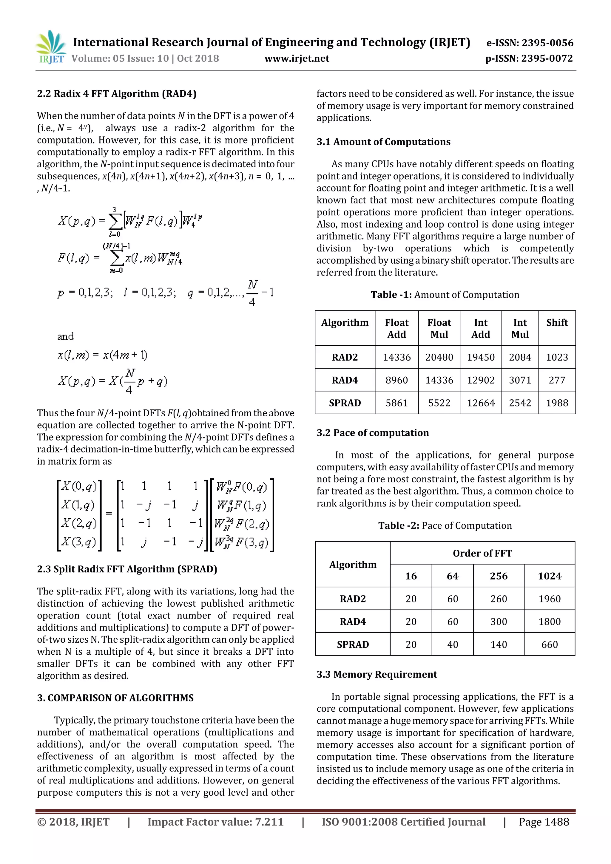
  International Research Journalof Engineering and Technology (IRJET) e-ISSN: 2395-0056 Volume: 05 Issue: 10 | Oct 2018 www.irjet.net p-ISSN: 2395-0072 © 2018, IRJET | Impact Factor value: 7.211 | ISO 9001:2008 Certified Journal | Page 1489 Table -3: Memory Requirements Algorithm Memory Requirement (Bytes) RAD2 72240 RAD4 72536 SPRAD 72508 4. CONCLUSIONS The amount of computation is graphically given below. The different arithmetic are compared. Chart -1: Amount of Computation For Shift operations, RAD 4 algorithm is best option if the constraint is number of computations. The pace of the computationreveals that SPRADalgorithmis best among the three. Chart -2: Pace of Computation The memory requirements are distributed equally for all the three algorithms. Chart -3: Memory Requirements REFERENCES [1] Manish Sone, Padma Kunthe, “A General comparison of FFT algorithms”, Cypress Semiconductors [2] J.W. Cooley and J.W. Tukey, (1965), An Algorithm for Machine Computation of Complex Fourier Series, Mathematical Computation, vol. 19, pp. 297-301. 2. R.N. Bracewell, (1985), TheHartleyTransform,OxfordPress, Oxford, England. [3] R.N. Bracewell, (1984), Fast Hartley Transform, Proceedings of IEEE, pp. 1010-1018. [4] H.S. Hou, (1987), The Fast HartleyTransformAlgorithm, IEEE Transactions on Computers, pp. 147-155, February. [5] P. Duhamel and H. Hollomann, (1984), Split Radix FFT Algorithm, Electronic Letters, vol. 20, pp.14-16,January [6] C.S. Burrus and T.W. Parks, (1985), DFT/FFT and Convolution Algorithms: Theory and Implementation, John Wiley and Sons, New York, NY, USA.