introduction to digital signal processing

Introduction to Digital Signal Processing UNIT 1

Dec 20, 2024 2 Contents Introduction to DSP Discrete time signals and sequences Linear Shift Invariant systems Stability and Causality Linear constant coefficient Difference equations Frequency domain representation of discrete time signals and systems

Dec 20, 2024 4 What is a Signal ? Anything which carries information is a signal. Examples  Human voice, chirping of birds, smoke signals, gestures (sign language), fragrances of the flowers.  Many of our body functions are regulated by chemical signals, blind people use sense of touch, ECG, EEG  Bees communicate by their dancing pattern.

Dec 20, 2024 5 Some examples of modern high speed signals  Voltage charger in a telephone wire  Electromagnetic field emanating from a transmitting antenna,  Variation of light intensity in an optical fiber. In this course we will learn some of the mathematical representations of the signals A signal is a real (or complex) valued function of one or more real variable(s)

Dec 20, 2024 6 A continuous-time signal x (t) (discrete-time signal x[n]) is a function of an independent continuous variable t (discrete variable n)

Dec 20, 2024 7 Classification of signals a) Based on no of independent variables  1D : When the function depends on a single variable, the signal is said to be one dimensional. EX : A speech signal, daily maximum temperature, annual rainfall at a place  MULTIDIMENSIONAL : When the function depends on two or more variables, the signal is said to be multidimensional.

Dec 20, 2024 8 Images (2D): light intensity as a function of 2D coordinates Black and white or grey scale images (I=0-255) Colour images: I=red(0-255), green(0-255), blue(0-255) Video (3D) : Sequence of images, called frames Is a function of 3 variables = 2 spatial coordinates and time Our physical world is four dimensional ( Three spatial and one temporal) EX: speed of wind , pressure etc.,

Dec 20, 2024 9 Classification of signals b) Based on nature of independent variables  Continuous signals  Discrete signals Time Amplitude analog signals continuous-time signals discrete-time signals digital signals Continuous Continuous Discrete Discrete A signal is said to be continuous when it is defined for all instants of time

Dec 20, 2024 11 Digital signals that are discrete in time and quantized in amplitude Discrete time signals are defined for discrete instances of time Amplitude is continuous

Dec 20, 2024 13 Classification of signals contd.. c) Based on nature of indeterminacy  Deterministic signals  Random signals d) Based on periodicity e) Based on causality f) Based on energy content in signal g) Natural or synthetic signals

Dec 20, 2024 14 Need for processing To obtain signal in more desirable form (transformation of signal) or interpretation and manipulation of signals Ex: Noise cancellation, Multiplexing and demultiplexing Amplification of signals

Dec 20, 2024 16 Signal Process Systems analog system signal output continuous-time signal continuous-time signal discrete- time system signal output discrete-time signal discrete-time signal digital system signal output digital signal digital signal ASP DSP

Dec 20, 2024 17 ASP : In Classical radio, Telephone, Radar and Television systems For signals that are not digitized

Dec 20, 2024 19  Digital Signal Processors (DSP) take real-world (natural) signals like voice, audio, video, temperature, pressure, or position that have been digitized and then mathematically manipulate them.  A DSP is designed for performing mathematical functions like "add", "subtract", "multiply" and "divide" very quickly. What is a Digital Signal Processing ?

Dec 20, 2024 21 Advantages of Digital Signal Processing (1) Flexibility : Same hardware can be used to do various kind of signal processing operation. while in the analog signal processing one has to design a system for each kind of operation. (2) Repeatability : The same signal processing operation can be repeated again and again giving same results while in analog systems there may be parameter variation due to change in temperature or supply voltage.

Dec 20, 2024 22 (3) High Accuracy : The accuracy of the analog filter is affected by the tolerance of the circuit components used for design the filter, but DSP has superior control of accuracy. (4) Flexibility in Configuration : For reconfiguring an analog system, we can only do it by redesign of system hardware, where as a DSP System can be easily reconfigured only by changing the program. (5) Ease of Data Storage : On magnetic media, without the loss of fidelity the digital signals can be stored and can be processed off-line in a remote laboratory.

Dec 20, 2024 23 (6) Time Sharing : The cost of the processing signal can be reduced in DSP by the sharing of a given processor among a number of signals. (7) Cheaper : The digital realization is much cheaper than the analog realization in many applications. (8) Stability : Less sensitive environmental changes (9) Applicable for very low frequency signal processing e.g. seismic signals

Dec 20, 2024 24 Disadvantages of Digital Signal Processing (1) Power Consumption : The DSP chip consists of over 4 Lakh transistors, which will yields to dissipate high power (1 Watt), whereas the analog signal processing includes only passive circuit elements like resistors, capacitors and inductors, which will leads to only low power dissipation. (2) Processing of signals beyond higher frequencies (beyond GHz) and below lower frequencies (a few Hz) involves limitations

Dec 20, 2024 25 (3) Information is lost because we only take samples of the signal at intervals . (4) Speed is limited and increased complexity due to A/D and D/A Converters (5) Frequency range of operation is limited due to sampling Disadvantages of Digital Signal Processing

Discrete-Time Signals--- Sequences Discrete-Time Signals and Systems

Sampling Of Low Pass Signal Let m(t) be a base band signal which is band limited and its highest frequency component is fM. Let the values of m(t) be determined at regular intervals separated by Ts ≤ 1/2 fM,that is the signal is periodically sampled for every Ts seconds .Then these samples m(nTS),where n is an integer,uniquely determine the signal and the signal may be reconstructed from these samples with no distortion. The time Ts is called Sampling Time Dec 20, 2024 28

Dec 20, 2024 33 Representation of sequences

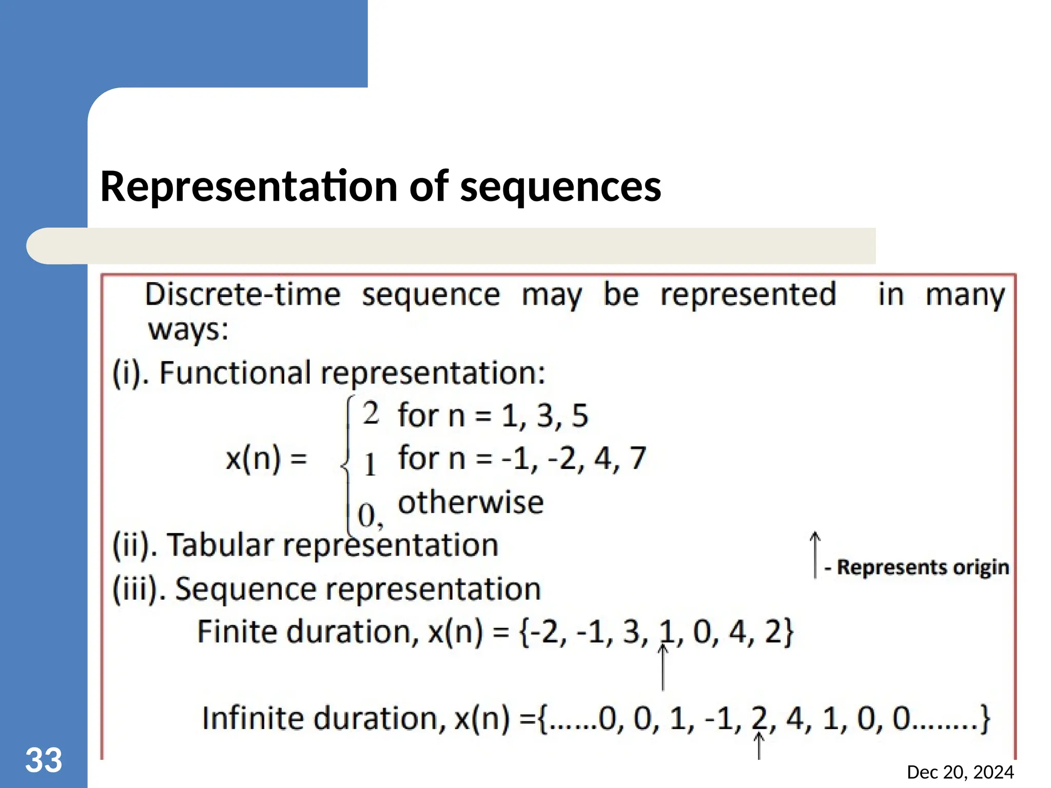
 Tabular Representation Ggraph Dec 20, 2024 34 1 2 3 4 5 6 7 8 9 10 -1 -2 -3 -4 -5 -6 -7 -8 n x[n]

Dec 20, 2024 35 Elementary discrete-time signals / sequences 1. Unit sample sequence or Unit impulse or Kronecker delta function (much simpler than the Dirac impulse)

Dec 20, 2024 36 2. unit step sequence

Dec 20, 2024 38 3. Unit Ramp sequence 4. Signum Function

Dec 20, 2024 39 5. Exponential Function

Dec 20, 2024 40 6. Sinusoidal sequence

Dec 20, 2024 41 Periodic only if

Dec 20, 2024 42 Classification of discrete-time signals 1.Periodic and Aperiodic sequence N, m must be integers P1: Determine whether or not each of the following signals is periodic. If a signal is periodic, specify its fundamental period Always periodic Not periodic always

Dec 20, 2024 43 2.Symmetric (Even) and Anti Symmetric (odd) sequence For an Even signal x(n) = x(-n) For an odd signal x(-n) = -x(n) P2.Find the odd and even components of x(n) For even part

Dec 20, 2024 45 3. Power or Energy sequence The energy of a discrete-time signal is defined as The average power of a signal is defined as If E is finite, [0 ≤ E < ] and P = 0 then x(n) is called an energy signal ꝏ The average power of periodic sequence with period N is given by If E is infinite and If P is finite and nonzero, then x[n] is called a power signal.

Dec 20, 2024 46 P4. Determine the power & energy of the unit step sequence. P5. Test whether the given signal is an energy signal or a power signal. x[n] = 5 (a constant signal)

Dec 20, 2024 47 Operations on Sequences 1. Amplitude Scaling: (A Constant Multiplier) 2.Addition of two signals (An Adder)

Dec 20, 2024 48 3. The product of two signals (A signal Multiplier) 4. Shifting A unit delay element A unit advance element Time shifting y[n] = x[n − k]. k can be positive (delayed signal) or negative (advanced signal)

Dec 20, 2024 50 5. Folding or reflection or time-reversal y[n] = x[−n]

Dec 20, 2024 51 x(n − 2) x(−n) x(2 − n) Try x(-2 - n) Try x(-2 + n)

Dec 20, 2024 52 6. Time-scaling Down sampling /compression Up sampling /expansion

Dec 20, 2024 53 x(n) = u(n + 3) + 0.5 u(n − 1) x(n) = δ(n + 3) + 0.5 δ(n − 1) x(n) = 2^n · δ(n − 4) x(n) = 2^n · u(−n − 2) x(n) = (−1)^n . u(−n − 4) x(n) = 2 δ(n + 4) − δ(n − 2) + u(n − 3) Practice problems Make an accurate sketch of each of the discrete-time signals

Dec 20, 2024 54 Make an accurate sketch of each of the discrete-time signals

Linear Shift Invariant systems Discrete-Time Signals and Systems

Dec 20, 2024 56  A device or an algorithm that performs some prescribed operation on a discrete time signal (input or excitation) to produce another discrete time signal (output or response) Discrete-time system y[n] = T {x[n]} Accumulator system     n k k x n y ) ( ) ( Ideal Delay System ) ( ) ( d n n x n y   Squarer  2 ] [ ) ( n x n y  Compressor ] [ ) ( Mn x n y  Examples T [ ] x[n] y[n] = T [ x[n] ]

Dec 20, 2024 57  Adder  Constant multiplier  Signal multiplier  Unit delay element (why z −1 clear later) How are delays implemented?. Block diagram representation of discrete-time systems With buffers / latches / flip-flops

Dec 20, 2024 58 Classification of discrete-time systems  Linear & non-linear systems  Time-variant & Time-Invariant systems  Static & Dynamic systems  Causal & noncausal systems  Stable & unstable systems Time properties (causality, memory, time invariance) Amplitude properties (stability, invertibility, linearity)

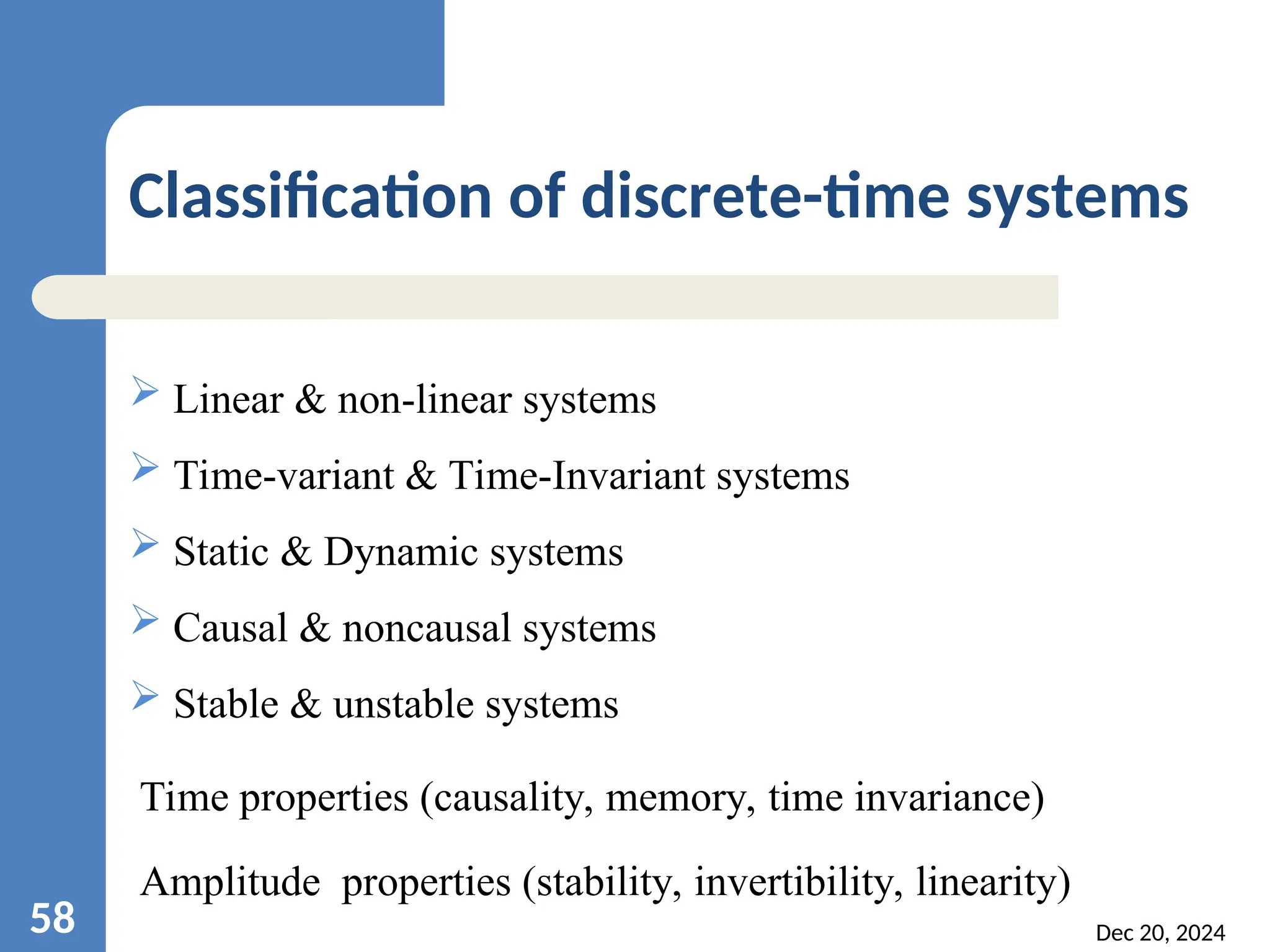
Dec 20, 2024 59 1. Linear & non-linear systems System is said to be linear if it obeys superposition principle 1. Homogeneity or scaling property 2. Additivity property These two properties together comprise the principle of superposition T {a x[n] } = a T{ x[n] } If a = 0 we see that zero input signal implies zero output signal for a linear system T { x1 [n] + x2 [n] } = T { x1 [n] } + T { x2 [n] }

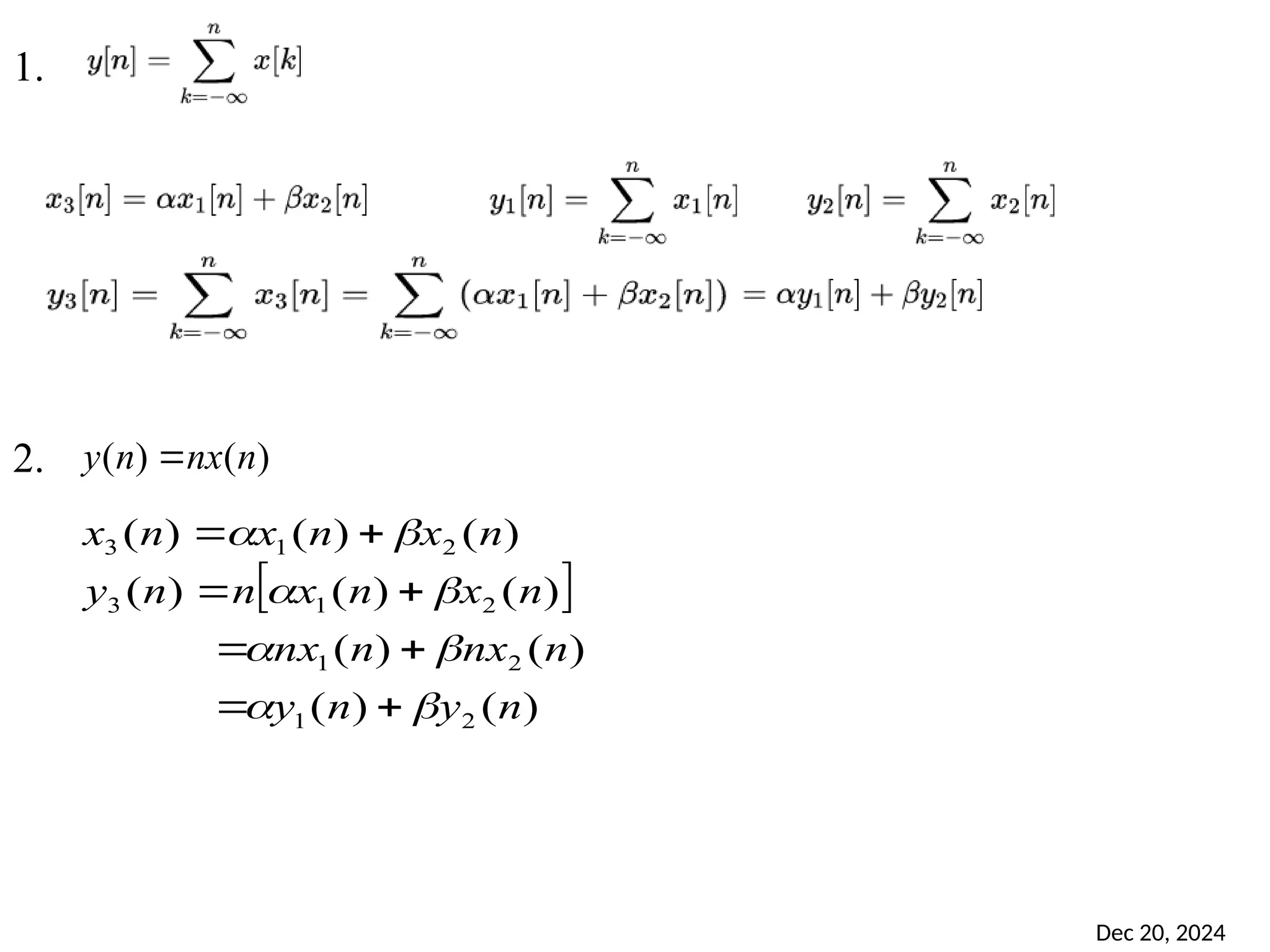
Dec 20, 2024 60 A system T is linear iff T { α x1[n] + β x2[n] } = α T { x1[n] } + β T { x2[n] } x3[n] = α x1[n] + β x2[n] = T { x3[n] } α α β β T T T

Dec 20, 2024 61 Determine whether the system given below are linear or non-linear. ) ( ) ( n x n y  ) ( ) ( 2 n x n y  ) ( ) ( n nx n y    ) ( cos ) ( n x n y  ) ( ) ( n x n y    ) ( log ) ( n x n y 

Dec 20, 2024 62 1. 2. ) ( ) ( n nx n y    ) ( ) ( ) ( ) ( ) ( ) ( ) ( ) ( ) ( ) ( 2 1 2 1 2 1 3 2 1 3 n y n y n nx n nx n x n x n n y n x n x n x                

Dec 20, 2024 63 2. Time-variant & Time-Invariant systems Systems whose input-output behavior does not change with time are called Time-invariant A relaxed system T is called Time Invariant or Shift Invariant iff implies that Graphically:

Dec 20, 2024 64 ) ( ) ( ) ( ) , ( k n x n x at n y k n y    k n n n y k n y     ) ( ) ( 1. y(n) = x(-n) 2. y(n) = x(n) + x(n-1) 3. y(n) = n x(n) 4. y(n) = x(2n) 5. y(n) = x(n) sinω0n If delayed output is equal to output due to delayed input then system is said to be Shift-invariant

Dec 20, 2024 65 1. y(n) = x(2n) 2. y(n) = x(n) sinω0n

Dec 20, 2024 67 3. Static & Dynamic systems  For a Static system or Memory less system, the output y[n] depends only on the current input x[n], not on previous (n-1) or future (n+1) inputs .  Output depends on past, present & future samples of I/P - Dynamic (with memory) Ex

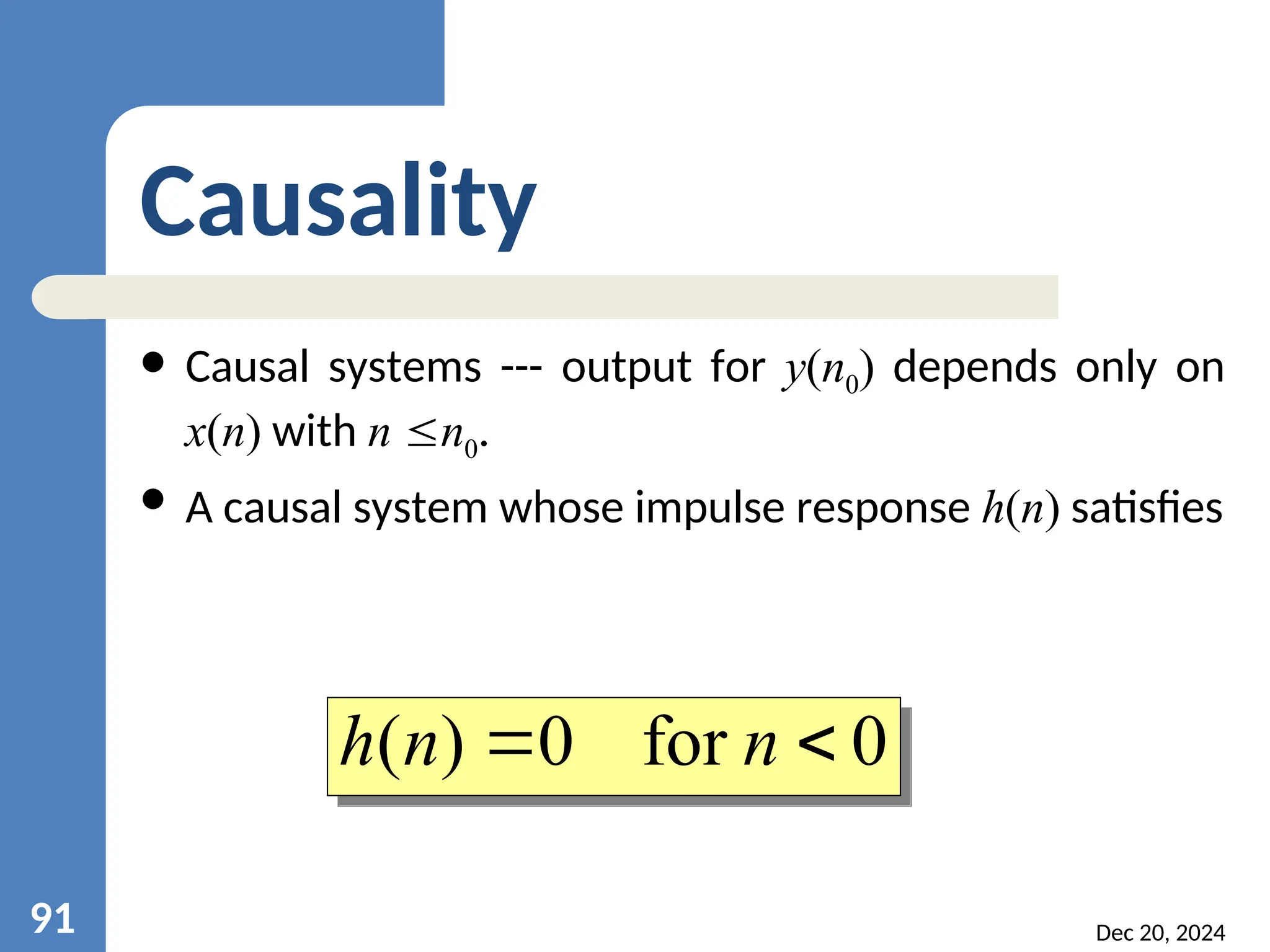
Dec 20, 2024 68 4. Causal & NonCausal systems  For a Causal system, the output y[n] at any time n depends only on the “ present ” and “ past ” inputs i.e., y(n) = x(n)+u(n+1)  Non causal system – The system does not satisfy the above condition. y(n) = x(-n) y(n) = x(2n) For n < n0 ; i.e., n=1, n0=4 y(n) = ax(n)+b Ex Ex

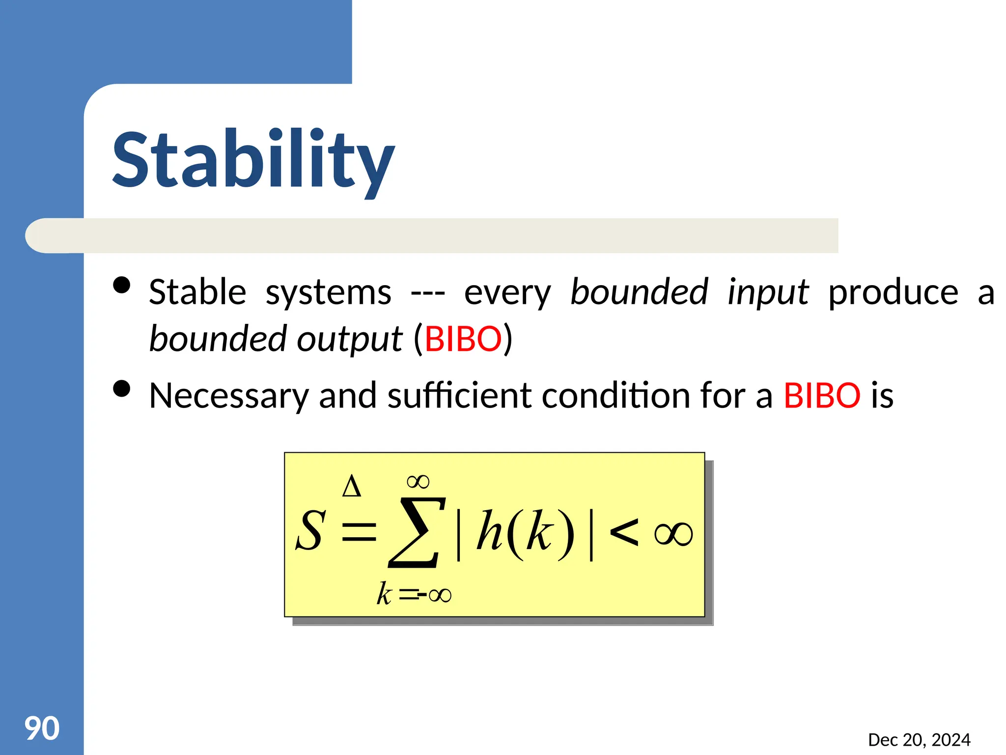
Dec 20, 2024 69 5. Stable & unstable systems  A system is Bounded-Input Bounded-Output (BIBO) stable iff every bounded input produces a bounded output If ∃ Mx s.t. | x[n] | ≤ Mx < ∞ n, then there must exist an ∀ My s.t. | y[n] | ≤ My < ∞ n ∀ unstable k n x n y stable k n x m n y unstable n n x n y k n k            0 1 0 2 ) ( ) ( ) ( 1 ) ( ) ( ) ( Ex

Dec 20, 2024 70 Analysis of Linear Time Invariant systems Why analysis? So far we only have input-output relationships. For a given system can compute y[n] for selected x[n]’s , but very difficult to design filters etc LTI h (n)

Dec 20, 2024 71  Decompose input signal x[n] into a weighted sum of elementary Two particularly good choices for the elementary functions • impulse functions δ [n − k] • complex exponentials  Determine response of system to each elementary  Apply superposition property: Techniques for the analysis of linear systems

Dec 20, 2024 72 Resolution of discrete-time signal into impulses This is the sifting property of the unit impulse function x(n) = {0.5, 1.5, 0, -1, 1, 0.75, 2} x(n) = 0.5 δ(n+2)+1.5 δ(n+1)-δ(n-1)+δ(n-2)+0.75 δ(n-3)+2 δ(n-4) T [ ] (n) h(n) x(n) y(n) Impulse Response

Dec 20, 2024 73 Let the symbol h[n-k] to denote the system output when the input is δ[n − k] , i.e., Because the system is Time Invariant system Response of LTI systems to arbitrary inputs: The Convolution Sum T [ ] x(n) y(n) = T [x(n)] ) ( ) ( ) ( k n k x n x k                    ) ( ) ( ) ( k n k x T n y k  ) ( )] ( [ k n h k n T    

Dec 20, 2024 74 )] ( [ ) ( ) ( k n T k x n y k        ) ( ) ( k n h k x k       Delayed Impulse as input Delayed Impulse Response             ) ( ) ( ) ( k n k x T n y k  ) ( * ) ( n h n x  convolution The convolution sum shows that with the impulse response h[n], you can compute the output y[n] for any input signal x[n] . Thus A LTI system is characterized completely by its impulse response h[n]

Dec 20, 2024 75 Properties of Convolution ) ( * ) ( ) ( ) ( ) ( n h n x k n h k x n y k        ) ( * ) ( ) ( ) ( ) ( n x n h k n x k h n y k        Convolution is Commutative ) ( * ) ( ) ( * ) ( n x n h n h n x  If x[n] has n = N1, . . . , N1 + L1 − 1 (length L1) and h[n] has n = N2, . . . , N2 + L2 − 1 (length L2) then y[n] = x[n] h[n] has L = L1 + L2 − 1 ∗

Dec 20, 2024 76 Convolution is Associative h1(n) x(n) h2(n) y(n) h2(n) x(n) h1(n) y(n) h1(n)*h2(n) x(n) y(n) These three systems are identical. Convolution is Associate

1. Given x[n] and h[n], choose an initial value of n, the starting time for evaluating the output sequence y[n]. If x[n] starts at n = n1 and h[n] starts at n = n2 then n = n1+n2 is a good choice. 2. Express both the sequences in terms of the index k to get h[k] and x[k]. 3. Tilt h[k] about k=0 to obtain h[-k] and shift by n to the right if n is positive and left if n is negative to obtain h[n- k]. Dec 20, 2024 77 Convolution Process steps ) ( ) ( ) ( k n h k x n y k      

4. Multiply the two sequences x[k] and h[n-k] element by element and sum the products to get y[n]. 5. Increment the index n, shift the sequence h[n-k] from left to right by one sample and repeat step-4. 6. Repeat step-5 until the sum of products is zero for all remaining values of n. Dec 20, 2024 78 Convolution Process steps ) ( ) ( ) ( k n h k x n y k      

Dec 20, 2024 79 Example.1 ]. [ * ] [ ] [ } 2 , 1 , 2 , 1 { ] [ } 2 , 1 , 2 , 3 { ) ( n h n x n y find n h and n x Given     ] [n h y(n)=? 0 1 2 3 4 5 6 n 0 1 2 3 4 5 6 n -1 3 2 1 2 1 1 2 2

Dec 20, 2024 80 Example.1 n1= 0, n2= -1  n = n1+n2= -1 0 1 2 3 4 5 6 k x[k] -1 0 1 2 3 4 5 k h[k] 1 2 3 4 5 6 7 k h[-k] 0 -2 -1 } 2 , 1 , 2 , 1 { ] [ } 2 , 1 , 2 , 3 { ) (    n h and n x 3 1 . 3 ) 1 ( ) ( ) 1 (           k h k x y k 1 2 3 4 5 6 7 k h[-1-k] 0 -2 -1 -3 ) ( ) ( ) ( k n h k x n y k       3 2 1 2 1 1 2 2 1 1 2 2 2 1 1 2

Dec 20, 2024 81 Example.1 0 1 2 3 4 5 6 k x[k] -1 0 1 2 3 4 5 k h[k] 1 2 3 4 5 6 7 k h[-k] 0 -2 -1 8 2 6 1 . 2 2 . 3 ) ( ) ( ) 0 (            k h k x y k ) ( ) ( ) ( k n h k x n y k       3 2 1 2 1 1 2 2 n = -1+1=0 2 1 1 2 } 2 , 1 , 2 , 1 { ] [ } 2 , 1 , 2 , 3 { ) (    n h and n x

Dec 20, 2024 82 Example.1 0 1 2 3 4 5 6 k x[k] -1 0 1 2 3 4 5 k h[k] 1 2 3 4 5 6 7 k h[1-k] 0 -2 -1 8 1 . 1 2 . 2 1 . 3 ) 1 ( ) ( ) 1 (           k h k x y k ) ( ) ( ) ( k n h k x n y k       n = 0+1=1 1 2 3 4 5 6 7 k h[-k] 0 -2 -1 2 1 1 2 3 2 1 2 1 1 2 2 2 1 1 2 } 2 , 1 , 2 , 1 { ] [ } 2 , 1 , 2 , 3 { ) (    n h and n x

Dec 20, 2024 83 Example.1 0 1 2 3 4 5 6 k x[k] -1 0 1 2 3 4 5 k h[k] 1 2 3 4 5 6 7 k h[2-k] 0 -2 -1 12 1 . 2 2 . 1 1 . 2 2 . 3 ) 2 ( ) ( ) 2 (            k h k x y k 3 2 1 2 1 1 2 2 1 2 3 4 5 6 7 k h[-k] 0 -2 -1 2 1 1 2 2 1 1 2 ) ( ) ( ) ( k n h k x n y k       n = 1+1=2 } 2 , 1 , 2 , 1 { ] [ } 2 , 1 , 2 , 3 { ) (    n h and n x

Dec 20, 2024 84 Example.1 0 1 2 3 4 5 6 k x[k] -1 0 1 2 3 4 5 k h[k] h[3-k] 1 2 3 4 5 6 7 k 0 -2 -1 9 2 . 2 1 . 1 2 . 2 ) 3 ( ) ( ) 3 (           k h k x y k 3 2 1 2 1 1 2 2 1 2 3 4 5 6 7 k h[-k] 0 -2 -1 2 1 1 2 2 1 1 2 ) ( ) ( ) ( k n h k x n y k       n = 2+1=3 } 2 , 1 , 2 , 1 { ] [ } 2 , 1 , 2 , 3 { ) (    n h and n x

Dec 20, 2024 85 Example.1 0 1 2 3 4 5 6 k x[k] -1 0 1 2 3 4 5 k h[k] h[4-k] 1 2 3 4 5 6 7 k 0 -2 -1 4 1 . 2 2 . 1 ) 4 ( ) ( ) 4 (          k h k x y k 3 2 1 2 1 1 2 2 1 2 3 4 5 6 7 k h[-k] 0 -2 -1 2 1 1 2 2 1 1 2 ) ( ) ( ) ( k n h k x n y k       n = 3+1=4 } 2 , 1 , 2 , 1 { ] [ } 2 , 1 , 2 , 3 { ) (    n h and n x

Dec 20, 2024 86 Example.1 0 1 2 3 4 5 6 k x[k] -1 0 1 2 3 4 5 k h[k] h[5-k] 1 2 3 4 5 6 7 k 0 -2 -1 4 2 . 2 ) 5 ( ) ( ) 5 (         k h k x y k 3 2 1 2 1 1 2 2 1 2 3 4 5 6 7 k h[-k] 0 -2 -1 2 1 1 2 2 1 1 2 ) ( ) ( ) ( k n h k x n y k       n = 4+1=5 n1= 3, n2= 2  n = n1+n2= 5 } 2 , 1 , 2 , 1 { ] [ } 2 , 1 , 2 , 3 { ) (    n h and n x

Dec 20, 2024 87 Example.1 0 1 2 3 4 5 6 n y[n ] -1 ) ( ) ( ) ( k n h k x n y k       } 2 , 1 , 2 , 1 { ] [ } 2 , 1 , 2 , 3 { ) (    n h and n x 3 8 8 12 9 4 4 } 4 , 4 , 9 , 12 , 8 , 8 , 3 { ) (   n y

Stability and Causality Linear Time Invariant systems

Dec 20, 2024 90 Stability  Stable systems --- every bounded input produce a bounded output (BIBO)  Necessary and sufficient condition for a BIBO is        k k h S | ) ( |

Dec 20, 2024 91 Causality  Causal systems --- output for y(n0) depends only on x(n) with n n0.  A causal system whose impulse response h(n) satisfies 0 for 0 ) (   n n h

Dec 20, 2024 92 Example:  Show that the linear shift-invariant system with impulse response h(n)=an u(n) where |a|<1 is stable.              1 1 | ) ( | 0 k k k a a k h S

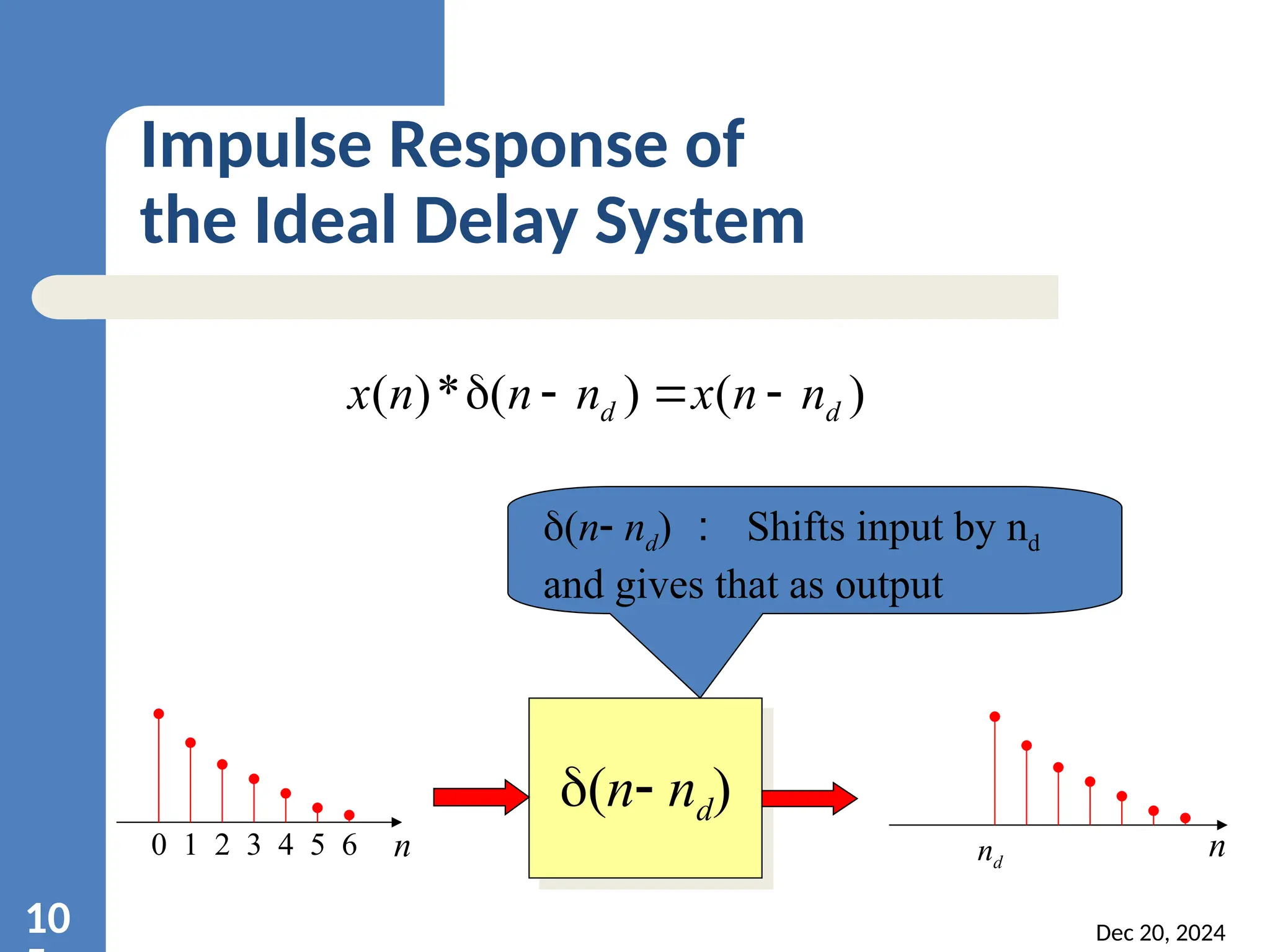
Dec 20, 2024 93 Example: Ideal Delay System ) ( ) ( d n n x n y   Accumulator     n k k x n y ) ( ) ( Moving Average        2 1 ) ( 1 1 ) ( 2 1 M M k k n x M M n y T [ ] x(n ) y(n)=T[x(n) ]  Check the following systems for stability and causality

Dec 20, 2024 94 Example: Squarer  2 ] [ ) ( n x n y  Forward difference ] [ ] 1 [ ) ( n x n x n y    Compressor eger ve is M n Mn x n y int , ], [ ) (        T [ ] x(n ) y(n)=T[x(n) ]  Check the following systems for stability and causality Backward difference ] 1 [ ] [ ) (    n x n x n y

Solution Select x1[n]=x2[n] for n≤k x1[n]≠x2[n] for n>k Find T{x1[n]}=x1[n-nd] and T{x2[n]}=x2[n-nd] At n=k T{x1[n]}= T{x2[n]} if nd is positive So system is causal for nd≥0 System is noncausal for nd<0 If x[n]<∞ .i.e. M, bounded input y[n] also bounded . So system is stable. Dec 20, 2024 95 Ideal Delay System ) ( ) ( d n n x n y  

Solution Select x1[n]=x2[n] for n≤k x1[n]≠x2[n] for n>k T{x1[n]}= and T{x2[n]}= T{x1[n]}= T{x2[n]} if M1≤0 and M2>-M1 Then the system is causal otherwise the system is noncausal Dec 20, 2024 96 Moving Average system        2 1 ) ( 1 1 ) ( 2 1 M M k k n x M M n y       2 1 ) ( 1 1 1 2 1 M M k k n x M M       2 1 ) ( 1 1 2 2 1 M M k k n x M M

Solutions If x[n]<∞ .i.e. M bounded input then output y[n] also bounded. So the system is stable. Dec 20, 2024 97 Moving Average        2 1 ) ( 1 1 ) ( 2 1 M M k k n x M M n y M M M M M M M M M n y then M n x If M M k              2 1 1 ) 1 ( 1 1 ] [ ] [ 2 1 2 1 2 1

Dec 20, 2024 98 Example.2 0 1 2 3 4 5 6 ) ( ) ( ) ( N n u n u n x          0 0 0 ) ( n n a n h n y(n)=? 0 1 2 3 4 5 6 n n

Dec 20, 2024 99 Example ) ( ) ( ) ( * ) ( ) ( k n h k x n h n x n y k        0 1 2 3 4 5 6 k x(k) 0 1 2 3 4 5 6 k h(k) 0 1 2 3 4 5 6 k h(0k)

Dec 20, 2024 10 Example ) ( ) ( ) ( * ) ( ) ( k n h k x n h n x n y k        0 1 2 3 4 5 6 k x(k) 0 1 2 3 4 5 6 k h(0k) 0 1 2 3 4 5 6 k h(1k) compute y(0) compute y(1) How to computer y(n)?

Dec 20, 2024 10 Example ) ( ) ( ) ( * ) ( ) ( k n h k x n h n x n y k        0 1 2 3 4 5 6 k x(k) 0 1 2 3 4 5 6 k h(0k) 0 1 2 3 4 5 6 k h(1k) compute y(0) compute y(1) How to computer y(n)? Two conditions have to be considered. n<N and nN.

Dec 20, 2024 10 Example ) ( ) ( ) ( * ) ( ) ( k n h k x n h n x n y k        1 1 1 ) 1 ( 0 0 1 1 1 ) (                    a a a a a a a a a n y n n n n k k n n k k n n < N n  N 1 1 1 0 1 0 1 1 1 ) (                     a a a a a a a a a n y N n n N n N k k n N k k n

Dec 20, 2024 10 Example ) ( ) ( ) ( * ) ( ) ( k n h k x n h n x n y k        1 1 1 ) 1 ( 0 0 1 1 1 ) (                    a a a a a a a a a n y n n n n k k n n k k n n < N n  N 1 1 1 0 1 0 1 1 1 ) (                     a a a a a a a a a n y N n n N n N k k n N k k n 0 2 4 6 0 5 10 15 20 25 30 35 40 45 50

Dec 20, 2024 10 Impulse Response of the Ideal Delay System Ideal Delay System ) ( ) ( d n n x n y   ) ( ) ( d n n n h    By letting x(n)=(n) and y(n)=h(n), (n nd) 0 1 2 3 4 5 6 nd n n

Dec 20, 2024 10 Impulse Response of the Ideal Delay System (n nd) 0 1 2 3 4 5 6 nd ) ( ) ( * ) ( d d n n x n n n x     (n nd) ： Shifts input by nd and gives that as output n n

Dec 20, 2024 10 Impulse Response of the Moving Average Moving Average        2 1 ) ( 1 1 ) ( 2 1 M M k k n x M M n y        2 1 ) ( 1 1 ) ( 2 1 M M k k n M M n h             otherwise M n M for M M n h 0 1 1 ) ( 2 1 2 1 M1  0  M2 . . . . . . Sequence of (n k) n

Dec 20, 2024 10 Impulse Response of the Accumulator ) ( ) ( ) ( n u k n h n k       Unit-step function Accumulator     n k k x n y ) ( ) ( 0 . . . n

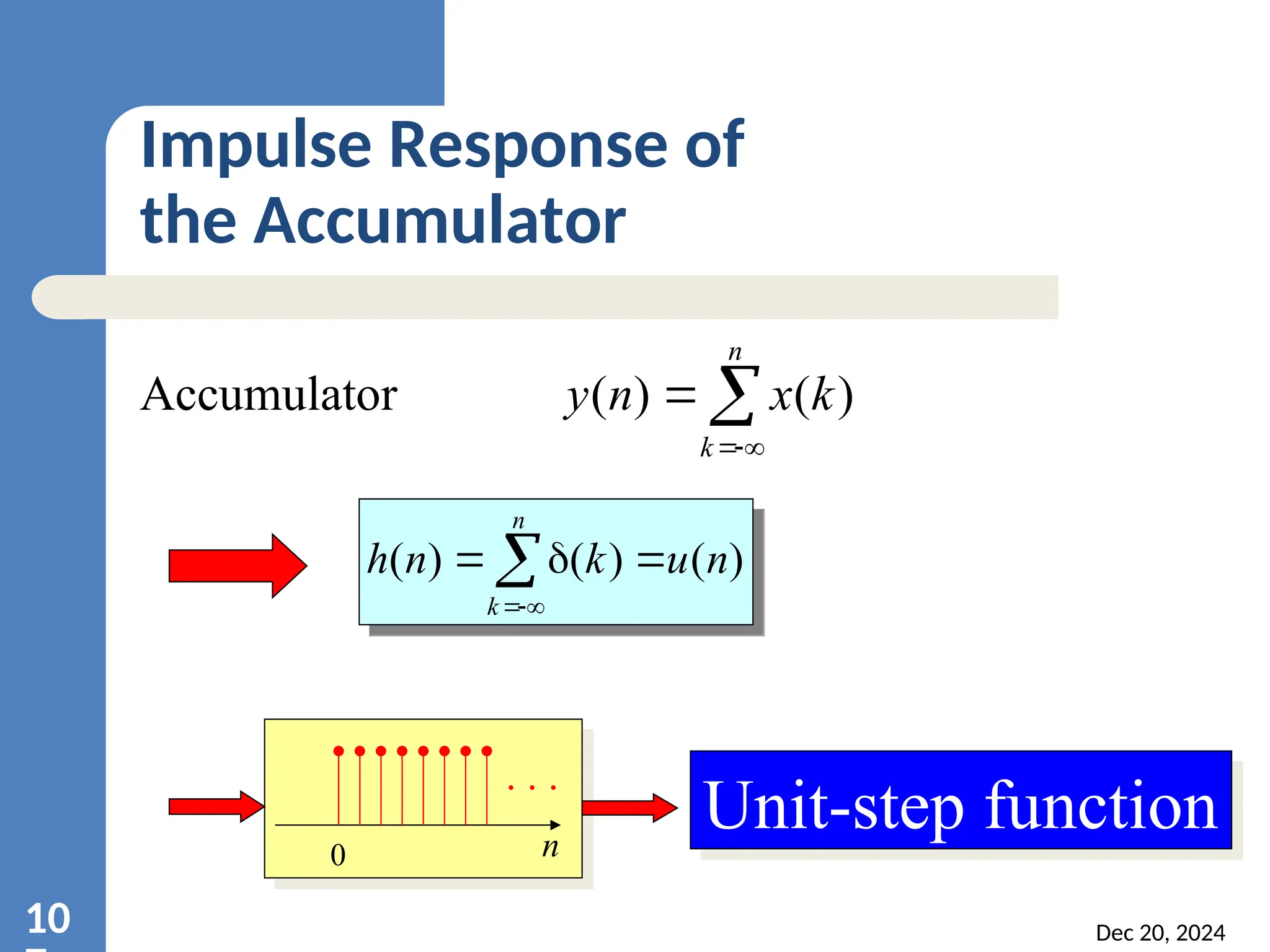
Solutions Select x1[n]=x2[n] for n≤k x1[n]≠x2[n] for n>k T{x1[n]}= and T{x2[n]}= T{x1[n]}= T{x2[n]} so the system is causal. So the system is unstable. Dec 20, 2024 10 Accumulator     n k k x n y ) ( ) (    n k k x ) ( 1    n k k x ) ( 2        n k M n y then M n x If ] [ ] [

Linear Constant-Coefficient Difference Equations Discrete-Time Signals and Systems

Dec 20, 2024 11 Nth Order Difference Equations        M k k N k k k n x b k n y a 0 0 ) ( ) ( Examples: Ideal Delay System ) ( ) ( d n n x n y   Accumulator ) ( ) 1 ( ) ( n x n y n y    Moving Average      M k k n x M n y 0 ) ( 1 1 ) (

Dec 20, 2024 11 Compute y(n)        M k k N k k k n x b k n y a 0 0 ) ( ) (          M k k N k k k n x a b k n y a a n y 0 0 1 0 ) ( ) ( ) (

Dec 20, 2024 11 The Ideal Delay System ) ( ) ( d n n x n y   Delay Delay Delay . . . x(n) y(n) nd sample delays x(n) y(n)=x(n-nd) ) ( ) ( d n n n h   

Dec 20, 2024 11 The Moving Average      M k k n x M n y 0 ) ( 1 1 ) (      M k k n M n h 0 ) ( 1 1 ) (    ) 1 ( ) ( 1 1      M n u n u M   ) ( * ) 1 ( ) ( 1 1 n u M n n M       

Dec 20, 2024 11 The Moving Average      M k k n x M n y 0 ) ( 1 1 ) (   ) ( * ) 1 ( ) ( 1 1 ) ( n u M n n M n h        Attenuator 1 1  M + M+1 sample delay Accumulator system + _ x(n ) y(n )

Dec 20, 2024 11 Frequency Response n j e  n j j e e H   ) ( ) (  j e H Eigen value Eigen function       k k j j e k h e H   ) ( ) (

Dec 20, 2024 11 Frequency Response       k k j j e k h e H   ) ( ) ( ) ( ) ( ) (    j I j R j e jH e H e H   ) ( | ) ( | ) (    j e H j j e e H e H   magnitude Phase

Dec 20, 2024 11 Example: The Ideal Delay System ) ( ) ( d n n x n y   ) ( ) ( d n n n h    d n j k n j d k n j j e e n k e k h e H                     ) ( ) ( ) ( 1 | ) ( |   j e H d j n e H      ) ( Magnitude Phase

Dec 20, 2024 11 Example: The Ideal Delay System d n j j e e H     ) ( ) cos( ) ( 0     n A n x n j j n j j e e A e e A n x 0 0 2 2 ) (         d d n j n j j n j n j j e e e A e e e A n y 0 0 0 0 2 2 ) (            ) ( ) ( 0 0 2 2 d d n n j j n n j j e e A e e A           ] ) ( cos[ ) ( 0      d n n A n y

Dec 20, 2024 11 Periodic Nature of Frequency Response       k k j j e k h e H   ) ( ) (             k jk j e k h e H ) 2 ( ) 2 ( ) ( ) (        k jk e k h ) ( ) (   j e H  , 2 , 1 , 0 ) ( ) ( ) 2 (      m e H e H m j j   

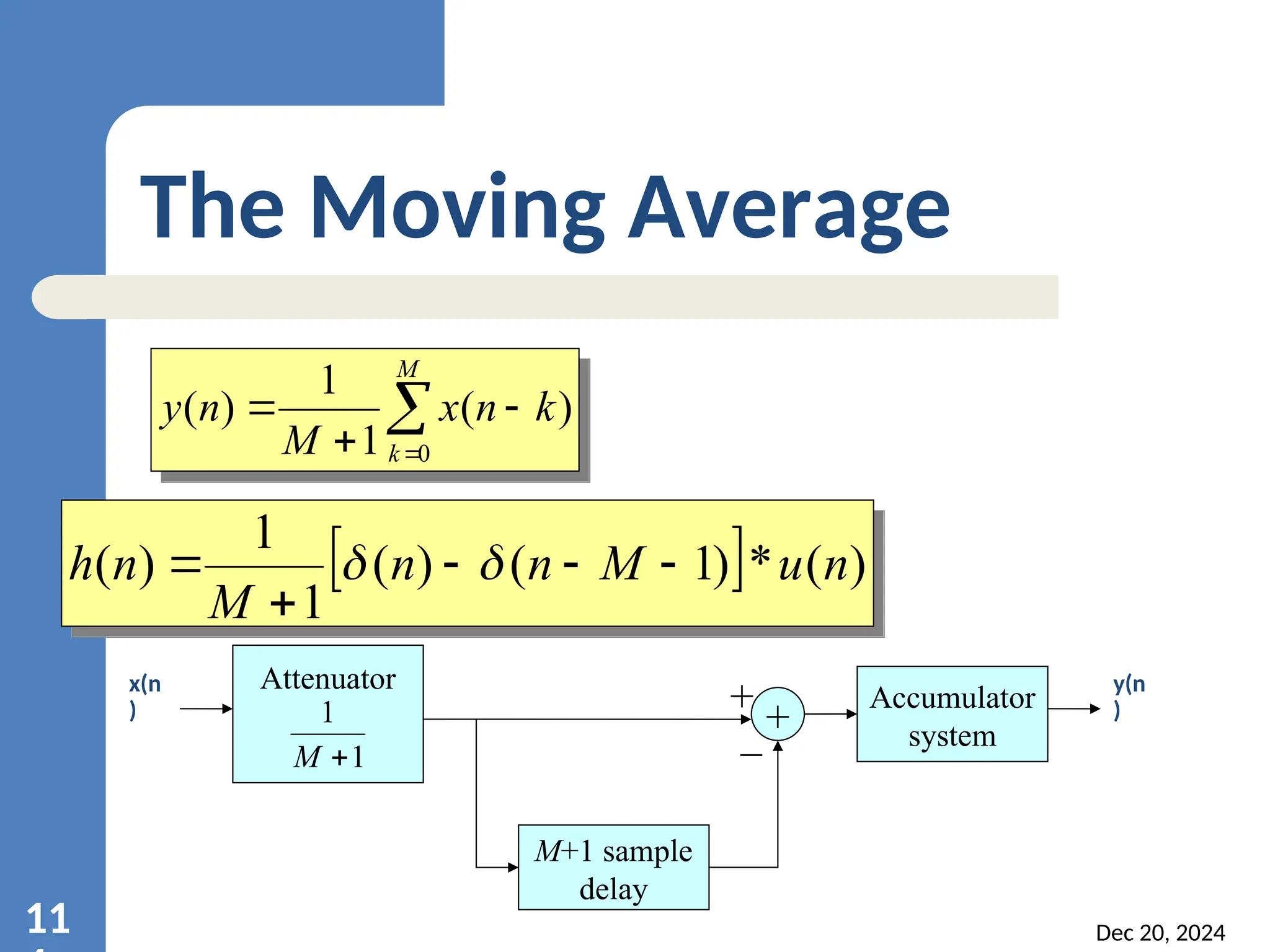
Dec 20, 2024 12 Moving Average      M k k n x M n y 0 ) ( 1 1 ) (      M k k n M n h 0 ) ( 1 1 ) (          k jk j e k h e H ) ( ) ( h(n) 0 0 M       M k jk e M 0 1 1                  j M j e e M 1 1 1 1 ) 1 (                          ) ( ) ( 1 1 2 / 2 / 2 / 2 / ) 1 ( 2 / ) 1 ( 2 / ) 1 ( j j j M j M j M j e e e e e e M                       ) ( ) ( 1 1 2 / 2 / 2 / ) 1 ( 2 / ) 1 ( 2 / j j M j M j M j e e e e e M                ) 2 / sin( ] 2 / ) 1 ( sin[ 1 1 2 / M e M M j n n

Dec 20, 2024 12 Moving Average                 ) 2 / sin( ] 2 / ) 1 ( sin[ 1 1 ) ( 2 / M e M e H M j j ) 2 / sin( ] 2 / ) 1 ( sin[ 1 1 | ) ( |       M M e H j

introduction to digital signal processing

More Related Content

What's hot

Similar to introduction to digital signal processing

Recently uploaded

introduction to digital signal processing