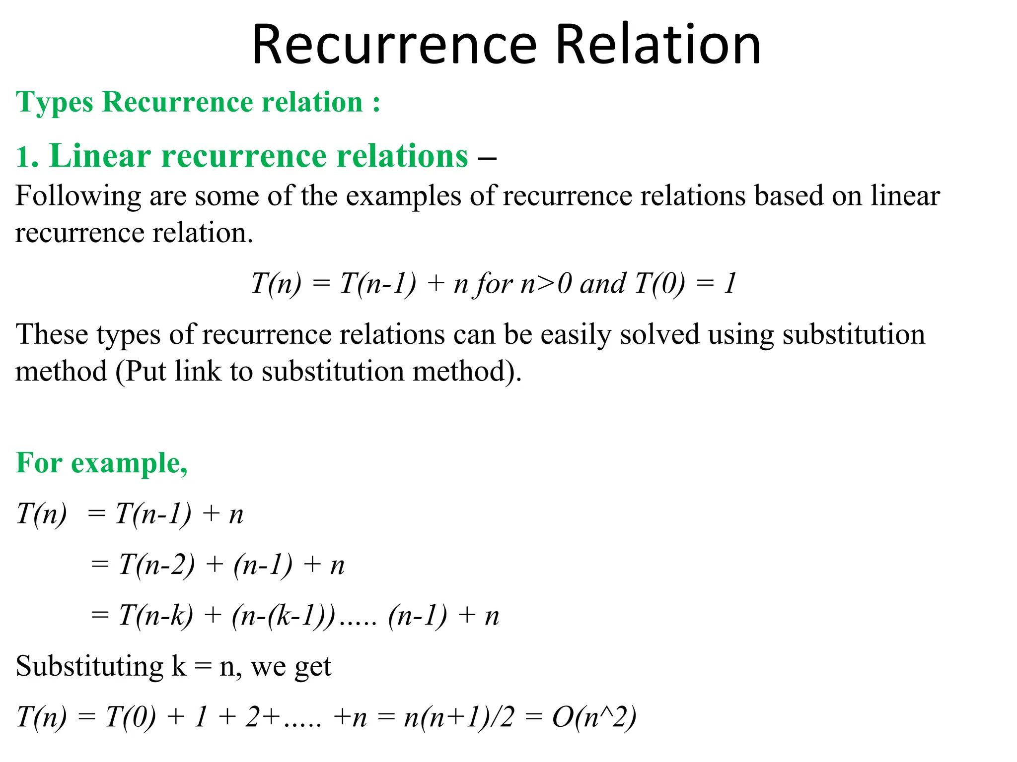
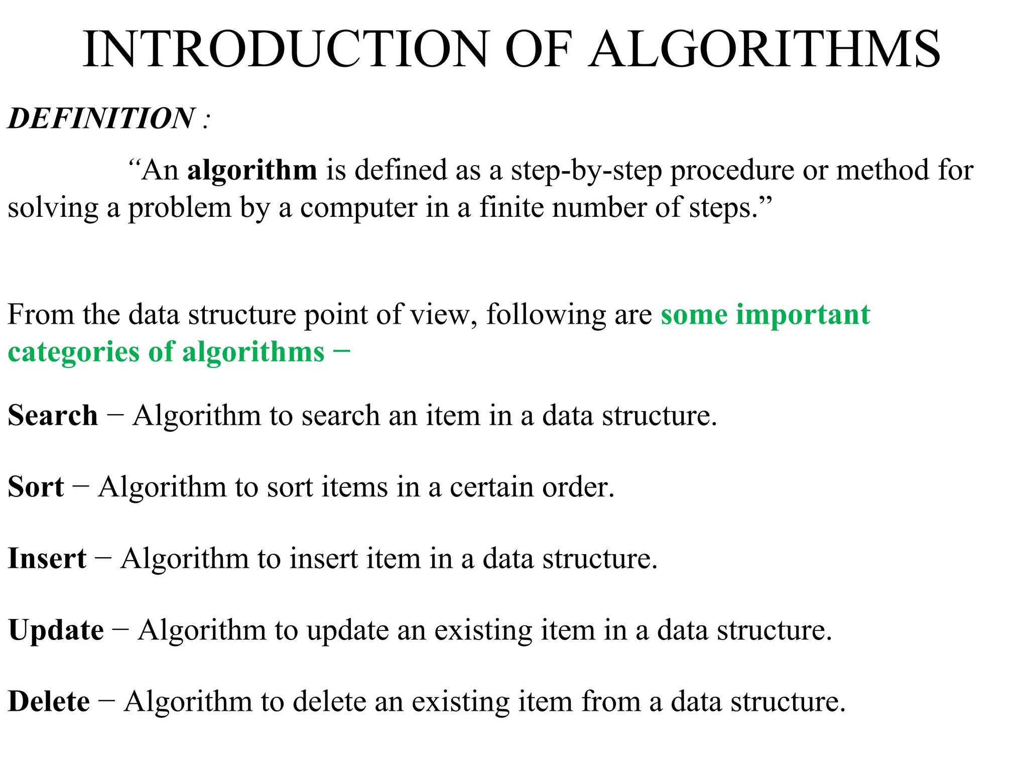
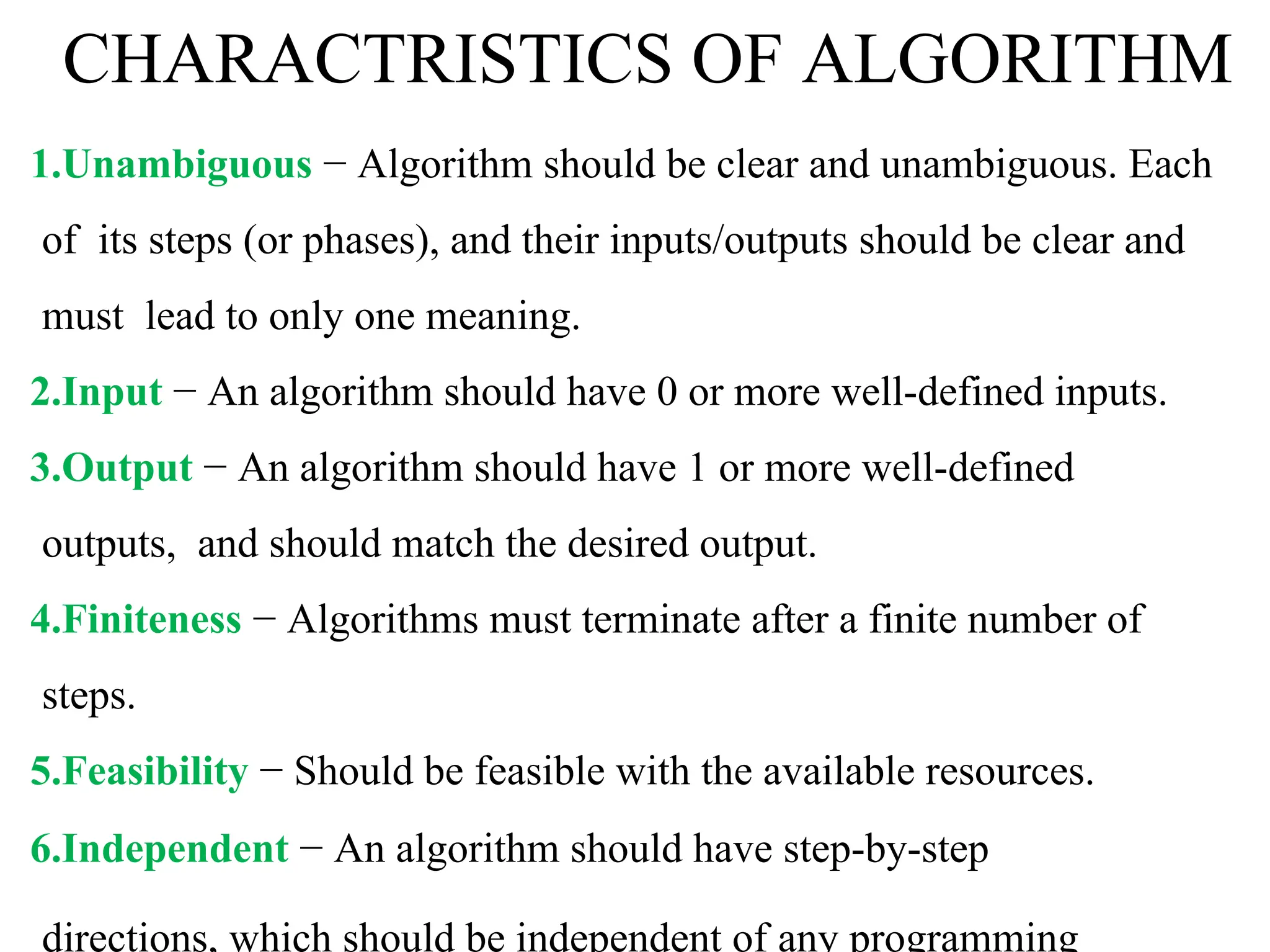
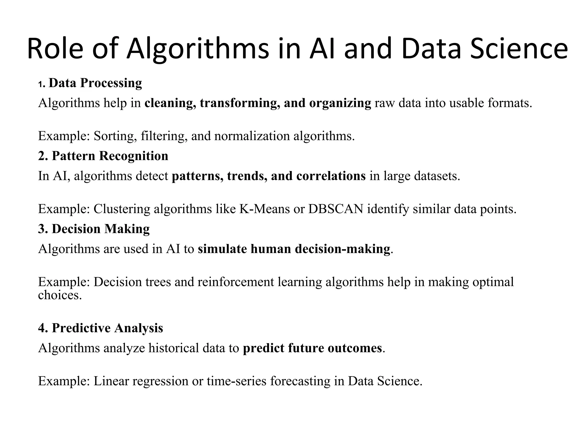
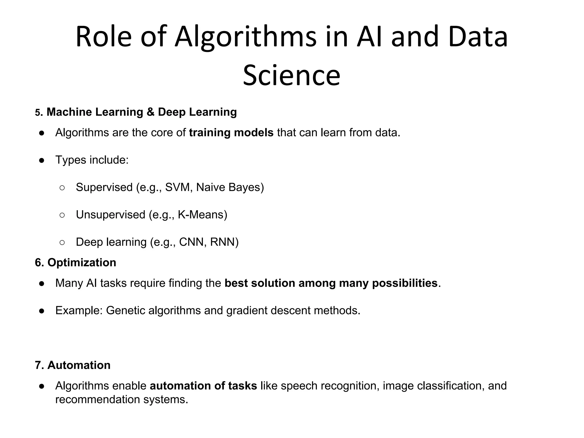
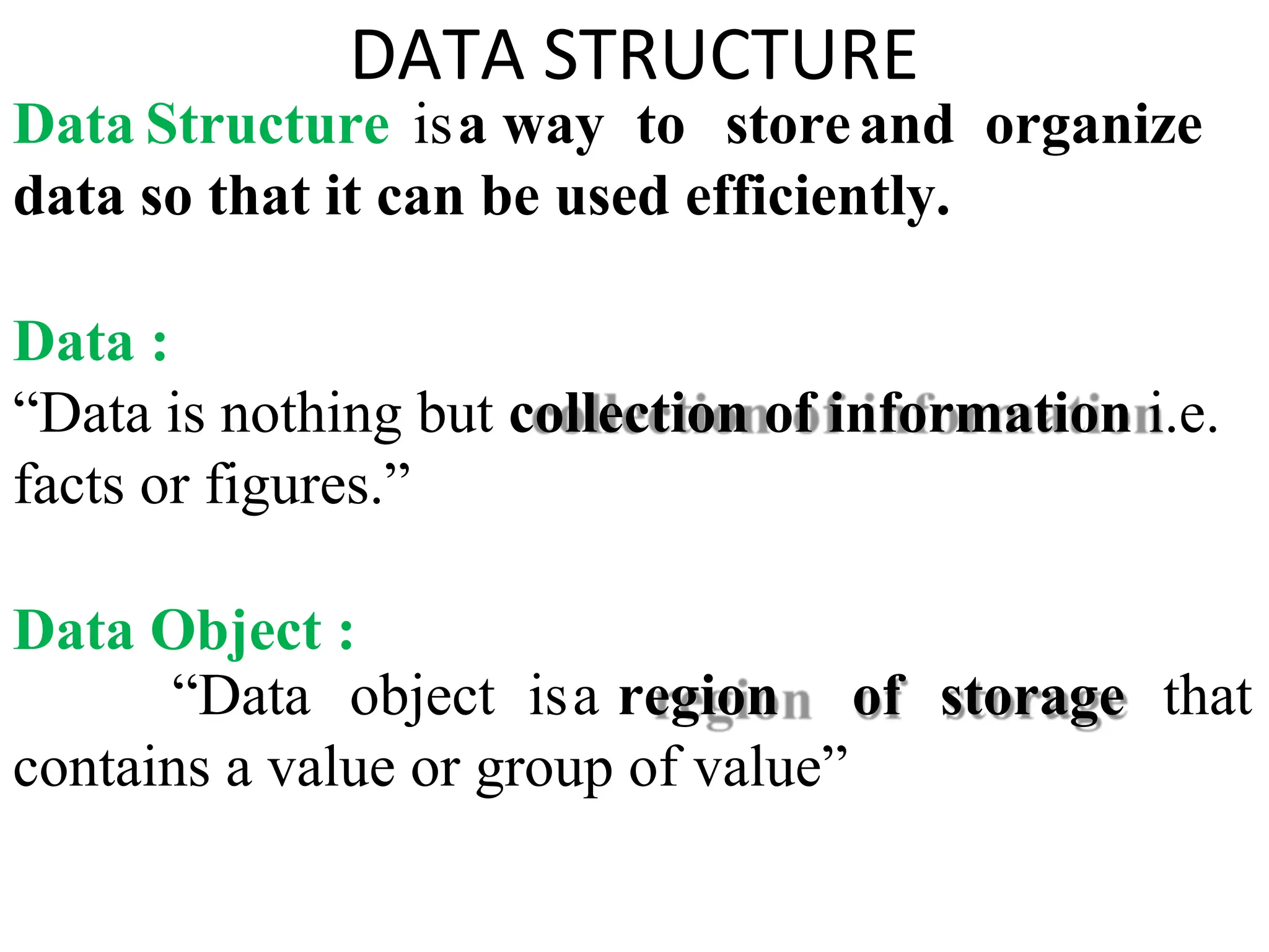
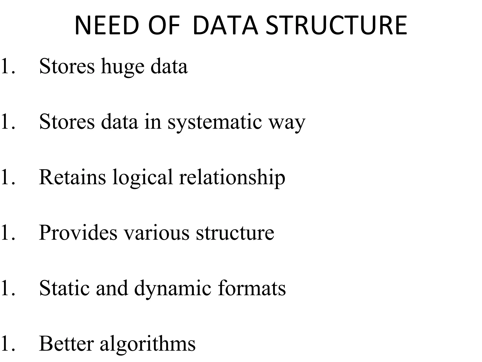
Introduction to data structure and algorithm

. “Introduction to Algorithm & Data Structure” .

Syllabus: • Introduction to Algorithm – Definition of Algorithm, Characteristics of Algorithm, Pseudocode and Flowcharts, Role of Algorithms in AI and Data Science. • Performance Analysis - Time and Space Complexity, Asymptotic Notations: Big-O, Big-Theta, Big-Omega, Best, Worst, and Average Case Analysis, Solving Recurrence Relations (Substitution and Iteration Methods) • Introduction to Data Structures: Concept of data, Data object, Data structure, Concept of Primitive and non-primitive, persistent and ephemeral data structures, Abstract Data Type(ADT) • Arrays -Array Operations (Traversal, Insertion, Deletion, Searching), Multidimensional Arrays • Linked Organization: Concept of linked organization, Singly Linked List, Doubly Linked List, Circular Linked List (Operations: Create, Display, Search, Insert) .

WHY TO LEARN DATA STRUCTURE??? •They enable efficient data manipulation, making it easier to preprocess and prepare data for modeling. •The choice of data structure often depends on the nature of the data and the ML model used. •Understanding data dimensions helps you grasp how your data evolves, improving feature engineering and model design.

Real -Time Applications of Data Structures Google Maps – Uses graphs to find the shortest path between locations. Web Browsers – Use stacks to manage back and forward navigation history. Social Media (Facebook) – Uses graphs to model user connections and hash maps for fast data retrieval. E-commerce Sites (Amazon) – Use trees for product categorization and tries for search suggestions. Operating Systems – Use queues for CPU/process scheduling and trees for file system structure. Databases (MySQL) – Use B-trees for indexing and fast query performance. Compilers – Use syntax trees and stacks for parsing and expression evaluation. AI & ML – Use matrices for neural networks and trees for decision-making. Messaging Apps (WhatsApp) – Use queues for managing real-time message delivery. Gaming (Pathfinding) – Use graphs and priority queues for AI movement and level navigation.

ALGORITHM – PROBLEM SOLVING Problem : “Problem is defined as situation or condition which needs to solve to achieve goal” Steps in Problem Solving : 1. Define the problem 2. Data gathering 3. Decide effective solution 4. Implement and evaluate the solution 5. Review the result.

PROBLEM SOLVING TECHNIQUES There are two types : 1. Algorithmic 2. Flowchart Algorithms is set of instructions which are written in simple english language. Flowchart is graphical representation of the algorithms.

Some other Problem Solving Techniques 1. Trial and error techniques 1. Divide and conquer techniques 1. Merging solution 1. The building block approach: The building-block approach is a method for building confidence in designs by working to develop understanding of behavior of lower-level components, then using the knowledge gained to inform representations of more complex assemblies. 5. Brainstorming techniques

INTRODUCTION OF ALGORITHMS DEFINITION : “An algorithm is defined as a step-by-step procedure or method for solving a problem by a computer in a finite number of steps.” From the data structure point of view, following are some important categories of algorithms − Search − Algorithm to search an item in a data structure. Sort − Algorithm to sort items in a certain order. Insert − Algorithm to insert item in a data structure. Update − Algorithm to update an existing item in a data structure. Delete − Algorithm to delete an existing item from a data structure.

CHARACTRISTICS OF ALGORITHM 1.Unambiguous − Algorithm should be clear and unambiguous. Each of its steps (or phases), and their inputs/outputs should be clear and must lead to only one meaning. 2.Input − An algorithm should have 0 or more well-defined inputs. 3.Output − An algorithm should have 1 or more well-defined outputs, and should match the desired output. 4.Finiteness − Algorithms must terminate after a finite number of steps. 5.Feasibility − Should be feasible with the available resources. 6.Independent − An algorithm should have step-by-step directions, which should be independent of any programming

Role of Algorithms in AI and Data Science 1. Data Processing Algorithms help in cleaning, transforming, and organizing raw data into usable formats. Example: Sorting, filtering, and normalization algorithms. 2. Pattern Recognition In AI, algorithms detect patterns, trends, and correlations in large datasets. Example: Clustering algorithms like K-Means or DBSCAN identify similar data points. 3. Decision Making Algorithms are used in AI to simulate human decision-making. Example: Decision trees and reinforcement learning algorithms help in making optimal choices. 4. Predictive Analysis Algorithms analyze historical data to predict future outcomes. Example: Linear regression or time-series forecasting in Data Science.

Role of Algorithms in AI and Data Science 5. Machine Learning & Deep Learning ● Algorithms are the core of training models that can learn from data. ● Types include: ○ Supervised (e.g., SVM, Naive Bayes) ○ Unsupervised (e.g., K-Means) ○ Deep learning (e.g., CNN, RNN) 6. Optimization ● Many AI tasks require finding the best solution among many possibilities. ● Example: Genetic algorithms and gradient descent methods. 7. Automation ● Algorithms enable automation of tasks like speech recognition, image classification, and recommendation systems.

EXAMPLE OF ALGORITHM Example Let's try to learn algorithm-writing by using an example. Problem − Design an algorithm to add two numbers and display the result. Step 1 − START Step 2 − declare three integers a, b & c Step 3 − define values of a & b Step 4 − add values of a & b Step 5 − store output of step 4 to c Step 6 − print c Step 7 − STOP

ALGORITHM DESIGN TOOL • There can be two tools : 1. Flowchart 2. Pseudo Code Flowchart : “ Flowchart is graphical representation of the algorithms” Pseudo Code : “It is simply an implementation of an algorithm in the form of annotations and informative text written in plain English.

FLOWCHART Symbols used in Flowchart:

Design an algorithm and flowchart to input fifty numbers and calculate their sum. Step 1: Start Step 2: Initialize the count variable to zero Step 3: Initialize the sum variable to zero Step 4: Read a number say x Step 5: Add 1 to the number in the count variable Step 6: Add the number x to the sum variable. Step 7: Is the count variable in the memory greater than 50? If yes, display the sum: go to step 8. If No, Repeat from step 4 Step8: Stop

WRITE A PROGRAM FOR ADDING 10 NUMBERS

WRITE A PROGRAM TO FIND FACTORIAL OF NUMBER

ALGORITHM ANALYSIS • A Priori Analysis − This is a theoretical analysis of an algorithm. Efficiency of an algorithm is measured by assuming that all other factors, for example, processor speed, are constant and have no effect on the implementation. • A Posterior Analysis − This is an empirical analysis of an algorithm. The selected algorithm is implemented using programming language. This is then executed on target computer machine. In this analysis, actual statistics like running time and space required, are collected.

CASES OFANALYSISALGORITHMS . There are 3 types 1. Worst case 2. Best case 3. Average case Best Case − Minimum time required for program execution. Average Case − Average time required for program execution. Worst Case − Maximum time required for program execution

Standard measure of efficiency There are two important complexity measures: 1. Time complexity 2. Space complexity Time complexity : “The time which is required for analysis of given problem of particular size is known as time complexity” Space complexity : “The amount of computer memory required to solve the given problem of particular size is called as space complexity” Time efficiency - a measure of amount of time for an algorithm to execute. Space efficiency - a measure of the amount of memory needed for an algorithm to execute.

ABSTRACT DATA TYPES ADT are like user defined data types which define operations on values using functions Without specifying what is there inside the function and how the operations are performed. e.g. stack ADT Stack contains elements of same type in sequential manner. Initialize(), push( ),pop(),isEmpty(),isFull()

Asymptotic notations Asymptotic Notations are languages that allow us to analyze an algorithm's running time by identifying its behavior as the input size for the algorithm increases. This is also known as an algorithm's growth rate Asymptotic Notation gives us the ability toanswer these questions. Following are the commonly used asymptotic notations to calculate the running time complexity of an algorithm. 1. Ο Notation 2. Ω Notation

n 5n2 6n 12 1 21.74% 26.09% 52.17% 10 87.41% 10.49% 2.09% 100 98.79% 1.19% 0.02% 1000 99.88% 0.12% 0.0002% Therefore, if the input size is n, then f(n) is a function of n that denotes the tim complexity. f(n) = 5n2 + 6n + 12 where n is the number of instructions executed, and it depends on the size of the input. When n=1 % of running time due to 5n2 = * 100 = 21.74% % of running time due to 6n = * 100 = 26.09% % of running time due to 12 = * 100 = 52.17% From the above calculation, it is observed that most of the time is taken by 12. But, we have to find the growth rate of f(n), we cannot say that the maximum amount of time is taken by 12. Let's assume the different values of n to find the growth rate of f(n).

• In mathematics, asymptotic analysis, also known as asymptotic, is a method of describing the limiting behavior of a function. • In computing, asymptotic analysis of an algorithm refers to defining the mathematical foundation of its run-time performance based on the input size. • For example, the running time of one operation is computed as f(n), and maybe for another operation, it is computed as g(n2 ). This means the first operation running time will increase linearly with the increase in n and the running time of the second operation will increase exponentially when n increases. Similarly, the running time of both operations will be nearly the same if n is small in value.

BIG – oh NOTATION Big Oh Notation, Ο The notation Ο(n) is the formal way to express the upper bound of an algorithm's running time. It measures the worst-case time complexity or the longest time an algorithm can take to complete.

Follow the steps below to calculate O for a program: • Break the program into smaller segments. • Find the number of operations performed for each segment (in terms of the input size) assuming the given input is such that the program takes the maximum time i.e. the worst-case scenario. • Add up all the operations and simplify it, let’s say it is f(n). • Remove all the constants and choose the term having the highest order because for n tends to infinitely the constants and the lower order terms in f(n) will be insignificant, let say the function is g(n) then, big oh notation is O(g(n)).

Omega NOTATION Omega Notation, Ω The notation Ω(n) is the formal way to express the lower bound of an algorithm's running time. It measures the best case time complexity or the best amount of time an algorithm can possibly take to comp

Follow the steps below to calculate Ω for a program: • Break the program into smaller segments. • Find the number of operations performed for each segment(in terms of the input size) assuming the given input is such that the program takes the least amount of time. • Add up all the operations and simplify it, let’s say it is f(n). • Remove all the constants and choose the term having the least order or any other function which is always less than f(n) when n tends to infinity, let say it is g(n) then, Omega (Ω) of f(n) is Ω(g(n)). • Omega notation doesn’t help to analyze an algorithm because it is bogus to evaluate an algorithm for the best cases of inputs. If there are positive constants n0 and c such that, to the right of n0 the f(n) always lies on or above c*g(n).

Theta NOTATION Theta Notation, θ The notation θ(n) is the formal way to express both the lower bound and the upper bound of an algorithm's running time. It is represented as follows −

Follow the steps below to calculate Θ for a program: • Break the program into smaller segments. • Find all types of inputs and calculate the number of operations they take to be executed. Make sure that the input cases are equally distributed. • Find the sum of all the calculated values and divide the sum by the total number of inputs let say the function of n obtained is g(n) after removing all the constants, then in Θ notation, it’s represented as Θ(g(n)). • Example: In a linear search problem let’s assume that all the cases are uniformly distributed (including the case when the key is absent in the array). So, sum all the cases when the key is present at positions 1, 2, 3, ……, n and not present, and divide the sum by n + 1.

DATA STRUCTURE Data Structure isa way to storeand organize data so that it can be used efficiently. Data : “Data is nothing but collection of information i.e. facts or figures.” Data Object : of storage that “Data object isa region contains a value or group of value”

NEED OF DATA STRUCTURE 1. Stores huge data 1. Stores data in systematic way 1. Retains logical relationship 1. Provides various structure 1. Static and dynamic formats 1. Better algorithms

ABSTRACT DATA TYPE ADT : “Abstract data types are mathematical models of a set of data values or information that share similar behavior or qualities and that can be specified and identified independent of specific implementations. Abstract data types, or ADTs, are typically used in algorithms.” Another definition of ADT is ADT is set of D, F and A. D – domain = Data object F – function = set of operations which can carried out on data object. A – axioms= Properties and rules of the operation

TYPES OFDATA STRUCTURE There are two types : 1. Primitives data structure 2. Non-primitive data structure

TYPES OFDATA STRUCTURE 1. Primitives data structure : “Primitive data structures are those which are predefined way of storing data by the system. ” e.g. int, char, float etc 2. Non-primitive data structure : “The data types that are derived from primary data types are known a non-Primitive data types. These datatype are used to store group of values.” e.g. struct, array, linklist, stack, tree , graph etc.

Linear and Non-Linear Data Structure 1. Linear Data Strucute : “Linear data structuretraverses the data elements sequentially, in which only one data element can directly be reached” Ex: Arrays, Linked Lists, stack, queue. 2. Non-Linear Data Strucute : “Every data item is attached to several other data items in a way that is specific for reflecting relationships.” Ex: Graph, Tree

Linear vs Non-Linear Data Structure

Static and Dynamic Data Structure 1. Static data strucure : “A static datastructureis anorganizationor collection of data in memory that is fixed in size.” Ex: Arrays 2. Dynamic Data Strucute : “ In Dynamic data structure the size of the structure in not fixed and can be modified during the operations performed on it” Ex: Linked list

Persistent and Ephemeral Data Structure 1. Persistent data strucure : “A persistent data structure is a data structure that always preserves the previous version of itself when it is modified..” Ex: Linked list, tree 2. Ephemeral Data Strucute : “ An ephemeral data structure is one of which only one version is available at a time(it does not preserve previous version).” Ex: RAM , Cache memory

Relationship among Data, Data Structure and Algorithms Data is considered as set of facts and figures or data is value of group of value which is in particular format. Data structure is method of gathering as well as organizing data in such manner that several operation can be performed Problem is definedas a situation or condition which needto solve to achieve the goals Algorithm is set of ordered instruction which are written in simple english language.

ALGORITHMIC STRATEGIES Algorithm design strategies are the generalapproaches used to develop efficient solution to problem. Algorithm Strategies are : 1. Divide and conquer 2. Merge sort 3. Recursive algorithm 4. Backtracking algorithms 5. Heuristic algorithms 6. Dynamic Programming algorithm

DIVIDE AND CONQUER In divide and conquer approach, the problem in hand, is divided into smaller sub-problems and then each problem is solved independently. When we keep on dividing the subproblems into even smaller sub- problems, we may eventually reach a stage where no more division is possible. Those "atomic" smallest possible sub-problem (fractions) are solved. The solution of all sub-problems is finally merged in order to obtain the solution of an original problem.

DIVIDE AND CONQUER Operation for strategy : Divide – Break the problem into subproblem of same type Conquer – Recursively solve these sub problem Combine – Combine the solution of sub problem are based on divide and conquer Following algorithms strategies : 1. Merge sort 2. Binary search 3. Quick sort 4. Closest pair 5. Tower of Hanoi

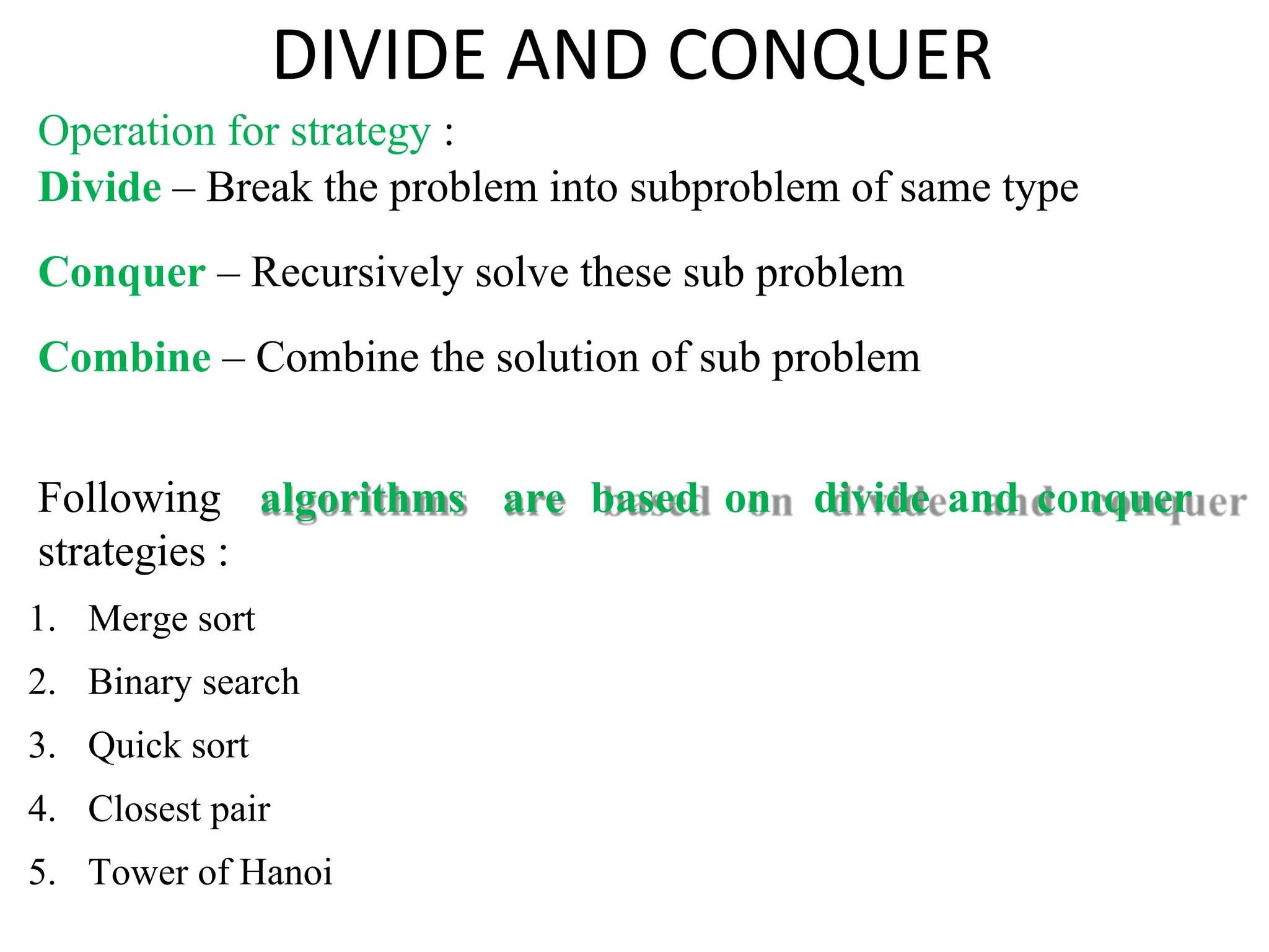
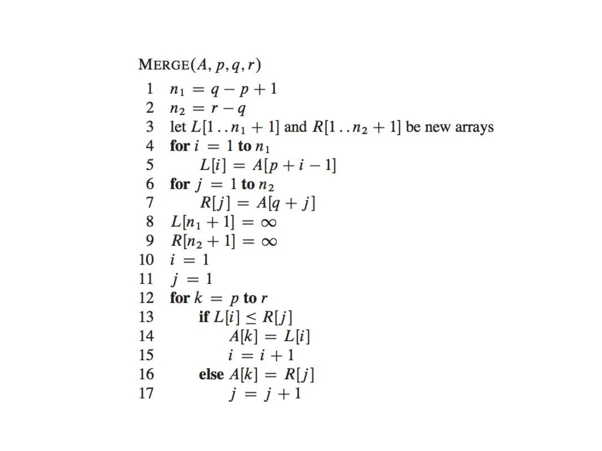
DIVIDE AND CONQUER 1. Merge sort : Merge Sort is a divide-and-conquer algorithm. It divides the input array in two halves, calls itself for the two halves and then merges the two sorted halves. The merge() function is used for merging two halves. The merge(arr, l, m, r) is key process that assumes that arr[l..m] and arr[m+1..r] are sorted and merges the two sorted sub-arrays into one.

DIVIDE AND CONQUER 2. Tower of Hanoi : Tower of Hanoi is a mathematical puzzle where we have three rods and n disks. The objective of the puzzle is to move the entire stack to another rod, obeying the following simple rules: 1) Only one disk can be moved at a time. 2)Each move consists of taking the upper disk from one of the stacks and placing it on top of another stack i.e. a disk can only be moved if it is the uppermost disk on a stack. 1) No disk may be placed on top of a smaller disk.

DIVIDE AND CONQUER 2. Tower of Hanoi : Example

GREEDY STRATEGIES Greedy algorithm : An algorithm is designed to achieve optimum solution for a given problem. In greedy algorithm approach, decisions are made from the given solution domain. As being greedy, the closest solution that seems to provide an optimum solution is chosen. Example of greedy strategy : 1. Travelling Salesman Problem 2. Prim's Minimal Spanning Tree Algorithm 3. Kruskal's Minimal Spanning Tree Algorithm 4. Dijkstra's Minimal Spanning Tree Algorithm 5. Knapsack Problem 6. Job Scheduling Problem

GREEDY STRATEGIES 1. Minimum Spanning tree (Prims or Kruskal’s algorithms) The cost of the spanning tree is the sum of the weights of all the edges in the tree. There can be many spanning trees. Minimum spanning tree is the spanning tree where the cost is minimum among all the spanning trees. There also can be many minimum spanning trees.

GREEDY STRATEGIES 2. Kruskal’s algorithms : Kruskal’s Algorithm builds the spanning tree by adding edges one by one into a growing spanning tree. Kruskal's algorithm follows greedy approach as in each iteration it finds an edge which has least weight and add it to the growing spanning tree. Algorithm Steps : Sort the graph edges with respect to their weights. Start adding edgesto the MST from the edge with the smallest weight until the edge of the largest weight. Only add edgeswhich doesn't form a cycle , edgeswhich connect only disconnected components.

GREEDY STRATEGIES 2. Kruskal’s algorithms : Example .

GREEDY STRATEGIES 2. Prims algorithm: Prim’s Algorithm also use Greedy approach to find the minimum spanning tree. In Prim’s Algorithm we grow the spanning tree from a starting position. Unlike an edge in Kruskal's, we add vertex to the growing spanning tree in Prim's. Algorithm Steps: 1. Initialize the minimum spanning tree with a vertex chosen at random. 2.Find all the edges that connect the tree to new vertices, find the minimum and add it to the tree. 1. Keep repeating step 2 until we get a minimum spanning tree.

GREEDYSTRATEGIES 2. Prims algorithm: Example

The step Count method for time complexity The step Count method is also called as Frequency Count method. • step count for different statements: 1. Comments: • Comments are used for giving extra meaning to the program. They are not executed during the execution. Comments are ignored during execution. • Therefore the number of times that a comment executes is 0. 2. Conditional statements: • Conditional statements check the condition and if the condition is correct then the conditional subpart will be executed. So the execution of conditional statements happens only once. The compiler will execute the conditional statements to check whether the condition is correct or not so it will be executed one time. • In if-else statements the if statement is executed one time but the else statement will be executed zero or one time because if the “if” statement is executed then the else statement will not execute.

• In switch case statements the starting switch(condition) statement will be executed one time but the inner case statements will execute if none of the previous case statements are executed. • In nested if and if else ladder statements also the initial if statement is executed at least once but inner statements will be executed based on the previous statements’ execution. 3. Loop statements: • Loop statements are iterative statements. They are executed one or more times based on a given condition. • A typical for(i = 0; i ≤ n; i++) statement will be executed “n+1” times for the first n times the condition is satisfied and the inner loop will be executed and for the (n+1)th time the condition is failed and the loop terminates.

• While: The statement is executed until the given condition is satisfied. • Do while: The statement will repeat until the given condition is satisfied. The do-while statement will execute at least once because for the first time it will not check the condition. 4. Functions: • Functions are executed based on the number of times they get called. If they get called n times they will be executed n times. If they are not called at least once then they will not be executed. Other statements like BEGIN, END and goto statements will be executed one time.

switch(expression) • { • case value1: statement_1; • break; • case value2: statement_2; • break; • . • . • . • case value_n: statement_n; • break; • default: default_statement; • } if (condition1) { // Executes when condition1 is true if (condition2) { // Executes when condition2 is true } else { // Executes when condition2 is false }

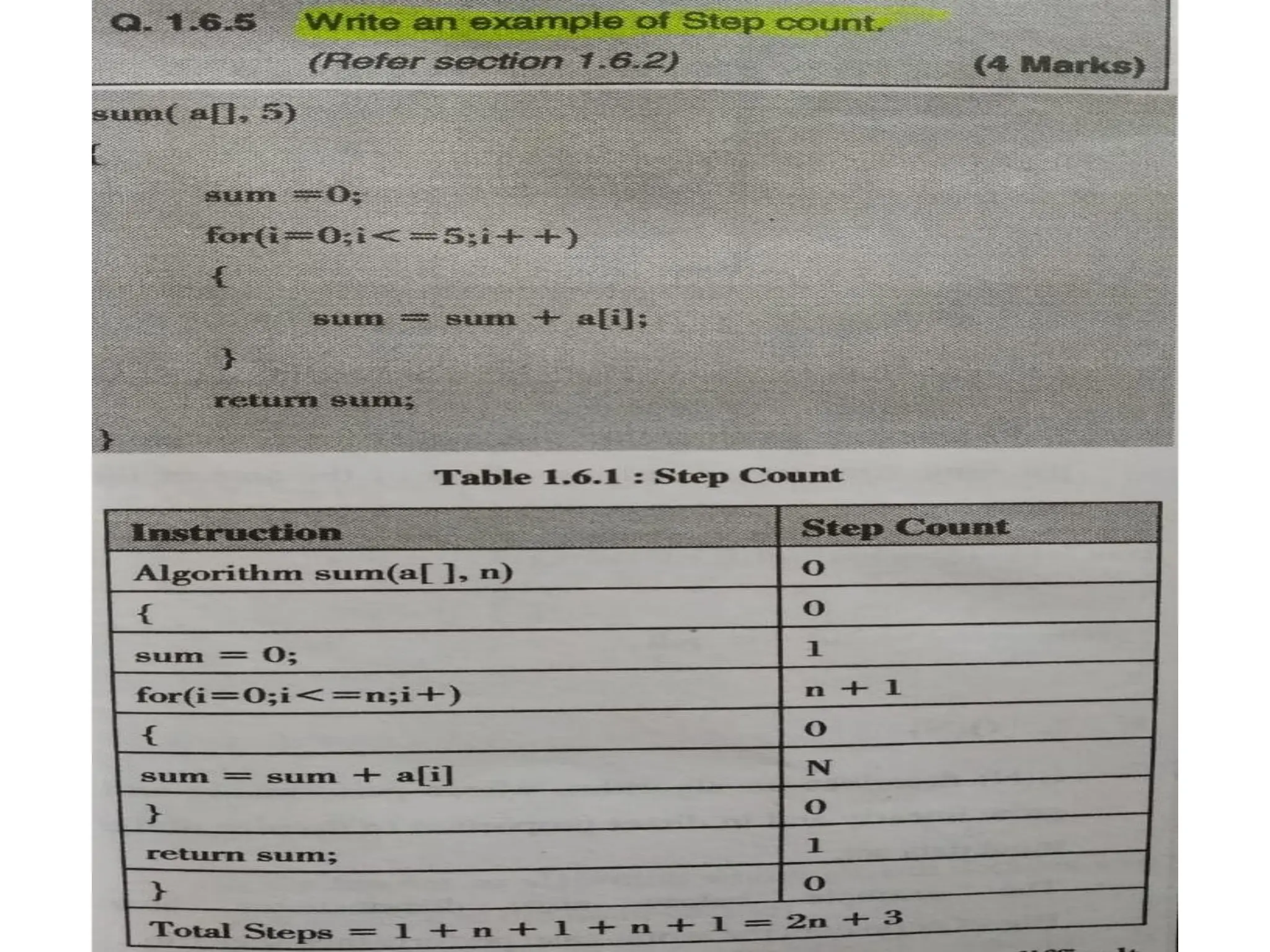
Analysis of Linear Search algorithm Let us consider a Linear Search Algorithm. Linearsearch(arr, n, key) { i = 0; for(i = 0; i < n; i++) { if(arr[i] == key) { printf(“Found”); } }

Where, i = 0, is an initialization statement and takes O(1) times. for(i = 0;i < n ; i++), is a loop and it takes O(n+1) times . if(arr[i] == key), is a conditional statement and takes O(1) times. printf(“Found”), is a function and that takes O(0)/O(1) times. Therefore Total Number of times it is executed is n + 4 times. As we ignore lower exponents in time complexity total time became O(n). Time complexity: O(n).

Simple Examples #include <iostream> using namespace std; int main() { int i, n = 8; for (i = 1; i <= n; i++) { cout << "Hello World !!!n"; } return 0; } # time complexity O(n)

• #include <iostream> • using namespace std; • int main() • { • int i, n = 8; • for (i = 1; i <= n; i=i*2) • { • cout << "Hello World !!!n"; • } • return 0; • } #time complexity O(log2 (n))

• #include <iostream> • #include <cmath> • using namespace std; • int main() • { • int i, n = 8; • for (i = 2; i <= n; i=pow(i,2)) • { • cout << "Hello World !!!n"; • } • return 0; } # time complexity O(log(log n))

Recurrence Relation Recurrence relation : “A recurrence relation is an equationthat recursively defines a sequence where the next term is a function of the previousterms (Expressing FnFn as some combination of FiFi with i<ni<n).” Example − Fibonacci series − Fn=Fn−1+Fn−2 .

Recurrence Relation Types Recurrence relation : 1. Linear recurrence relations – Following are some of the examples of recurrence relations based on linear recurrence relation. T(n) = T(n-1) + n for n>0 and T(0) = 1 These types of recurrence relations can be easily solved using substitution method (Put link to substitution method). For example, T(n) = T(n-1) + n = T(n-2) + (n-1) + n = T(n-k) + (n-(k-1))….. (n-1) + n Substituting k = n, we get T(n) = T(0) + 1 + 2+….. +n = n(n+1)/2 = O(n^2)

Recurrence Relation Types Recurrence relation : 1. Homogeneous linear recurrence relation – Homogeneous refers to the fact that the total degree of each term is the same (thus there is no constant term) Constant Coefficients refers to the fact that c1,c2,...,ck are fixed real numbers that do not depend on n. ... The recurrence relation An = (1.04)An−1 is a linear homogeneous recurrence relation of degree one. .

Type of Recurrence Relation Generating Functions Generating Functions represents sequences whereeach term of a sequence is expressed as a coefficient of a variable x in a formal power series. Mathematically, for an infinite sequence, say a0,a1,a2,…,ak,…,a0,a1,a2,…,ak,…, the generating function will be − Gx=a0 +a1 x+a2 x2 +⋯+ak xk +⋯=∑ak xk Some Areas of Application Generating functions can be used for the following purposes − -For solving a variety of counting problems. For example, the number of ways to make change for a Rs. 100 note with the notes of denominations Rs.1, Rs.2, Rs.5, Rs.10, Rs.20 and Rs.50 -For solving recurrence relations -For proving some of the combinatorial identities -For finding asymptotic formulae for terms of sequences .

Introduction to data structure and algorithm

More Related Content

Similar to Introduction to data structure and algorithm

Recently uploaded

Introduction to data structure and algorithm