Introduction to Computational Mathematics (2nd Edition, 2015)

October 29, 2014 11:19 BC: 9404 – Intro to Comp Maths 2nd Ed. Yang-Comp-Maths2014 page v Preface Computational mathematics is essentially the foundation of modern scientific computing. Traditional ways of doing sciences consist of two major paradigms: by theory and by experiment. With the steady increase in computer power, there emerges a third paradigm of doing sciences: by computer simulation. Numerical algorithms are the very essence of any computer simulation, and computational mathematics is just the science of developing and analyzing numerical algorithms. The science that studies numerical algorithms is numerical analysis or more broadly computational mathematics. Loosely speaking, numerical algorithms and analysis should include four categories of algorithms: numerical linear algebra, numerical optimization, numerical solutions of differential equations (ODEs and PDEs) and stochastic data modelling. Many numerical algorithms were developed well before the computer was invented. For example, Newton’s method for finding roots of nonlinear equations was developed in 1669, and Gauss quadrature for numerical integration was formulated in 1814. However, their true power and efficiency have been demonstrated again and again in modern scientific computing. Since the invention of the modern computer in the 1940s, many numerical algorithms have been developed since the 1950s. As the speed of com- puters increases, together with the increase in the efficiency of numerical algorithms, a diverse range of complex and challenging problems in mathematics, science and engineering can nowadays be solved numerically to very high accuracy. Numerical algorithms have become more important than ever. The topics of computational mathematics are broad and the related literature is vast. It is often a daunting task for beginners to find the right book(s) and to learn the right algorithms that are widely used in v

November 3, 2014 11:34 BC: 9404 – Intro to Comp Maths 2nd Ed. Yang-Comp-Maths2014 page vi vi Introduction to Computational Mathematics computational mathematics. Even for lecturers and educators, it is no trivial task to decide what algorithms to teach and to provide balanced coverage of a wide range of topics, because there are so many algorithms to choose from. The first edition of this book was published by World Scientific Publish- ing in 2008 and it was well received. Many universities courses used it as a main reference. Constructive feedbacks and helpful comments have also been received from the readers. This second edition has incorporated all these comments and consequently includes more algorithms and new algorithms to reflect the state-of-the-art developments such as computational intelligence and swarm intelligence. Therefore, this new edition strives to provide extensive coverage of efficient algorithms commonly used in computational mathematics and modern scientific computing. It covers all the major topics including root-finding algorithms, numerical integration, interpolation, linear algebra, eigenvalues, numerical methods of ordinary differential equations (ODEs) and partial differential equations (PDEs), finite difference methods, finite element methods, finite volume methods, algorithm complexity, optimization, mathematical programming, stochastic models such as least squares and regression, machine learning such as neural networks and support vector machine, computational intelligence and swarm intelligence such as cuckoo search, bat algorithm, firefly algorithm as well as particle swarm optimization. The book covers both traditional methods and new algorithms with dozens of worked examples to demonstrate how these algorithms work. Thus, this book can be used as a textbook and/or reference book, especially suitable for undergraduates and graduates in computational mathematics, engineering, computer science, computational intelligence, data science and scientific computing. Xin-She Yang London, 2014

October 29, 2014 11:19 BC: 9404 – Intro to Comp Maths 2nd Ed. Yang-Comp-Maths2014 page vii Contents Preface v I Mathematical Foundations 1 1. Mathematical Foundations 3 1.1 The Essence of an Algorithm . . . . . . . . . . . . . . . . 3 1.2 Big-O Notations . . . . . . . . . . . . . . . . . . . . . . . 5 1.3 Diﬀerentiation and Integration . . . . . . . . . . . . . . . 6 1.4 Vector and Vector Calculus . . . . . . . . . . . . . . . . . 10 1.5 Matrices and Matrix Decomposition . . . . . . . . . . . . 15 1.6 Determinant and Inverse . . . . . . . . . . . . . . . . . . . 20 1.7 Matrix Exponential . . . . . . . . . . . . . . . . . . . . . . 24 1.8 Hermitian and Quadratic Forms . . . . . . . . . . . . . . . 26 1.9 Eigenvalues and Eigenvectors . . . . . . . . . . . . . . . . 28 1.10 Deﬁniteness of Matrices . . . . . . . . . . . . . . . . . . . 31 2. Algorithmic Complexity, Norms and Convexity 33 2.1 Computational Complexity . . . . . . . . . . . . . . . . . 33 2.2 NP-Complete Problems . . . . . . . . . . . . . . . . . . . 34 2.3 Vector and Matrix Norms . . . . . . . . . . . . . . . . . . 35 2.4 Distribution of Eigenvalues . . . . . . . . . . . . . . . . . 37 2.5 Spectral Radius of Matrices . . . . . . . . . . . . . . . . . 44 2.6 Hessian Matrix . . . . . . . . . . . . . . . . . . . . . . . . 47 2.7 Convexity . . . . . . . . . . . . . . . . . . . . . . . . . . . 48 vii

October 29, 2014 11:19 BC: 9404 – Intro to Comp Maths 2nd Ed. Yang-Comp-Maths2014 page viii viii Introduction to Computational Mathematics 3. Ordinary Differential Equations 51 3.1 Ordinary Differential Equations . . . . . . . . . . . . . . . 51 3.2 First-Order ODEs . . . . . . . . . . . . . . . . . . . . . . 52 3.3 Higher-Order ODEs . . . . . . . . . . . . . . . . . . . . . 53 3.4 Linear System . . . . . . . . . . . . . . . . . . . . . . . . . 56 3.5 Sturm-Liouville Equation . . . . . . . . . . . . . . . . . . 58 4. Partial Differential Equations 59 4.1 Partial Differential Equations . . . . . . . . . . . . . . . . 59 4.1.1 First-Order Partial Differential Equation . . . . . 60 4.1.2 Classification of Second-Order Equations . . . . . 61 4.2 Mathematical Models . . . . . . . . . . . . . . . . . . . . . 61 4.2.1 Parabolic Equation . . . . . . . . . . . . . . . . . 61 4.2.2 Poisson’s Equation . . . . . . . . . . . . . . . . . . 61 4.2.3 Wave Equation . . . . . . . . . . . . . . . . . . . . 62 4.3 Solution Techniques . . . . . . . . . . . . . . . . . . . . . 64 4.3.1 Separation of Variables . . . . . . . . . . . . . . . 65 4.3.2 Laplace Transform . . . . . . . . . . . . . . . . . . 67 4.3.3 Similarity Solution . . . . . . . . . . . . . . . . . . 68 II Numerical Algorithms 71 5. Roots of Nonlinear Equations 73 5.1 Bisection Method . . . . . . . . . . . . . . . . . . . . . . . 73 5.2 Simple Iterations . . . . . . . . . . . . . . . . . . . . . . . 75 5.3 Newton’s Method . . . . . . . . . . . . . . . . . . . . . . . 76 5.4 Iteration Methods . . . . . . . . . . . . . . . . . . . . . . . 78 5.5 Numerical Oscillations and Chaos . . . . . . . . . . . . . . 81 6. Numerical Integration 85 6.1 Trapezium Rule . . . . . . . . . . . . . . . . . . . . . . . . 86 6.2 Simpson’s Rule . . . . . . . . . . . . . . . . . . . . . . . . 87 6.3 Gaussian Integration . . . . . . . . . . . . . . . . . . . . . 89 7. Computational Linear Algebra 95 7.1 System of Linear Equations . . . . . . . . . . . . . . . . . 95 7.2 Gauss Elimination . . . . . . . . . . . . . . . . . . . . . . 97

October 29, 2014 11:19 BC: 9404 – Intro to Comp Maths 2nd Ed. Yang-Comp-Maths2014 page ix Contents ix 7.3 LU Factorization . . . . . . . . . . . . . . . . . . . . . . . 101 7.4 Iteration Methods . . . . . . . . . . . . . . . . . . . . . . . 103 7.4.1 Jacobi Iteration Method . . . . . . . . . . . . . . . 103 7.4.2 Gauss-Seidel Iteration . . . . . . . . . . . . . . . . 107 7.4.3 Relaxation Method . . . . . . . . . . . . . . . . . 108 7.5 Newton-Raphson Method . . . . . . . . . . . . . . . . . . 109 7.6 QR Decomposition . . . . . . . . . . . . . . . . . . . . . . 110 7.7 Conjugate Gradient Method . . . . . . . . . . . . . . . . . 115 8. Interpolation 117 8.1 Spline Interpolation . . . . . . . . . . . . . . . . . . . . . . 117 8.1.1 Linear Spline Functions . . . . . . . . . . . . . . . 117 8.1.2 Cubic Spline Functions . . . . . . . . . . . . . . . 118 8.2 Lagrange Interpolating Polynomials . . . . . . . . . . . . . 123 8.3 Bézier Curve . . . . . . . . . . . . . . . . . . . . . . . . . 125 III Numerical Methods of PDEs 127 9. Finite Difference Methods for ODEs 129 9.1 Integration of ODEs . . . . . . . . . . . . . . . . . . . . . 129 9.2 Euler Scheme . . . . . . . . . . . . . . . . . . . . . . . . . 130 9.3 Leap-Frog Method . . . . . . . . . . . . . . . . . . . . . . 131 9.4 Runge-Kutta Method . . . . . . . . . . . . . . . . . . . . . 132 9.5 Shooting Methods . . . . . . . . . . . . . . . . . . . . . . 134 10. Finite Difference Methods for PDEs 139 10.1 Hyperbolic Equations . . . . . . . . . . . . . . . . . . . . . 139 10.2 Parabolic Equation . . . . . . . . . . . . . . . . . . . . . . 142 10.3 Elliptical Equation . . . . . . . . . . . . . . . . . . . . . . 143 10.4 Spectral Methods . . . . . . . . . . . . . . . . . . . . . . . 146 10.5 Pattern Formation . . . . . . . . . . . . . . . . . . . . . . 148 10.6 Cellular Automata . . . . . . . . . . . . . . . . . . . . . . 150 11. Finite Volume Method 153 11.1 Concept of the Finite Volume . . . . . . . . . . . . . . . . 153 11.2 Elliptic Equations . . . . . . . . . . . . . . . . . . . . . . . 154 11.3 Parabolic Equations . . . . . . . . . . . . . . . . . . . . . 155 11.4 Hyperbolic Equations . . . . . . . . . . . . . . . . . . . . . 156

October 29, 2014 11:19 BC: 9404 – Intro to Comp Maths 2nd Ed. Yang-Comp-Maths2014 page x x Introduction to Computational Mathematics 12. Finite Element Method 157 12.1 Finite Element Formulation . . . . . . . . . . . . . . . . . 157 12.1.1 Weak Formulation . . . . . . . . . . . . . . . . . . 157 12.1.2 Galerkin Method . . . . . . . . . . . . . . . . . . . 158 12.1.3 Shape Functions . . . . . . . . . . . . . . . . . . . 159 12.2 Derivatives and Integration . . . . . . . . . . . . . . . . . 163 12.2.1 Derivatives . . . . . . . . . . . . . . . . . . . . . . 163 12.2.2 Gauss Quadrature . . . . . . . . . . . . . . . . . . 164 12.3 Poisson’s Equation . . . . . . . . . . . . . . . . . . . . . . 165 12.4 Transient Problems . . . . . . . . . . . . . . . . . . . . . . 169 IV Mathematical Programming 171 13. Mathematical Optimization 173 13.1 Optimization . . . . . . . . . . . . . . . . . . . . . . . . . 173 13.2 Optimality Criteria . . . . . . . . . . . . . . . . . . . . . . 175 13.3 Unconstrained Optimization . . . . . . . . . . . . . . . . . 177 13.3.1 Univariate Functions . . . . . . . . . . . . . . . . 177 13.3.2 Multivariate Functions . . . . . . . . . . . . . . . 178 13.4 Gradient-Based Methods . . . . . . . . . . . . . . . . . . . 180 13.4.1 Newton’s Method . . . . . . . . . . . . . . . . . . 181 13.4.2 Steepest Descent Method . . . . . . . . . . . . . . 182 14. Mathematical Programming 187 14.1 Linear Programming . . . . . . . . . . . . . . . . . . . . . 187 14.2 Simplex Method . . . . . . . . . . . . . . . . . . . . . . . 189 14.2.1 Basic Procedure . . . . . . . . . . . . . . . . . . . 189 14.2.2 Augmented Form . . . . . . . . . . . . . . . . . . 191 14.2.3 A Case Study . . . . . . . . . . . . . . . . . . . . 192 14.3 Nonlinear Programming . . . . . . . . . . . . . . . . . . . 196 14.4 Penalty Method . . . . . . . . . . . . . . . . . . . . . . . . 196 14.5 Lagrange Multipliers . . . . . . . . . . . . . . . . . . . . . 197 14.6 Karush-Kuhn-Tucker Conditions . . . . . . . . . . . . . . 199 14.7 Sequential Quadratic Programming . . . . . . . . . . . . . 200 14.7.1 Quadratic Programming . . . . . . . . . . . . . . 200 14.7.2 Sequential Quadratic Programming . . . . . . . . 200 14.8 No Free Lunch Theorems . . . . . . . . . . . . . . . . . . 202

October 29, 2014 11:19 BC: 9404 – Intro to Comp Maths 2nd Ed. Yang-Comp-Maths2014 page xi Contents xi V Stochastic Methods and Data Modelling 205 15. Stochastic Models 207 15.1 Random Variables . . . . . . . . . . . . . . . . . . . . . . 207 15.2 Binomial and Poisson Distributions . . . . . . . . . . . . . 209 15.3 Gaussian Distribution . . . . . . . . . . . . . . . . . . . . 211 15.4 Other Distributions . . . . . . . . . . . . . . . . . . . . . . 213 15.5 The Central Limit Theorem . . . . . . . . . . . . . . . . . 215 15.6 Weibull Distribution . . . . . . . . . . . . . . . . . . . . . 216 16. Data Modelling 221 16.1 Sample Mean and Variance . . . . . . . . . . . . . . . . . 221 16.2 Method of Least Squares . . . . . . . . . . . . . . . . . . . 223 16.2.1 Maximum Likelihood . . . . . . . . . . . . . . . . 223 16.2.2 Linear Regression . . . . . . . . . . . . . . . . . . 223 16.3 Correlation Coefficient . . . . . . . . . . . . . . . . . . . . 226 16.4 Linearization . . . . . . . . . . . . . . . . . . . . . . . . . 227 16.5 Generalized Linear Regression . . . . . . . . . . . . . . . . 229 16.6 Nonlinear Regression . . . . . . . . . . . . . . . . . . . . . 233 16.7 Hypothesis Testing . . . . . . . . . . . . . . . . . . . . . . 237 16.7.1 Confidence Interval . . . . . . . . . . . . . . . . . 237 16.7.2 Student’s t-Distribution . . . . . . . . . . . . . . . 238 16.7.3 Student’s t-Test . . . . . . . . . . . . . . . . . . . 240 17. Data Mining, Neural Networks and Support Vector Machine 243 17.1 Clustering Methods . . . . . . . . . . . . . . . . . . . . . . 243 17.1.1 Hierarchy Clustering . . . . . . . . . . . . . . . . . 243 17.1.2 k-Means Clustering Method . . . . . . . . . . . . 244 17.2 Artificial Neural Networks . . . . . . . . . . . . . . . . . . 247 17.2.1 Artificial Neuron . . . . . . . . . . . . . . . . . . . 247 17.2.2 Artificial Neural Networks . . . . . . . . . . . . . 248 17.2.3 Back Propagation Algorithm . . . . . . . . . . . . 250 17.3 Support Vector Machine . . . . . . . . . . . . . . . . . . . 251 17.3.1 Classifications . . . . . . . . . . . . . . . . . . . . 251 17.3.2 Statistical Learning Theory . . . . . . . . . . . . . 252 17.3.3 Linear Support Vector Machine . . . . . . . . . . 253 17.3.4 Kernel Functions and Nonlinear SVM . . . . . . . 256

October 29, 2014 11:19 BC: 9404 – Intro to Comp Maths 2nd Ed. Yang-Comp-Maths2014 page xii xii Introduction to Computational Mathematics 18. Random Number Generators and Monte Carlo Method 259 18.1 Linear Congruential Algorithms . . . . . . . . . . . . . . . 259 18.2 Uniform Distribution . . . . . . . . . . . . . . . . . . . . . 260 18.3 Generation of Other Distributions . . . . . . . . . . . . . . 262 18.4 Metropolis Algorithms . . . . . . . . . . . . . . . . . . . . 266 18.5 Monte Carlo Methods . . . . . . . . . . . . . . . . . . . . 267 18.6 Monte Carlo Integration . . . . . . . . . . . . . . . . . . . 270 18.7 Importance of Sampling . . . . . . . . . . . . . . . . . . . 273 18.8 Quasi-Monte Carlo Methods . . . . . . . . . . . . . . . . . 275 18.9 Quasi-Random Numbers . . . . . . . . . . . . . . . . . . . 276 VI Computational Intelligence 279 19. Evolutionary Computation 281 19.1 Introduction to Evolutionary Computation . . . . . . . . . 281 19.2 Simulated Annealing . . . . . . . . . . . . . . . . . . . . . 282 19.3 Genetic Algorithms . . . . . . . . . . . . . . . . . . . . . . 286 19.3.1 Basic Procedure . . . . . . . . . . . . . . . . . . . 287 19.3.2 Choice of Parameters . . . . . . . . . . . . . . . . 289 19.4 Diﬀerential Evolution . . . . . . . . . . . . . . . . . . . . . 291 20. Swarm Intelligence 295 20.1 Introduction to Swarm Intelligence . . . . . . . . . . . . . 295 20.2 Ant and Bee Algorithms . . . . . . . . . . . . . . . . . . . 296 20.3 Particle Swarm Optimization . . . . . . . . . . . . . . . . 297 20.4 Accelerated PSO . . . . . . . . . . . . . . . . . . . . . . . 299 20.5 Binary PSO . . . . . . . . . . . . . . . . . . . . . . . . . . 301 21. Swarm Intelligence: New Algorithms 303 21.1 Fireﬂy Algorithm . . . . . . . . . . . . . . . . . . . . . . . 303 21.2 Cuckoo Search . . . . . . . . . . . . . . . . . . . . . . . . 306 21.3 Bat Algorithm . . . . . . . . . . . . . . . . . . . . . . . . 310 21.4 Flower Algorithm . . . . . . . . . . . . . . . . . . . . . . . 313 21.5 Other Algorithms . . . . . . . . . . . . . . . . . . . . . . . 317 Bibliography 319 Index 325

October 29, 2014 11:19 BC: 9404 – Intro to Comp Maths 2nd Ed. Yang-Comp-Maths2014 page 1 Part I Mathematical Foundations

October 29, 2014 11:19 BC: 9404 – Intro to Comp Maths 2nd Ed. Yang-Comp-Maths2014 page 2

October 29, 2014 11:19 BC: 9404 – Intro to Comp Maths 2nd Ed. Yang-Comp-Maths2014 page 3 Chapter 1 Mathematical Foundations Computational mathematics concerns a wide range of topics, from basic root-finding algorithms and linear algebra to advanced numerical methods for partial differential equations and nonlinear mathematical programming. In order to introduce various algorithms, we first review some mathematical foundations briefly. 1.1 The Essence of an Algorithm Let us start by asking: what is an algorithm? In essence, an algorithm is a step-by-step procedure of providing calculations or instructions. Many algorithms are iterative. The actual steps and procedures will depend on the algorithm used and the context of interest. However, in this book, we place more emphasis on iterative procedures and ways for constructing algorithms. For example, a simple algorithm of finding the square root of any positive number k > 0, or x = √ k, can be written as xn+1 = 1 2 (xn + k xn ), (1.1) starting from a guess solution x0 = 0, say, x0 = 1. Here, n is the iteration counter or index, also called the pseudo-time or generation counter. The above iterative equation comes from the re-arrangement of x2 = k in the following form x 2 = k 2x , (1.2) which can be rewritten as x = 1 2 (x + k x ). (1.3) 3

October 29, 2014 11:19 BC: 9404 – Intro to Comp Maths 2nd Ed. Yang-Comp-Maths2014 page 4 4 Introduction to Computational Mathematics For example, for k = 7 with x0 = 1, we have x1 = 1 2 (x0 + 7 x0 ) = 1 2 (1 + 7 1 ) = 4. (1.4) x2 = 1 2 (x1 + 7 x1 ) = 2.875, x3 ≈ 2.654891304, (1.5) x4 ≈ 2.645767044, x5 ≈ 2.6457513111. (1.6) We can see that x5 after just 5 iterations (or generations) is very close to the true value of √ 7 = 2.64575131106459..., which shows that this iteration method is very eﬃcient. The reason that this iterative process works is that the series x1, x2, ..., xn converges to the true value √ k due to the fact that xn+1 xn = 1 2 (1 + k x2 n ) → 1, xn → √ k, (1.7) as n → ∞. However, a good choice of the initial value x0 will speed up the convergence. A wrong choice of x0 could make the iteration fail; for example, we cannot use x0 = 0 as the initial guess, and we cannot use x0 < 0 either as √ k > 0 (in this case, the iterations will approach another root − √ k). So a sensible choice should be an educated guess. At the initial step, if x2 0 < k, x0 is the lower bound and k/x0 is upper bound. If x2 0 > k, then x0 is the upper bound and k/x0 is the lower bound. For other iterations, the new bounds will be xn and k/xn. In fact, the value xn+1 is always between these two bounds xn and k/xn, and the new estimate xn+1 is thus the mean or average of the two bounds. This guarantees that the series converges to the true value of √ k. This method is similar to the well-known bisection method. You may have already wondered why x2 = k was converted to Eq. (1.1)? Why do not we write it as the following iterative formula: xn = k xn , (1.8) starting from x0 = 1? With this and k = 7, we have x1 = 7 x0 = 7, x2 = 7 x1 = 1, x3 = 7, x4 = 1, x5 = 7, ..., (1.9) which leads to an oscillating feature at two distinct stages 1 and 7. You may wonder that it may be the problem of initial value x0. In fact, for any initial value x0 = 0, this above formula will lead to the oscillations between two values: x0 and k. This clearly demonstrates that the way to design a good iterative formula is very important.

October 29, 2014 11:19 BC: 9404 – Intro to Comp Maths 2nd Ed. Yang-Comp-Maths2014 page 5 Mathematical Foundations 5 Mathematically speaking, an algorithm A is a procedure to generate a new and better solution xn+1 to a given problem from the current solution xn at iteration or time t. That is, xn+1 = A(xn), (1.10) where A is a mathematical function of xn. In fact, A can be a set of mathematical equations in general. In some literature, especially those in numerical analysis, n is often used for the iteration index. In many textbooks, the upper index form x(n+1) or xn+1 is commonly used. Here, xn+1 does not mean x to the power of n + 1. Such notations will become useful and no confusion will occur when used appropriately. We will use such notations when appropriate in this book. 1.2 Big-O Notations In analyzing the complexity of an algorithm, we usually estimate the order of computational eﬀorts in terms of its problem size. This often requires the order notations, often in terms of big O and small o. Loosely speaking, for two functions f(x) and g(x), if lim x→x0 f(x) g(x) → K, (1.11) where K is a ﬁnite, non-zero limit, we write f = O(g). (1.12) The big O notation means that f is asymptotically equivalent to the order of g(x). If the limit is unity or K = 1, we say f(x) is order of g(x). In this special case, we write f ∼ g, (1.13) which is equivalent to f/g → 1 and g/f → 1 as x → x0. Obviously, x0 can be any value, including 0 and ∞. The notation ∼ does not necessarily mean ≈ in general, though it may give the same results, especially in the case when x → 0. For example, sin x ∼ x and sin x ≈ x if x → 0. When we say f is order of 100 (or f ∼ 100), this does not mean f ≈ 100, but it can mean that f could be between about 50 and 150. The small o notation is often used if the limit tends to 0. That is lim x→x0 f g → 0, (1.14)

October 29, 2014 11:19 BC: 9404 – Intro to Comp Maths 2nd Ed. Yang-Comp-Maths2014 page 6 6 Introduction to Computational Mathematics or f = o(g). (1.15) If g > 0, f = o(g) is equivalent to f g. For example, for ∀x ∈ R, we have ex ≈ 1 + x + O(x2 ) ≈ 1 + x + x2 2 + o(x). Example 1.1: A classic example is Stirling’s asymptotic series for facto- rials n! ∼ √ 2πn ( n e )n (1 + 1 12n + 1 288n2 − 139 51480n3 − ...), which can demonstrate the fundamental difference between an asymptotic series and the standard approximate expansions. For the standard power expansions, the error Rk(hk ) → 0, but for an asymptotic series, the error of the truncated series Rk decreases compared with the leading term [here√ 2πn(n/e)n ]. However, Rn does not necessarily tend to zero. In fact, R2 = 1 12n · √ 2πn(n/e)n , is still very large as R2 → ∞ if n 1. For example, for n = 100, we have n! = 9.3326 × 10157 , while the leading approximation is √ 2πn(n/e)n = 9.3248 × 10157 . The difference between these two values is 7.7740 × 10154 , which is still very large, though three orders smaller than the leading approximation. 1.3 Differentiation and Integration Differentiation is essentially to find the gradient of a function. For any curve y = f(x), we define the gradient as f (x) ≡ dy dx ≡ df(x) dx = lim h→0 f(x + h) − f(x) h . (1.16) The gradient is also called the first derivative. The three notations f (x), dy/dx and df(x)/dx are interchangeable. Conventionally, the notation dy/dx is called Leibnitz’s notation, while the prime notation is called Lagrange’s notation. Newton’s dot notation ˙y = dy/dt is now exclusively used for time derivatives. The choice of such notations is purely for clarity, convention and/or personal preference.

October 29, 2014 11:19 BC: 9404 – Intro to Comp Maths 2nd Ed. Yang-Comp-Maths2014 page 7 Mathematical Foundations 7 From the basic definition of the derivative, we can verify that differentiation is a linear operator. That is to say that for any two functions f(x), g(x) and two constants α and β, the derivative or gradient of a linear combination of the two functions can be obtained by differentiating the combination term by term. We have [αf(x) + βg(x)] = αf (x) + βg (x), (1.17) which can easily be extended to multiple terms. If y = f(u) is a function of u, and u is in turn a function of x, we want to calculate dy/dx. We then have dy dx = dy du · du dx , (1.18) or df[u(x)] dx = df(u) du · du(x) dx . (1.19) This is the well-known chain rule. It is straightforward to verify the product rule (uv) = uv + vu . (1.20) If we replace v by 1/v = v−1 and apply the chain rule d(v−1 ) dx = −1 × v−1−1 × dv dx = − 1 v2 dv dx , (1.21) we have the formula for quotients or the quotient rule d(u v ) dx = d(uv−1 ) dx = u( −1 v2 ) dv dx + v−1 du dx = v du dx − udv dx v2 . (1.22) For a smooth curve, it is relatively straightforward to draw a tangent line at any point; however, for a smooth surface, we have to use a tangent plane. For example, we now want to take the derivative of a function of two independent variables x and y, that is z = f(x, y) = x2 +y2 /2. The question is probably ‘with respect to’ what? x or y? If we take the derivative with respect to x, then will it be affected by y? The answer is we can take the derivative with respect to either x or y while taking the other variable as constant. That is, we can calculate the derivative with respect to x in the usual sense by assuming that y = constant. Since there is more than one variable, we have more than one derivative and the derivatives can be associated with either the x-axis or y-axis. We call such derivatives partial derivatives, and use the following notation ∂z ∂x ≡ ∂f(x, y) ∂x ≡ fx ≡ ∂f ∂x y = lim h→0,y=const f(x + h, y) − f(x, y) h . (1.23)

October 29, 2014 11:19 BC: 9404 – Intro to Comp Maths 2nd Ed. Yang-Comp-Maths2014 page 8 8 Introduction to Computational Mathematics The notation ∂f ∂x |y emphasises the fact that y = constant; however, we often omit |y and simply write ∂f ∂x as we know this fact is implied. Similarly, the partial derivative with respect to y is defined by ∂z ∂y ≡ ∂f(x, y) ∂y ≡ fy ≡ ∂f ∂y x = lim x=const,k→0 f(x, y + k) − f(x, y) k . (1.24) Then, the standard differentiation rules for univariate functions such as f(x) apply. For example, for z = f(x, y) = x2 + y2 /2, we have ∂f ∂x = dx2 dx + 0 = 2x, and ∂f ∂y = 0 + d(y2 /2) dy = 1 2 × 2y = y, where the appearance of 0 highlights the fact that dy/dx = dx/dy = 0 as x and y are independent variables. Differentiation is used to find the gradient for a given function. Now a natural question is how to find the original function for a given gradient. This is the integration process, which can be considered as the reverse of the differentiation process. Since we know that d sin x dx = cos x, (1.25) that is, the gradient of sin x is cos x, we can easily say that the original function is sin x since its gradient is cos x. We can write cos x dx = sin x + C, (1.26) where C is the constant of integration. Here dx is the standard notation showing the integration is with respect to x, and we usually call this the integral. The function cos x is called the integrand. The integration constant comes from the fact that a family of curves shifted by a constant will have the same gradient at their corresponding points. This means that the integration can be determined up to an arbi- trary constant. For this reason, we call it an indefinite integral. Integration is more complicated than differentiation in general. Even when we know the derivative of a function, we have to be careful. For example, we know that (xn+1 ) = (n + 1)xn or ( 1 n+1 xn+1 ) = xn for any n integers, so we can write xn dx = 1 n + 1 xn+1 + C. (1.27)

October 29, 2014 11:19 BC: 9404 – Intro to Comp Maths 2nd Ed. Yang-Comp-Maths2014 page 9 Mathematical Foundations 9 However, there is a possible problem when n = −1 because 1/(n + 1) will become 1/0. In fact, the above integral is valid for any n except n = −1. When n = −1, we have 1 x dx = ln x + C. (1.28) If we know that the gradient of a function F(x) is f(x) or F (x) = f(x), it is possible and sometimes useful to express where the integration starts and ends, and we often write b a f(x)dx = F(x) b a = F(b) − F(a). (1.29) Here a is called the lower limit of the integral, while b is the upper limit of the integral. In this case, the constant of integration has dropped out because the integral can be determined accurately. The integral becomes a deﬁnite integral and it corresponds to the area under a curve f(x) from a to b ≥ a. From the diﬀerentiation rule d(uv) dx = u dv dx + v du dx , (1.30) we integrate it with respect to x, we have d(uv) dx dx = uv = u dv dx dx + v du dx dx. (1.31) By rearranging, we have u dv dx dx = uv − v du dx dx, (1.32) or uv dx = uv − vu dx, (1.33) or simply udv = uv − vdu. (1.34) This is the well-known formula for the technique known as integration by parts. Example 1.2: To calculate xex dx, we can set u = x and v = ex , which gives u = 1 and v = ex . Now we have xex dx = xex − ex · 1dx = xex − ex + C. However, this will not work if we set u = ex and v = x. Thus, care should be taken when using integration by parts. Obviously, there are many other techniques for integration such as sub- stitution and transformation. Integration can also be multivariate, which leads to multiple integrals. We will not discuss this further, and interested readers can refer to more advanced textbooks.

October 29, 2014 11:19 BC: 9404 – Intro to Comp Maths 2nd Ed. Yang-Comp-Maths2014 page 10 10 Introduction to Computational Mathematics 1.4 Vector and Vector Calculus Vector analysis is an important part of computational mathematics. Many quantities such as force, velocity, and deformation in sciences are vectors which have both a magnitude and a direction. Vectors are a special class of matrices. Here, we will brieﬂy review the basic concepts in linear algebra. A vector u is a set of ordered numbers u = (u1, u2, ..., un), where its components ui(i = 1, ..., n) ∈ are real numbers. All these vectors form an n-dimensional vector space Vn . A simple example is the position vector p = (x, y, z) where x, y, z are the 3-D Cartesian coordinates. To add any two vectors u = (u1, ..., un) and v = (v1, ..., vn), we simply add their corresponding components, u + v = (u1 + v1, u2 + v2, ..., un + vn), (1.35) and the sum is also a vector. The addition of vectors has commutability (u + v = v + u) and associativity [(u + v) + w = u + (v + w)]. This is because each of the components is obtained by simple addition, which means it has the same properties. u v w b v u a v u Fig. 1.1 Addition of vectors: (a) parallelogram a = u + v; (b) vector polygon b = u + v + w. The zero vector 0 is a special case where all its components are zeros. The multiplication of a vector u with a scalar or constant α ∈ is carried out by the multiplication of each component, αu = (αu1, αu2, ..., αun). (1.36) Thus, we have −u = (−u1, −u2, ..., −un). (1.37) The dot product or inner product of two vectors x and y is deﬁned as x · y = x1y1 + x2y2 + ... + xnyn = n i=1 xiyi, (1.38)

October 29, 2014 11:19 BC: 9404 – Intro to Comp Maths 2nd Ed. Yang-Comp-Maths2014 page 11 Mathematical Foundations 11 which is a real number. The length or norm of a vector x is the root of the dot product of the vector itself, |x| = x = √ x · x = n i=1 x2 i . (1.39) When x = 1, then it is a unit vector. It is straightforward to check that the dot product has the following properties: u · v = v · u, u · (v + w) = u · v + u · w, (1.40) and (αu) · (βv) = (αβ)u · v, (1.41) where α, β ∈ are constants. The angle θ between two vectors u and v can be calculated using their dot product u · v = ||u|| ||v|| cos(θ), 0 ≤ θ ≤ π, (1.42) which leads to cos(θ) = u · v u v . (1.43) If the dot product of these two vectors is zero or cos(θ) = 0 (i.e., θ = π/2), then we say that these two vectors are orthogonal. Since cos(θ) ≤ 1, then we get the useful Cauchy-Schwartz inequality: u · v ≤ u v . (1.44) The dot product of two vectors is a scalar or a number. On the other hand, the cross product or outer product of two vectors is a new vector u = x × y = i j k x1 x2 x3 y1 y2 y3 = x2 x3 y2 y3 i + x3 x1 y3 y1 j + x1 x2 y1 y2 k = (x2y3 − x3y2)i + (x3y1 − x1y3)j + (x1y2 − x2y1)k. (1.45) In fact, the norm of x × y is the area of the parallelogram formed by x and y. We have x × y = x y sin θ, (1.46)

October 29, 2014 11:19 BC: 9404 – Intro to Comp Maths 2nd Ed. Yang-Comp-Maths2014 page 12 12 Introduction to Computational Mathematics where θ is the angle between the two vectors. In addition, the vector u = x × y is perpendicular to both x and y, following a right-hand rule. It is straightforward to check that the cross product has the following properties: x × y = −y × x, (x + y) × z = x × z + y × z, (1.47) and (αx) × (βy) = (αβ)x × y, α, b ∈ . (1.48) A very special case is u × u = 0. For unit vectors, we have i × j = k, j × k = i, k × i = j. (1.49) Example 1.3: For two 3-D vectors u = (4, 5, −6) and v = (2, −2, 1/2), their dot product is u · v = 4 × 2 + 5 × (−2) + (−6) × 1/2 = −5. As their moduli are ||u|| = 42 + 52 + (−6)2 = √ 77, ||v|| = 22 + (−2)2 + (1/2)2 = √ 33/2, we can calculate the angle θ between the two vectors. We have cos θ = u · v ||u||||v|| = −5 √ 77 × √ 33/2 = − 10 11 √ 21 , or θ = cos−1 (− 10 11 √ 21 ) ≈ 101.4◦ . Their cross product is w = u × v = (5 × 1/2 − (−2) × (−6), (−6) × 2 − 4 × 1/2, 4 × (−2) − 5 × 2) = (−19/2, −14, −18). Similarly, we have v × u = (19/2, 14, 18) = −u × v. The norm of the cross product is w = ( −19 2 )2 + (−14)2 + (−18)2 ≈ 24.70,

October 29, 2014 11:19 BC: 9404 – Intro to Comp Maths 2nd Ed. Yang-Comp-Maths2014 page 13 Mathematical Foundations 13 while u v sin θ = √ 77 × √ 33 2 × sin(101.4◦ ) ≈ 24.70 = w . It is easy to verify that u · w = 4 × (−19/2) + 5 × (−14) + (−6) × (−18) = 0, and v · w = 2 × (−19/2) + (−2) × (−14) + 1/2 × (−18) = 0. Indeed, the vector w is perpendicular to both u and v. Any vector v in an n-dimensional vector space Vn can be written as a combination of a set of n independent basis vectors or orthogonal spanning vectors e1, e2, ..., en, so that v = v1e1 + v2e2 + ... + vnen = n i=1 viei, (1.50) where the coefficients/scalars v1, v2, ..., vn are the components of v relative to the basis e1, e2, ..., en. The most common basis vectors are the orthogonal unit vectors. In a three-dimensional case, they are i = (1, 0, 0), j = (0, 1, 0), k = (0, 0, 1) for x-, y-, z-axis, respectively. Thus, we have x = x1i + x2j + x3k. (1.51) The three unit vectors satisfy i · j = j · k = k · i = 0. Two non-zero vectors u and v are said to be linearly independent if αu + βv = 0 implies that α = β = 0. If α, β are not all zeros, then these two vectors are linearly dependent. Two linearly dependent vectors are parallel (u//v) to each other. Similarly, any three linearly dependent vectors u, v, w are in the same plane. The differentiation of a vector is carried out over each component and treating each component as the usual differentiation of a scalar. Thus, from a position vector P (t) = x(t)i + y(t)j + z(t)k, (1.52) we can write its velocity as v = dP dt = ˙x(t)i + ˙y(t)j + ˙z(t)k, (1.53) and acceleration as a = d2 P dt2 = ¨x(t)i + ÿ(t)j + ¨z(t)k, (1.54)

October 29, 2014 11:19 BC: 9404 – Intro to Comp Maths 2nd Ed. Yang-Comp-Maths2014 page 14 14 Introduction to Computational Mathematics where ˙= d/dt. Conversely, the integral of v is P = t 0 vdt + p0, (1.55) where p0 is a vector constant or the initial position at t = 0. From the basic definition of differentiation, it is easy to check that the differentiation of vectors has the following properties: d(αa) dt = α da dt , d(a · b) dt = da dt · b + a · db dt , (1.56) and d(a × b) dt = da dt × b + a × db dt . (1.57) Three important operators commonly used in vector analysis, especially in the formulation of mathematical models, are the gradient operator (grad or ∇), the divergence operator (div or ∇·) and the curl operator (curl or ∇×). Sometimes, it is useful to calculate the directional derivative of φ at a point (x, y, z) in the direction of n ∂φ ∂n = n · ∇φ = ∂φ ∂x cos(α) + ∂φ ∂y cos(β) + ∂φ ∂z cos(γ), (1.58) where n = (cos α, cos β, cos γ) is a unit vector and α, β, γ are the directional angles. Generally speaking, the gradient of any scalar function φ of x, y, z can be written in a similar way, gradφ = ∇φ = ∂φ ∂x i + ∂φ ∂y j + ∂φ ∂z k. (1.59) This is the same as the application of the del operator ∇ to the scalar function φ ∇ = ∂ ∂x i + ∂ ∂y j + ∂ ∂z k. (1.60) The direction of the gradient operator on a scalar field gives a vector field. As the gradient operator is a linear operator, it is straightforward to check that it has the following properties: ∇(αψ + βφ) = α∇ψ + β∇φ, ∇(ψφ) = ψ∇φ + φ∇ψ, (1.61) where α, β are constants and ψ, φ are scalar functions. For a vector field u(x, y, z) = u(x, y, z)i + v(x, y, z)j + w(x, y, z)k, (1.62)

October 29, 2014 11:19 BC: 9404 – Intro to Comp Maths 2nd Ed. Yang-Comp-Maths2014 page 15 Mathematical Foundations 15 the application of the operator ∇ can lead to either a scalar field or vector field depending on how the del operator is applied to the vector field. The divergence of a vector field is the dot product of the del operator ∇ and u div u ≡ ∇ · u = ∂u1 ∂x + ∂u2 ∂y + ∂u3 ∂z , (1.63) and the curl of u is the cross product of the del operator and the vector field u curl u ≡ ∇ × u = i j k ∂ ∂x ∂ ∂y ∂ ∂z u1 u2 u3 . (1.64) One of the most commonly used operators in engineering and science is the Laplacian operator ∇2 φ = ∇ · (∇φ) = ∂2 φ ∂x2 + ∂2 φ ∂y2 + ∂2 φ ∂z2 , (1.65) for Laplace’s equation Δφ ≡ ∇2 φ = 0. (1.66) Some important theorems are often rewritten in terms of the above three operators, especially in fluid dynamics and finite element analysis. For example, Gauss’s theorem connects the integral of divergence with the related surface integral Ω (∇ · Q) dΩ = S Q · n dS. (1.67) 1.5 Matrices and Matrix Decomposition Matrices are widely used in scientific computing, engineering and sciences, especially in the implementation of many algorithms. A matrix is a table or array of numbers or functions arranged in rows and columns. The elements or entries of a matrix A are often denoted as aij. For a matrix A with m rows and n columns, A ≡ [aij] = ⎛ ⎜ ⎜ ⎜ ⎝ a11 a12 ... a1j ... a1n a21 a22 ... a2j ... a2n ... ... ... ... am1 am2 ... amj ... amn ⎞ ⎟ ⎟ ⎟ ⎠ , (1.68)

October 29, 2014 11:19 BC: 9404 – Intro to Comp Maths 2nd Ed. Yang-Comp-Maths2014 page 16 16 Introduction to Computational Mathematics we say the size of A is m by n, or m × n. A is a square matrix if m = n. For example, A = 1 2 3 4 5 6 , B = ex sin x −i cosx eiθ , (1.69) and u = ⎛ ⎝ u v w ⎞ ⎠, (1.70) where A is a 2 × 3 matrix, B is a 2 × 2 square matrix, and u is a 3 × 1 column matrix or column vector. The sum of two matrices A and B is possible only if they have the same size m × n, and their sum, which is also m × n, is obtained by adding their corresponding entries C = A + B, cij = aij + bij, (1.71) where (i = 1, 2, ..., m; j = 1, 2, ..., n). The product of a matrix A with a scalar α ∈ is obtained by multiplying each entry by α. The product of two matrices is possible only if the number of columns of A is the same as the number of rows of B. That is to say, if A is m× n and B is n× r, then the product C is m × r, cij = (AB)ij = n k=1 aikbkj. (1.72) If A is a square matrix, then we have An = n AA...A. The multiplications of matrices are generally not commutive, i.e., AB = BA. However, the multiplication has associativity A(uv) = (Au)v and A(u+v) = Au+Av. The transpose AT of A is obtained by switching the position of rows and columns, and thus AT will be n × m if A is m × n, (aT )ij = aji, (i = 1, 2, ..., m; j = 1, 2, ..., n). Generally, (AT )T = A, (AB)T = BT AT . (1.73) The diﬀerentiation and integral of a matrix are carried out over each of its members or elements. For example, for a 2 × 2 matrix dA dt = ˙A = ⎛ ⎝ da11 dt da12 dt da21 dt da22 dt ⎞ ⎠, (1.74)

October 29, 2014 11:19 BC: 9404 – Intro to Comp Maths 2nd Ed. Yang-Comp-Maths2014 page 17 Mathematical Foundations 17 and Adt = ⎛ ⎝ a11dt a12dt a21dt a22dt ⎞ ⎠. (1.75) A diagonal matrix A is a square matrix whose every entry off the main diagonal is zero (aij = 0 if i = j). Its diagonal elements or entries may or may not have zeros. In general, it can be written as D = ⎛ ⎜ ⎜ ⎜ ⎝ d1 0 ... 0 0 d2 ... 0 ... 0 0 ... dn ⎞ ⎟ ⎟ ⎟ ⎠ . (1.76) For example, the matrix I = ⎛ ⎝ 1 0 0 0 1 0 0 0 1 ⎞ ⎠ (1.77) is a 3 × 3 identity or unitary matrix. In general, we have AI = IA = A. (1.78) A zero or null matrix 0 is a matrix with all of its elements being zero. There are three important matrices: lower (upper) triangular matrix, tridiagonal matrix, and augmented matrix, and they are important in the solution of linear equations. A tridiagonal matrix often arises naturally from the finite difference and finite volume discretization of partial differential equations, and it can in general be written as Q = ⎛ ⎜ ⎜ ⎜ ⎜ ⎜ ⎝ b1 c1 0 0 ... 0 0 a2 b2 c2 0 ... 0 0 0 a3 b3 c3 ... 0 0 ... ... ... 0 0 0 0 ... an bn ⎞ ⎟ ⎟ ⎟ ⎟ ⎟ ⎠ . (1.79) An augmented matrix is formed by two matrices with the same number of rows. For example, the following system of linear equations a11u1 + a12u2 + a13u3 = b1, a21u1 + a22u2 + a23u3 = b2, a31u1 + a32u2 + a33u3 = b3, (1.80)

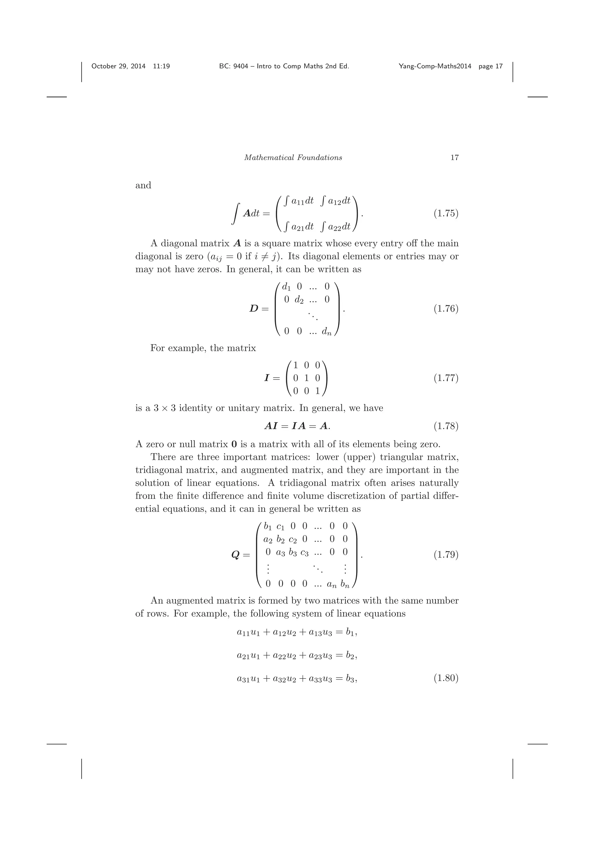
November 3, 2014 11:34 BC: 9404 – Intro to Comp Maths 2nd Ed. Yang-Comp-Maths2014 page 18 18 Introduction to Computational Mathematics can be written in a compact form in terms of matrices ⎛ ⎝ a11 a12 a13 a21 a22 a23 a31 a32 a33 ⎞ ⎠ ⎛ ⎝ u1 u2 u3 ⎞ ⎠ = ⎛ ⎝ b1 b2 b3 ⎞ ⎠, (1.81) or Au = b. (1.82) This can in turn be written as the following augmented form [A|b] = ⎛ ⎝ a11 a12 a13 b1 a21 a22 a23 b2 a31 a32 a33 b3 ⎞ ⎠ . (1.83) The augmented form is widely used in Gauss-Jordan elimination and linear programming. A lower (upper) triangular matrix is a square matrix with all the elements above (below) the diagonal entries being zeros. In general, a lower triangular matrix can be written as L = ⎛ ⎜ ⎜ ⎜ ⎝ l11 0 ... 0 l21 l22 ... 0 ... ln1 ln2 ... lnn ⎞ ⎟ ⎟ ⎟ ⎠ , (1.84) while the upper triangular matrix can be written as U = ⎛ ⎜ ⎜ ⎜ ⎝ u11 u12 ... u1n 0 u22 ... u2n ... 0 0 ... unn ⎞ ⎟ ⎟ ⎟ ⎠ . (1.85) Any n × n square matrix A = [aij] can be decomposed or factorized as a product of an L and a U, that is A = LU, (1.86) though some decomposition is not unique because we have n2 +n unknowns: n(n + 1)/2 coefficients lij and n(n + 1)/2 coefficients uij, but we can only provide n2 equations from the coefficients aij. Thus, there are n free parameters. The uniqueness of decomposition is often achieved by imposing either lii = 1 or uii = 1 where i = 1, 2, ..., n. Other LU variants include the LDU and LUP decompositions. An LDU decomposition can be written as A = LDU, (1.87)

October 29, 2014 11:19 BC: 9404 – Intro to Comp Maths 2nd Ed. Yang-Comp-Maths2014 page 19 Mathematical Foundations 19 where L and U are lower and upper matrices with all the diagonal entries being unity, and D is a diagonal matrix. On the other hand, the LUP decomposition can be expressed as A = LUP , or A = P LU, (1.88) where P is a permutation matrix which is a square matrix and has exactly one entry 1 in each column and each row with 0’s elsewhere. However, most numerical libraries and software packages use the following LUP decomposition P A = LU, (1.89) which makes it easier to decompose some matrices. However, the requirement for LU decompositions is relatively strict. An invertible matrix A has an LU decomposition provided that the determinants of all its diagonal minors or leading submatrices are not zeros. A simpler way of decomposing a square matrix A for solving a system of linear equations is to write A = D + L + U, (1.90) where D is a diagonal matrix. L and U are the strictly lower and upper triangular matrices without diagonal elements, respectively. This decomposition is much simpler to implement than the LU decomposition because there is no multiplication involved here. Example 1.4: The following 3 × 3 matrix A = ⎛ ⎝ 2 1 5 4 −4 5 5 2 −5 ⎞ ⎠, can be decomposed as A = LU. That is A = ⎛ ⎝ 1 0 0 l21 1 0 l31 l32 0 ⎞ ⎠ ⎛ ⎝ u11 u12 u13 0 u22 u23 0 0 u33 ⎞ ⎠, which becomes A = ⎛ ⎝ u11 u12 u13 l21u11 l21u12 + u22 l21u13 + u23 l31u11 l31u12 + l32u22 l31u13 + l32u23 + u33 ⎞ ⎠ = ⎛ ⎝ 2 1 5 4 −4 5 5 2 −5 ⎞ ⎠.

October 29, 2014 11:19 BC: 9404 – Intro to Comp Maths 2nd Ed. Yang-Comp-Maths2014 page 20 20 Introduction to Computational Mathematics This leads to u11 = 2, u12 = 1 and u13 = 5. As l21u11 = 4, so l21 = 4/u11 = 2. Similarly, l31 = 2.5. From l21u12 + u22 = −4, we have u22 = −4 − 2 × 1 = −6. From l21u13 + u23 = 5, we have u23 = 5 − 2 × 5 = −5. Using l31u12 +l32u22 = 2, or 2.5×1+l32 ×(−6) = 2, we get l32 = 1/12. Finally, l31u13 +l32u23 +u33 = −5 gives u33 = −5−2.5×5−1/12×(−5) = −205/12. Therefore, we now have ⎛ ⎝ 2 1 5 4 −4 5 5 2 −5 ⎞ ⎠ = ⎛ ⎝ 1 0 0 2 1 0 5/2 1/12 1 ⎞ ⎠ ⎛ ⎝ 2 1 5 0 −6 −5 0 0 −205/12 ⎞ ⎠. The L+D+U decomposition can be written as A = D + L + U = ⎛ ⎝ 2 0 0 0 −4 0 0 0 −5 ⎞ ⎠ + ⎛ ⎝ 0 0 0 4 0 0 5 2 0 ⎞ ⎠ + ⎛ ⎝ 0 1 5 0 0 5 0 0 0 ⎞ ⎠. 1.6 Determinant and Inverse The determinant of a square matrix A is a number or scalar obtained by the following recursive formula, or the cofactors, or the Laplace expansion by column or row. For example, expanding by row k, we have det(A) = |A| = n j=1 (−1)k+j akjMkj, (1.91) where Mij is the determinant of a minor matrix of A by deleting row i and column j. For a simple 2 × 2 matrix, its determinant simply becomes a11 a12 a21 a22 = a11a22 − a12a21. (1.92) The determinants of matrices have the following properties: |αA| = α|A|, |AT | = |A|, |AB| = |A||B|, (1.93) where A and B have the same size (n × n). An n × n square matrix is singular if |A| = 0, and is nonsingular if and only if |A| = 0. The trace of a square matrix tr(A) is deﬁned as the sum of the diagonal elements, tr(A) = n i=1 aii = a11 + a22 + ... + ann. (1.94)

October 29, 2014 11:19 BC: 9404 – Intro to Comp Maths 2nd Ed. Yang-Comp-Maths2014 page 21 Mathematical Foundations 21 The rank of a matrix A is the number of linearly independent vectors forming the matrix. Generally speaking, the rank of A satisfies rank(A) ≤ min(m, n). (1.95) For an n × n square matrix A, it is nonsingular if rank(A) = n. The inverse matrix A−1 of a square matrix A is defined as A−1 A = AA−1 = I. (1.96) More generally, A−1 l A = AA−1 r = I, (1.97) where A−1 l is the left inverse while A−1 r is the right inverse. If A−1 l = A−1 r , we say that the matrix A is invertible and its inverse is simply denoted by A−1 . It is worth noting that the unit matrix I has the same size as A. The inverse of a square matrix exists if and only if A is nonsingular or det(A) = 0. From the basic definitions, it is straightforward to prove that the inverse of a matrix has the following properties (A−1 )−1 = A, (AT )−1 = (A−1 )T , (1.98) and (AB)−1 = B−1 A−1 . (1.99) The inverse of a lower (upper) triangular matrix is also a lower (upper) triangular matrix. The inverse of a diagonal matrix D = ⎛ ⎜ ⎜ ⎜ ⎝ d1 0 ... 0 0 d2 ... 0 ... 0 0 ... dn ⎞ ⎟ ⎟ ⎟ ⎠ , (1.100) can simply be written as D−1 = ⎛ ⎜ ⎜ ⎜ ⎝ 1/d1 0 ... 0 0 1/d2 ... 0 ... 0 0 ... 1/dn ⎞ ⎟ ⎟ ⎟ ⎠ , (1.101) where di = 0. If any of these elements di is zero, then the diagonal matrix is not invertible as it becomes singular. For a 2 × 2 matrix, its inverse is simply A = a b c d , A−1 = 1 ad − bc d −b −c a . (1.102)

October 29, 2014 11:19 BC: 9404 – Intro to Comp Maths 2nd Ed. Yang-Comp-Maths2014 page 22 22 Introduction to Computational Mathematics Example 1.5: For two matrices, A = ⎛ ⎝ 4 5 0 −2 2 5 2 −3 1 ⎞ ⎠, B = ⎛ ⎝ 2 3 0 −2 5 2 ⎞ ⎠, their transpose matrices are AT = ⎛ ⎝ 4 −2 2 5 2 −3 0 5 1 ⎞ ⎠, BT = 2 0 5 3 −2 2 . Let D = AB be their product; we have AB = D = ⎛ ⎝ D11 D12 D21 D22 D31 D32 ⎞ ⎠. The ﬁrst two entries are D11 = 3 j=1 A1jBj1 = 2 × 4 + 5 × 0 + 0 × 5 = 8, and D12 = 3 j=1 A1jBj2 = 4 × 3 + 5 × (−2) + 0 × 2 = 2. Similarly, the other entries are: D21 = 21, D22 = 0, D31 = 9, D33 = 14. Therefore, we get AB = ⎛ ⎝ 4 5 0 −2 2 5 2 −3 1 ⎞ ⎠ ⎛ ⎝ 2 3 0 −2 5 2 ⎞ ⎠ = D = ⎛ ⎝ 8 2 21 0 9 14 ⎞ ⎠. However, the product BA does not exist, though BT AT = 8 21 9 2 0 14 = DT = (AB)T . The inverse of A is A−1 = 1 128 ⎛ ⎝ 17 −5 25 12 4 −20 2 22 18 ⎞ ⎠,

October 29, 2014 11:19 BC: 9404 – Intro to Comp Maths 2nd Ed. Yang-Comp-Maths2014 page 23 Mathematical Foundations 23 and the determinant of A is det(A) = 128. It is straightforward to verify that AA−1 = A−1 A = I = ⎛ ⎝ 1 0 0 0 1 0 0 0 1 ⎞ ⎠. For example, the first entry is obtained by 3 j=1 A1jA−1 j1 = 4 × 17 128 + 5 × 12 128 + 0 × 2 128 = 1. Other entries can be verified similarly. Finally, the trace of A is tr(A) = A11 + A22 + A33 = 4 + 2 + 1 = 7. The algorithmic complexity of most algorithms for obtaining the inverse of a general square matrix is O(n3 ). That is why most modern algorithms try to avoid the direct inverse of a large matrix. Solution of a large matrix system is instead carried out either by partial inverse via decomposition or by iteration (or a combination of these two methods). If the matrix can be decomposed into triangular matrices either by LU factorization or direction decomposition, the aim is then to invert a triangular matrix, which is simpler and more efficient. For a triangular matrix, the inverse can be obtained using algorithms of O(n2 ) complexity. Similarly, the solution of a linear system with a lower (upper) triangular matrix A can be obtained by forward (back) substitutions. In general, for a lower triangular matrix A = ⎛ ⎜ ⎜ ⎜ ⎝ α11 0 ... 0 α12 α22 ... 0 ... αn1 αn2 ... αnn ⎞ ⎟ ⎟ ⎟ ⎠ , (1.103) the forward substitutions for the system Au = b can be carried out as follows: u1 = b1 α11 , u2 = 1 α22 (b2 − α21u1),

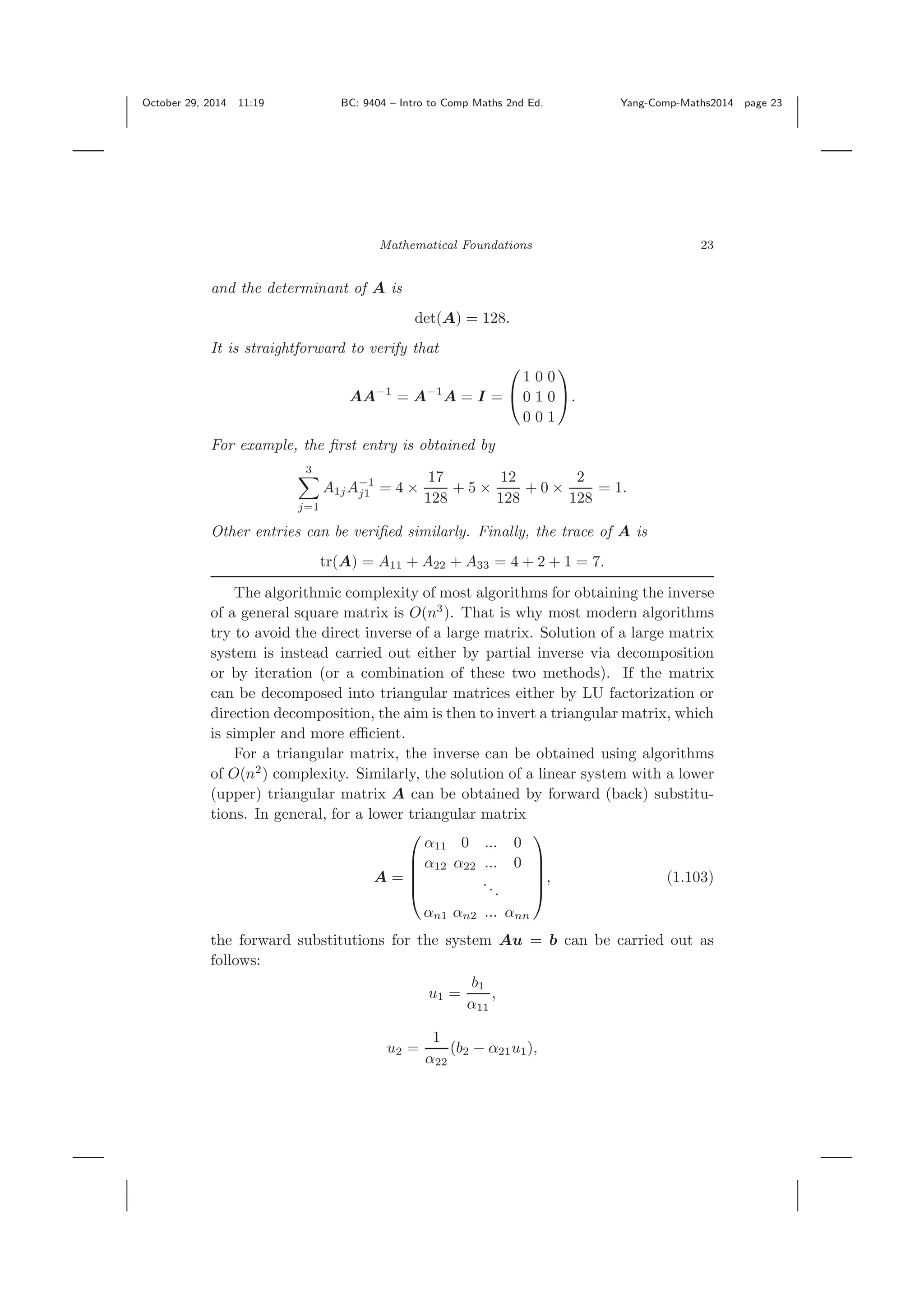
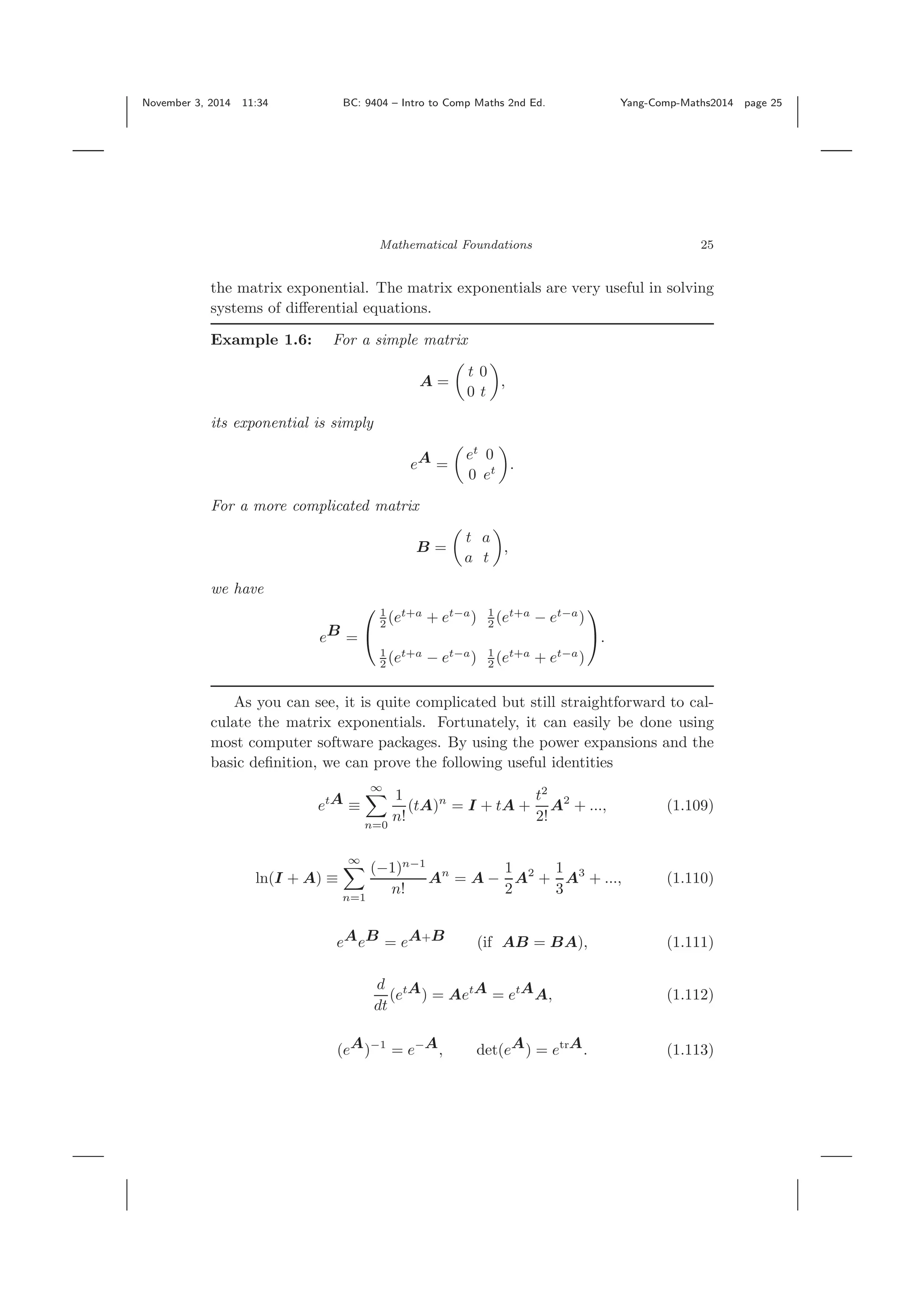
November 3, 2014 11:34 BC: 9404 – Intro to Comp Maths 2nd Ed. Yang-Comp-Maths2014 page 24 24 Introduction to Computational Mathematics ui = 1 αii (bi − i−1 j=1 αijuj), (1.104) where i = 2, ..., n. We see that it takes 1 division to get u1, 3 floating point calculations to get u2, and (2i− 1) to get ui. So the total algorithmic complexity is O(1 + 3 + ... + (2n − 1)) = O(n2 ). Similar arguments apply to the upper triangular systems. The inverse A−1 of a lower triangular matrix can in general be written as A−1 = ⎛ ⎜ ⎜ ⎜ ⎝ β11 0 ... 0 β21 β22 ... 0 ... βn1 βn2 ... βnn ⎞ ⎟ ⎟ ⎟ ⎠ = B = B1 B2 ... Bn , (1.105) where Bj are the j-th column vector of B. The inverse must satisfy AA−1 = I or A B1 B2 ... Bn = I = e1 e2 ... en , (1.106) where ej is the j-th unit vector of size n with the j-th element being 1 and all other elements being zero. That is eT j = 0 0 ... 1 0 ... 0 . In order to obtain B, we have to solve n linear systems AB1 = e1, AB2 = e2, ..., ABn = en. (1.107) As A is a lower triangular matrix, the solution of ABj = ej can easily be obtained by direct forward substitutions discussed earlier in this section. 1.7 Matrix Exponential Sometimes, we need to calculate exp[A], where A is a square matrix. In this case, we have to deal with matrix exponentials. The exponential of a square matrix A is defined as eA ≡ ∞ n=0 1 n! An = I + A + 1 2! A2 + ..., (1.108) where I is an identity matrix with the same size as A, and A2 = AA and so on. This (rather odd) definition in fact provides a method of calculating

November 3, 2014 11:34 BC: 9404 – Intro to Comp Maths 2nd Ed. Yang-Comp-Maths2014 page 25 Mathematical Foundations 25 the matrix exponential. The matrix exponentials are very useful in solving systems of diﬀerential equations. Example 1.6: For a simple matrix A = t 0 0 t , its exponential is simply eA = et 0 0 et . For a more complicated matrix B = t a a t , we have eB = ⎛ ⎝ 1 2 (et+a + et−a ) 1 2 (et+a − et−a ) 1 2 (et+a − et−a ) 1 2 (et+a + et−a ) ⎞ ⎠. As you can see, it is quite complicated but still straightforward to calculate the matrix exponentials. Fortunately, it can easily be done using most computer software packages. By using the power expansions and the basic deﬁnition, we can prove the following useful identities etA ≡ ∞ n=0 1 n! (tA)n = I + tA + t2 2! A2 + ..., (1.109) ln(I + A) ≡ ∞ n=1 (−1)n−1 n! An = A − 1 2 A2 + 1 3 A3 + ..., (1.110) eAeB = eA+B (if AB = BA), (1.111) d dt (etA) = AetA = etAA, (1.112) (eA)−1 = e−A, det(eA) = etrA. (1.113)

October 29, 2014 11:19 BC: 9404 – Intro to Comp Maths 2nd Ed. Yang-Comp-Maths2014 page 26 26 Introduction to Computational Mathematics 1.8 Hermitian and Quadratic Forms The matrices we have discussed so far are real matrices because all their elements are real. In general, the entries or elements of a matrix can be complex numbers, and the matrix becomes a complex matrix. For a matrix A, its complex conjugate A∗ is obtained by taking the complex conjugate of each of its elements. The Hermitian conjugate A† is obtained by taking the transpose of its complex conjugate matrix. That is to say, for A = ⎛ ⎝ a11 a12 ... a21 a21 ... ... ... ... ⎞ ⎠, (1.114) we have A∗ = ⎛ ⎝ a∗ 11 a∗ 12 ... a∗ 21 a∗ 22 ... ... ... ... ⎞ ⎠, (1.115) and A† = (A∗ )T = (AT )∗ = ⎛ ⎝ a∗ 11 a∗ 21 ... a∗ 12 a22 ... ... ... ... ⎞ ⎠. (1.116) A square matrix A is called orthogonal if and only if A−1 = AT . If a square matrix A satisﬁes A∗ = A, it is called an Hermitian matrix. It is an anti-Hermitian matrix if A∗ = −A. If the Hermitian matrix of a square matrix A is equal to the inverse of the matrix (or A† = A−1 ), it is called a unitary matrix. Example 1.7: For a complex matrix A = 2 + 3iπ 1 + 9i 0 eiπ −2i i sin θ , its complex conjugate A∗ is A∗ = 2 − 3iπ 1 − 9i 0 e−iπ 2i −i sin θ . The Hermitian conjugate of A is A† = ⎛ ⎝ 2 − 3iπ e−iπ 1 − 9i 2i 0 −i sinθ ⎞ ⎠ = (A∗ )T .

October 29, 2014 11:19 BC: 9404 – Intro to Comp Maths 2nd Ed. Yang-Comp-Maths2014 page 27 Mathematical Foundations 27 For the rotation matrix A = cos θ sin θ − sin θ cos θ , its inverse and transpose are A−1 = 1 cos2 θ + sin2 θ cos θ − sin θ sin θ cos θ , and AT = cos θ − sin θ sin θ cos θ . Since cos2 θ + sin2 θ = 1, we have AT = A−1 . Therefore, the original rotation matrix A is orthogonal. A very useful concept in computational mathematics and computing is quadratic forms. For a real vector qT = (q1, q2, q3, ..., qn) and a real symmetric square matrix A, a quadratic form ψ(q) is a scalar function deﬁned by ψ(q) = qT Aq = q1 q2 ... qn ⎛ ⎜ ⎜ ⎝ A11 A12 ... A1n A21 A22 ... A2n ... ... ... ... An1 An2 ... Ann ⎞ ⎟ ⎟ ⎠ ⎛ ⎜ ⎜ ⎜ ⎝ q1 q2 ... qn ⎞ ⎟ ⎟ ⎟ ⎠ , (1.117) which can be written as ψ(q) = n i=1 n j=1 qiAijqj. (1.118) Since ψ is a scalar, it should be independent of the coordinates. In the case of a square matrix A, ψ might be more easily evaluated in certain intrinsic coordinates Q1, Q2, ..., Qn. An important result concerning the quadratic form is that it can always be written through appropriate transformations as ψ(q) = n i=1 λiQ2 i = λ1Q2 1 + λ2Q2 2 + ... + λnQ2 n, (1.119) where λi are the eigenvalues of the matrix A determined by det |A − λI| = 0, (1.120) and Qi are the intrinsic components along directions of the eigenvectors in this case.

October 29, 2014 11:19 BC: 9404 – Intro to Comp Maths 2nd Ed. Yang-Comp-Maths2014 page 28 28 Introduction to Computational Mathematics The natural extension of quadratic forms is the Hermitian form which is the quadratic form for a complex Hermitian matrix A. Furthermore, the matrix A can consist of linear operators and functionals in addition to numbers. Example 1.8: For a vector q = (q1, q2) and the square matrix A = 2 −5 −5 2 , we have a quadratic form ψ(q) = q1 q2 2 −5 −5 2 q1 q2 = 2q2 1 − 10q1q2 + 2q2 2. The eigenvalues of the matrix A is determined by 2 − λ −5 −5 2 − λ = 0, whose solutions are λ1 = 7 and λ2 = −3 (see the next section for further details). Their corresponding eigenvectors are v1 = − √ 2/2√ 2/2 , v2 = √ 2/2√ 2/2 . We can see that v1 ·v2 = 0, which means that these two eigenvectors are orthogonal. Writing the quadratic form in terms of the intrinsic coordinates, we have ψ(q) = 7Q2 1 − 3Q2 2. Furthermore, if we assume ψ(q) = 1 as a simple constraint, then the equation 7Q2 1 − 3Q2 2 = 1 corresponds to a hyperbola. 1.9 Eigenvalues and Eigenvectors The eigenvalue λ of any n × n square matrix A is determined by Au = λu, (1.121) or (A − λI)u = 0, (1.122) where I is a unitary matrix with the same size as A. Any non-trivial solution requires that det |A − λI| = 0, (1.123)

November 3, 2014 11:34 BC: 9404 – Intro to Comp Maths 2nd Ed. Yang-Comp-Maths2014 page 29 Mathematical Foundations 29 or a11 − λ a12 ... a1n a21 a22 − λ ... a2n ... ... an1 an2 ... ann − λ = 0, (1.124) which again can be written as a polynomial λn + αn−1λn−1 + ... + α0 = (λ − λ1)...(λ − λn) = 0, (1.125) where λis are the eigenvalues which could be complex numbers. In general, the determinant is zero, which leads to a polynomial of order n in λ. For each eigenvalue λ, there is a corresponding eigenvector u whose direction can be uniquely determined. However, the length of the eigenvector is not unique because any non-zero multiple of u will also satisfy equation (1.121), and thus can be considered as an eigenvector. For this reason, it is usually necessary to apply additional conditions by setting the length as unity, and subsequently the eigenvector becomes a unit eigenvector. Generally speaking, a real n × n matrix A has n eigenvalues λi(i = 1, 2, ..., n), however, these eigenvalues are not necessarily distinct. If the real matrix is symmetric, that is to say AT = A, then the matrix has n distinct eigenvectors, and all the eigenvalues are real numbers. The eigenvalues λi are related to the trace and determinant of the matrix tr(A) = n i=1 aii = λ1 + λ2 + ... + λn = n i=1 λi, (1.126) and det(A) = |A| = n i=1 λi. (1.127) Example 1.9: The eigenvalues of the square matrix A = 4 9 2 −3 , can be obtained by solving 4 − λ 9 2 −3 − λ = 0. We have (4 − λ)(−3 − λ) − 18 = (λ − 6)(λ + 5) = 0.

October 29, 2014 11:19 BC: 9404 – Intro to Comp Maths 2nd Ed. Yang-Comp-Maths2014 page 30 30 Introduction to Computational Mathematics Thus, the eigenvalues are λ = 6 and λ = −5. Let v = (v1 v2)T be the eigenvector; we have for λ = 6 |A − λI| = −2 9 2 −9 v1 v2 = 0, which means that −2v1 + 9v2 = 0, 2v1 − 9v2 = 0. These two equations are virtually the same (not linearly independent), so the solution is v1 = 9 2 v2. Any vector parallel to v is also an eigenvector. In order to get a unique eigenvector, we have to impose an extra requirement, that is, the length of the vector is unity. We now have v2 1 + v2 2 = 1, or ( 9v2 2 )2 + v2 2 = 1, which gives v2 = ±2/ √ 85, and v1 = ±9/ √ 85. As these two vectors are in opposite directions, we can choose any of the two directions. So the eigenvector for the eigenvalue λ = 6 is v = ⎛ ⎝ 9/ √ 85 2/ √ 85 ⎞ ⎠. Similarly, the corresponding eigenvector for the eigenvalue λ = −5 is v = (− √ 2/2 √ 2/2)T . Furthermore, the trace and determinant of A are tr(A) = 4 + (−3) = 1, det(A) = 4 × (−3) − 2 × 9 = −30. The sum of the eigenvalues is 2 i=1 λi = 6 + (−5) = 1 = tr(A), while the product of the eigenvalues is 2 i=1 λi = 6 × (−5) = −30 = det(A). For any real square matrix A with the eigenvalues λi = eig(A), the eigenvalues of αA are αλi where α = 0 ∈ . This property becomes handy when rescaling the matrices in some iteration formulae so that the rescaled scheme becomes more stable. This is also the major reason why the pivoting and removing/rescaling of exceptionally large elements works.

October 29, 2014 11:19 BC: 9404 – Intro to Comp Maths 2nd Ed. Yang-Comp-Maths2014 page 31 Mathematical Foundations 31 1.10 Definiteness of Matrices A square symmetric matrix A is said to be positive definite if all its eigenvalues are strictly positive (λi > 0 where i = 1, 2, ..., n). By multiplying (1.121) by uT , we have uT Au = uT λu = λuT u, (1.128) which leads to λ = uT Au uT u . (1.129) This means that uT Au > 0, if λ > 0. (1.130) In fact, for any vector v, the following relationship holds vT Av > 0. (1.131) Since v can be a unit vector, thus all the diagonal elements of A should be strictly positive as well. If all the eigenvalues are non-negative or λi ≥ 0, then the matrix is called positive semi-definite. In general, an indefinite matrix can have both positive and negative eigenvalues. The inverse of a positive definite matrix is also positive definite. For a linear system Au = f where f is a known column vector, if A is positive definite, then the system can be solved more efficiently by matrix decomposition methods. Example 1.10: In general, a 2 × 2 symmetric matrix A A = α β β γ , is positive definite if αu2 1 + 2βu1u2 + γu2 2 > 0, for all u = (u1, u2)T = 0. The inverse of A is A−1 = 1 αγ − β2 γ −β −β α , which is also positive definite. As the eigenvalues of A = 1 2 2 1 ,

October 29, 2014 11:19 BC: 9404 – Intro to Comp Maths 2nd Ed. Yang-Comp-Maths2014 page 32 32 Introduction to Computational Mathematics are λ = 3, −1, the matrix is indefinite. For another matrix B = 4 6 6 20 , we can find its eigenvalues using a similar method as discussed earlier, and the eigenvalues are λ = 2, 22. So matrix B is positive definite. The inverse of B B−1 = 1 44 20 −6 −6 4 , is also positive definite because B−1 has two eigenvalues: λ = 1/2, 1/22. We have briefly reviewed the basic algebra of vectors and matrices as well as some basic calculus, now can move onto more algorithm-related topics such as algorithm complexity.

October 29, 2014 11:19 BC: 9404 – Intro to Comp Maths 2nd Ed. Yang-Comp-Maths2014 page 33 Chapter 2 Algorithmic Complexity, Norms and Convexity When analyzing an algorithm, we often discuss its computational complexity. This also allows us to compare one algorithm with other algorithms in terms of various performance measures. 2.1 Computational Complexity The efficiency of an algorithm is often measured by its algorithmic complexity or computational complexity. In the literature, this complexity is also called Kolmogorov complexity. For a given problem size n, the complexity is denoted using Big-O notations such as O(n2 ) or O(n log n). For the sorting algorithm for a given number of n data entries, sorting these numbers into either ascending or descending order will take the computational time as a function of the problem size n. O(n) means a linear complexity, while O(n2 ) has a quadratic complexity. That is, if n is doubled, then the computational time or computational efforts will double for linear complexity, but it will quadruple for quadratic complexity. For example, the bubble sorting algorithm starts at the beginning of the data set by comparing the first two elements. If the first is smaller than the second, then swap them. This comparison and swap process continues for each possible pair of adjacent elements. There are n × n pairs as we need two loops over the whole data set, then the algorithm complexity is O(n2 ). On the other hand, the quicksort algorithm uses a divide-and-conquer approach via partition. By first choosing a pivot element, we then put all the elements into two sublists with all the smaller elements before the pivot and all the greater elements after it. Then, the sublists are recursively sorted in a similar manner. This algorithm will result in a complexity of O(n log n). The quicksort is much more efficient than the bubble algorithm. 33

Introduction to Computational Mathematics (2nd Edition, 2015)

More Related Content

Similar to Introduction to Computational Mathematics (2nd Edition, 2015)

More from Xin-She Yang

Recently uploaded

Introduction to Computational Mathematics (2nd Edition, 2015)